Image Compression Using Cascaded Neural Networks

(1)

ScholarWorks@UNO

University of New Orleans Theses and

Dissertations Dissertations and Theses

8-7-2003

Image Compression Using Cascaded Neural Networks

Chigozie Obiegbu

University of New Orleans

Follow this and additional works at: https://scholarworks.uno.edu/td

Recommended Citation Recommended Citation

Obiegbu, Chigozie, "Image Compression Using Cascaded Neural Networks" (2003). University of New Orleans Theses and Dissertations. 34.

https://scholarworks.uno.edu/td/34

This Thesis is protected by copyright and/or related rights. It has been brought to you by ScholarWorks@UNO with permission from the rights-holder(s). You are free to use this Thesis in any way that is permitted by the copyright and related rights legislation that applies to your use. For other uses you need to obtain permission from the rights-holder(s) directly, unless additional rights are indicated by a Creative Commons license in the record and/or on the work itself.

(2)

CASCADED NEURAL NETWORKS

A Thesis

Submitted to the Graduate Faculty of the University of New Orleans

in partial fulfillment of the requirements for the degree of

Master of Science in

The Department of Electrical Engineering

by

Chigozie Obiegbu

(3)

ii

ACKNOWLEDGMENTS

The completion of this thesis has involved an enormous amount of help from a number of people. First and foremost of these is Dr. Dimitrios Charalampidis, my thesis advisor, for providing the original ideas, suggestions, and motivation for the work. He freely bestowed his time, guidance, brilliance, and wisdom considerably beyond the call of duty; and was a model of professorial responsibility, professionalism, and commitment. What I have learned from him cannot be quantified. Special thanks to other members of my thesis committee, Dr. Juliette Ioup and Dr. Terry Riemer for enriching my experience in academia by sharing with me their intellectual curiosity, professional insight and integrity, and personal warmth and understanding through their courses. I would especially like to thank Dr. Juliette Ioup for carefully reading through the entire draft of my thesis and offering several helpful editorial comments.

(4)

iii

LIST OF TABLES

(7)

vi

LIST OF FIGURES

1.0 Block diagram of JPEG compression ...10

2.0 Zigzag sequence for Binary Encoding ...12

3.1 Graph of hyperbolic tangent function...21

3.2 Multiple- input neuron...22

3.3 Architecture of Backpropagation Neural Network ...30

3.4 Architecture of RBF ...41

3.5 Architecture of GRNN...47

3.6 Architecture of Modular Neural Network...52

3.7 Architecture of Probabilistic Neural Network ...57

3.8 Cascade Correlation Network ...68

4.0 Image Compression Block Diagram...73

4.1 Single-structure neural network image compression/decompression scheme ...76

4.2 (a) Encoding scheme for proposed cascade architecture ...82

4.2 (b) Decoding scheme for proposed cascade architecture...82

5.1 PSNR vs. CR for reconstructed Lena image ...85

5.2 PSNR vs. CR for reconstructed Peppers image ...86

5.3 PSNR vs. CR for reconstructed Baboon image ...87

5.4 (a) Original Lena image ...88

5.4 (b) Reconstructed Lena image at 8:1 CR using single-structure NN...88

(8)

vii

(9)

viii

ABSTRACT

(10)

CHAPTER 1 Introduction

Computer images are extremely data intensive and hence require large amounts of memory for storage. As a result, the transmission of still images from one machine to another can be very time consuming. For this reason still image compression is subject of an intense worldwide research effort [1]-[8]. By using data compression techniques, it is possible to remove some of the redundant information contained in images, requiring less storage space and less time to transmit. The objective of digital image compression techniques is the minimization of the number of bits required to represent an image, while maintaining an acceptable image quality. Another issue in image compression and decompression is the processing speed, especially in real-time applications. It is often desirable to be able to carry out compression and decompression in real-time without reducing image quality.

(11)

the transmission of a compressed picture over a mobile or cordless telephone. In these applications, the bit error rates due to noise on the transmission channel may be as high as 10−2[12], [14]. At these error rates, JPEG and similar compression algorithms, which rely on entropy coding, are not suitable [12].

Recently, neural networks have proved to be useful in image compression because of their parallel architecture and flexibility [15]-[20]. They do not use entropy coding and are therefore intrinsically robust, making them an attractive choice for high noise environments. Of course a price must be paid for this robustness. In this case, the price is a reduction in decompressed image quality for the same compression efficiency. However, as shall be seen in chapter 4, the reduction in image quality is not excessive.

Although the parallel-structure neural networks are robust, they suffer from several drawbacks. The main drawbacks are:

1) high computational complexity;

2) moderate reconstructed picture quality; 3) variable bit-rate;

(12)

The chapters of this thesis are organized as follows: Chapter 2 briefly reviews three of the major approaches to image compression, namely predictive coding, transform coding and vector quantization. In particular, the JPEG technique is described. Chapter 3 discusses NN technology, including various architectures and algorithms. These architectures include Backpropagation, Radial-basis function, General Regression, Modular, Probabilistic, and Learning Vector Quantization. The single-structure NN consisting of two layers and the parallel-structure NN are embedded in the discussion. In Chapter 4, the single-structure NN as an image compression tool is implemented, and the proposed NN method using a cascade of feedforward networks is presented. A background on this approach is given followed by its application to image compression. Chapter 5 presents experimental results. The error metrics used in computing the results are described. Graphical and pictorial results are fully illustrated. Performance comparisons are made with JPEG and single-structure/parallel-structure NNs. Issues relating to a comprehensive evaluation of the image compression techniques presented herein are discussed in Chapter 6. The practicality and usefulness of the new method is mentioned.

(13)

CHAPTER 2 Techniques for Image Compression

Image compression methods are categorized as lossless and lossy. Lossless methods preserve all original information without changing it. Lossy methods reduce information to attain better compression ratio. Lossless compression has been found to be adequate when low compression ratios are acceptable. Significantly substantial compression ratios can only be achieved with lossy compression schemes, which will be the main focus of this thesis. Due to the extensive breadth of this field, it is impossible to list all of the currently available image compression techniques. However, existing research fall into one of three major categories: vector quantization, predictive coding, or transform coding.

2.1 Vector Quantization

(14)

Vector Quantization (VQ) [9] – [11] uses a codebook containing pixel patterns with corresponding index for each of them. The main idea of VQ in image coding is then to represent arrays of pixels by an index in the codebook. In this way, compression is achieved since the size of the index is usually a small fraction of that of the block of pixels. The codebook is used to quantize the incoming vectors and is analogous to the quantization levels in a scalar quantizer. A good codebook can reduce the overall distortion of the reconstructed image, and is determinative to the performance of the VQ process.

At the encoder, the incoming image is partitioned into blocks of sub-images. These blocks have the dimension equal to entries in codebook, so comparison can be done easily between them. An input vector Xn consisting of blocks of pixels is quantized.

This is done by encoding Xn into a binary index in which points to an entry in the

codebook. This in then serves as an index for the output reproduction vector or codeword.

The standard approach to calculate the codebook is by way of the Linde, Buzo, and Gray (LBG) algorithm [9]. Finally, the concatenation of all in represents the compressed image.

However, the choice of index in will be different when using different mapping rules.

These mapping rules often depend on minimizing a predefined distortion measure

d(Xn,Yin), where Xn and Yin are the vectors from the image and from the codebook

(15)

The main advantages of VQ are the simplicity of its idea and the possible efficient implementation of the decoder. Moreover, VQ is theoretically an efficient method for image compression, and superior performance will be gained for large vectors. However, in order to use large vectors, VQ encoding becomes complex, which requires many computational resources (e.g., memory, computations per pixel) in order to efficiently construct and search a codebook. For instance, while the LGB algorithm converges to a local minimum, it is not guaranteed to reach the global minimum. In addition, the algorithm is very sensitive to the initial codebook. Furthermore, the algorithm is slow since it requires, on each iteration, an exhaustive search through the entire codebook. More research on reducing this complexity must be done in order to make VQ a practical image compression method with superior quality.

2.2 Predictive Coding

Predictive image coding algorithms [5] are used primarily to exploit correlation between adjacent pixels. They predict the value of a given pixel based on the values of the surrounding pixels. Due to the correlation property among adjacent pixels in an image, the use of predictor can reduce the amount of information bits required to represent the image. This can accomplished through the use of predictive coding or differential pulse-code modulation (DPCM).

(16)

the difference decreases, resulting in higher predictive gain and therefore a higher compression ratio.

The problem of course is how to design the predictor. One approach is to use a statistical model of the data to derive a function which relates the values of the neighboring pixels to that of the current one in an optimal manner. An autoregressive model (AR) is one such model which has been successfully applied to images. For a

pthorder causal AR process, the nth value x(n) is related to the previous pvalues in the following manner:

n p

j

jx n j

n

x =

∑

ω − +ε

= ) ( ) ( 1

, (2.1)

where {ω_j} is a set of AR coefficients, and {εn} is a set of zero-mean independent and

identically distributed random variables. In this case, the predicted value is a linear sum of neighboring samples (pixels) as shown by

) ( ) ( ˆ 1 j n x n x p j j − =

∑

=

ω . (2.2)

Equation (2.2) is the basis of linear predictive coding. To minimize the mean squared error E[(xˆ−x)2], the following relationship must be satisfied:

,

d

Rw= (2.3)

where [R]ij = E[x(i)x(j)] is ijthelement of the autocovariance matrix R and

)] ( ) ( ˆ [x n x j E

(17)

2.3 Transform Coding

Another approach to image compression is the use of transformations that operate on an image to produce a set of coefficients [5]. A subset of these coefficients is chosen and quantized for transmission across a channel or for storage. The goal of this technique is to choose a transformation for which such a subset of coefficients is adequate to reconstruct an image with minimum discernible distortion.

A simple and powerful class of transform coding techniques is linear block transform coding. An image is subdivided into non-overlapping blocks of n×n pixels which can be considered as N-dimensional vectors x with N =n×n. A linear transformation, which can be written as an M ×N-dimensional matrix W with M ≤N, is performed on each block, with the Mrows of W, wi being the basis vectors of the

transformation. The resulting M-dimensional coefficient vector y is calculated as

.

Wx

y= (2.4)

If the basis vectors wi are orthogonal, that is,

  

≠ = =

j i

j i w

wT _j i

, 0

, 1

, (2.5)

then the inverse transformation is given by the transpose of the forward transformation matrix resulting in the reconstructed vector:

y W

xˆ= T . (2.6)

(18)

] [xxT E

=

Σ . (2.7)

The KLT also produces uncorrelated coefficients and therefore results in the most efficient coding of the data since the redundancy due to the high degree of correlation between neighboring pixels is removed. The KLT is related to principal component analysis (PCA) [23], since the basis vectors are also the M principal components of the data. Because the KLT is an orthogonal transformation, its inverse is simply its transpose.

A number of practical difficulties exist when trying to implement the above approach. The calculation of the estimate of the covariance of an image may be unwieldy and may require a large amount of memory. In addition, the solution for the eigenvectors and eigenvalues is computationally intensive. Finally, the calculation of the forward and inverse transforms is of order O(MN) for each image block. Due to these difficulties, fixed-basis transforms such as the discrete cosine transform (DCT) [22], which can be computed in order, O(NlogN), are typically used when implementing block transform schemes.

2.3.1 Discrete Cosine Transform

(19)

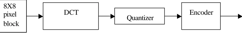
Figure 1 describes the baseline JPEG process. The compression scheme is divided into the following stages:

1. Apply a DCT to blocks of pixels, thus removing redundant image data.

2. Quantize each block of DCT coefficients using weighting functions optimized for the human eye.

3. Encode the resulting coefficients (image data) using a Huffman variable word-length algorithm to remove redundancies in the coefficients.

The image is first subdivided into 8 x 8 blocks of pixels. As each 8 x 8 block or sub-image is encountered, its 64 pixels are level shifted by subtracting the quantity 2n−1, where 2 is the maximum number of gray levels. n

Figure 1.0: Block diagram of JPEG compression.

The 2-D discrete cosine transform of the block is then computed. The DCT helps separate the image into parts (or spectral sub-bands) of differing importance with respect to the image's visual quality. The DCT is similar to the discrete Fourier transform: it transforms a signal or image from the spatial domain to the spatial frequency domain. With an input image, A, the output image, B is:

∑ ∑

− = − =      +       + = 1 0 2 1 0 1 1 2 ) 1 2 ( 2 cos ) 1 2 ( 2 cos ) , ( ) ( ) ( 4 1 ) , ( N i N j j N v i N u j i A v C u C v u

B π π . (2.8)

where C(u), C(v) = 1/√2 for u,v = 0 and 1 otherwise 8X8

pixel block

DCT

(20)

The input image is N₂ pixels wide by N₁ pixels high; A(i, j) is the intensity of the pixel in row i and column j. B(u,v)is the DCT coefficient in row u and column v of the DCT matrix. The DCT input is an 8 by 8 array of integers. This array contains each pixel's gray scale level; 8 bit pixels have levels from 0 to 255. The output array of DCT coefficients contains integers; these can range from -1024 to +1023. For most images, much of the signal energy lies at low frequencies; these appear in the upper left corner of the DCT. The lower right values represent higher frequencies, and are often small - small enough to be neglected with little visible distortion. A quantizer rounds off the DCT coefficients according to a quantization matrix. This matrix is the 8 by 8 matrix of step sizes (sometimes called quantums) - one element for each DCT coefficient. It is usually symmetric. Step sizes will be small in the upper left (low frequencies), and large in the lower right (high frequencies); a step size of 1 is the most precise. The quantizer divides the DCT coefficient by its corresponding quantum, and then rounds to the nearest integer. Large quantums drive small coefficients down to zero. The result: many high frequency coefficients become zero, and therefore easier to code. The low frequency coefficients undergo only minor adjustment. This step causes the lossy nature of JPEG, but allows for large compression ratios.

(21)

The number of previous zeros and the bits needed for the current number's amplitude form a pair. Each pair has its own code word, assigned through a variable length code (for example Huffman, Shannon-Fano or Arithmetic coding). JPEG outputs the code word of the pair, and then the codeword for the coefficient's amplitude (also from a variable length code). After each block, JPEG writes a unique end-of-block sequence to the output stream, and moves to the next block. When finished with all blocks, JPEG writes the end-of-file marker. At this point, the JPEG data stream is ready to be transmitted across a communications channel or encapsulated inside an image file format.

JPEG is not always an ideal compression solution. There are several reasons:

§ Does not fit every compression need. Images containing large areas of a single color do not compress very well.

(22)

§ Hard to implement.

§ Not supported by very many file formats.

Recently, novel approaches have been introduced based on pyramidal structures [24], wavelet transforms [25], and fractal transforms [26]. These and some other new techniques [27] inspired by the representation of visual information in the brain can achieve high compression ratios with good visual quality but are nevertheless computationally intensive.

(23)

CHAPTER 3 Artificial Neural Network Technology- an Overview

Artificial Neural networks are software or hardware systems that try to simulate the human brain functionality. From the beginning of their presence in science, Neural Networks (NNs) are being investigated with two different scientific approaches. First, the biological aspect explores NNs as simplified simulations of the human brain and uses them to test hypotheses about human brain functioning. The second approach treats NNs as technological systems for complex information processing. This thesis is focused on the second approach by which NNs are evaluated according to their efficiency to deal with complex problems, especially in the areas of association, classification and prediction, but specifically in the area of image processing.

(24)

efficiently than traditional modeling and statistical methods. It is mathematically proven (using the Ston-Weierstrass, Hahn-Banach and other theorems and corollaries [36]) that two-layer neural networks having arbitrarily squashing transfer functions are capable of approximating any nonlinear function.

3.1 Basic Principles of Learning in Neural Networks

(25)

ji

w denotes the connection weight from neuron j to neuron i (wij is the weight of the

reverse connection from neuron i to neuron j). If neuron i is connected to neurons called 1,2,...,n,their weights are stored in the variables w₁_i,w₂_i,w_ni. A neuron receives as many inputs as there are input connections to that neuron and produces a single output to other neurons according to a transfer function.

The process of neural network design consists of four phases: 1. arranging neurons in various layers,

2. determining the type of connections between neurons (inter-layer and intra-layer connections),

3. determining the way neuron receives input and produce output, and 4. determining the learning rule for adjusting the connection weights.

The result of NN design is the NN architecture. According to the above design processes, the criteria to distinguish NN architectures are as follows:

§ number of layers,

§ type of connection between neurons,

§ connection between input and output data,

§ input and transfer functions,

§ type of learning,

§ certainty of firing,

§ temporal characteristics, and

(26)

3.1.1 Type of Connection between Neurons

Connections in the network can be realized between two layers (inter-layer connections) and between neurons in one layer (intra-layer connections) [28]. Inter-layer connections can be classified as: fully connected - each neuron in the first layer is connected to each neuron in the second layer; partially connected - each neuron in the first layer should not necessarily be connected to every neuron in the second layer; feed-forward - connection between neurons is one-directional, neurons in the first layer send their output to the neurons in the second layer, but they do not receive any feedback; bi-directional - there is a feedback when the neurons from the second layer send their output back to the neurons in the first layer; hierarchical - neurons in one layer are connected only to the neurons of the next neighbor layer; resonance - two-directional connection where neurons continue to send information between layers until a certain condition is satisfied.

Examples of some well known NN architectures with inter-layer connections:

§ Perceptron (developed by Frank Rosenblat, 1957) - first NN, two-layered, fully connected,

§ ADALINE (developed by Bernard Widrow, Marcian E. Hoff, 1962) - two-layered, fully connected,

§ Backpropagation (developed by Paul Werbos, 1974, extended by Rumelhart, Hinton, Williams, 1986) - first NN with one or more hidden layers, connection between hidden layers is hierarchical,

(27)

§ Feedforward Counterpropagation (designed by Robert Hecht-Nielsen, 1987) -structure similar to Backpropagation network, three-layered, but non-hierarchical. There is also a connection between neurons in one layer.

Connections between neurons in one layer (intra-layer) can be:

a) Recurrent - neurons in one layer are fully or partially connected. The connection is realized in a way that neurons communicate their outputs with each other after they receive their inputs from another layer. The communication continues until neurons reach a stable condition. When the stable condition is reached, neurons are allowed to send their output to the next layer.

b) On-center/off-surround - in this connection a neuron in one layer has an excitatory connection toward itself and toward the neighbor neurons, but an inhibitory connection toward other neurons in the layer.

Some of the intra-layer networks with recurrent connection are:

§ Hopfield's network (designed by John Hopfield, 1982) - two-layered, fully-connected, neurons of output layer are mutually connected with recurrent intra-layer connection,

§ Recurrent Backpropagation network (designed by David Rumelhart, Geoffrey Hinton, Ronald Williams, 1986) - recurrent intra-layer connection, but one-layered, where part of the neurons receive inputs, and the other part is fully connected with recurrent intra-layer connection,

and some of the networks with on-center/off-surround connection are:

(28)

§ Kohonen's self-organizing network (created by Teuvo Kohonen, 1982),

§ Counterpropagation networks,

§ Competitive learning networks.

Details on the above architectures are discussed later in the text.

3.1.2 Connection between Input and Output Data

NNs can also be distinguished according to the connection between input and output that can be:

1) autoassociative - input vector is the same as output (common in pattern recognition problems, where the objective is to obtain the same data in output as they are in input),

2) heteroassociative - output vector differs from the input vector.

Autoassociative networks [17], [36], [37] are used in pattern recognition, signal processing, noise filtering and similar problems that aim to recognize the patterns of input data.

3.1.3 Input and Transfer Functions

In order to understand the main types of NN architectures that will be explored below, the basic principles of NN functioning will be described through the equations of input and output of neurons, transfer functions and learning rules.

Input (Summation) Functions

(29)

simplest summation function for the neuron i is determined by multiplying the output sent by the neuron j to the neuron i (denoted as output_j) with the connection weight between neurons i and j, then summarizing those multiplications for all j neurons connected to neuron i, as given by:

(

)

∑

= ⋅

= n

j

j ji

i w output

input

1

, (3.1)

where n is the number of neurons in the layer that sends its output received by the neuron i. In other words, input_iof a neuron i is the sum of all weighted outputs that arrive into that neuron. Besides this standard network input, there are two additional specific types of inputs in a network: external input and bias. For the former, neuron i

receives input from the external environment. For the latter, a bias value is used for neuron activation control in some networks. Input values can be normalized to an interval (usually [0,1] or [-1,1]) to avoid the extreme influence of high-valued inputs. Therefore, normalization is recommended in most neural networks (it is obligatory in Kohonen's network) [16], [21]. Details about data normalization used in this thesis will be explained later in the text.

Output (Transfer) Functions

(30)

that the neuron is attempting to solve. Several of the most frequently used transfer functions are the step function, signum function, sigmoid function, hyperbolic-tangent function, linear function, and threshold linear function. The output of each transfer function is computed according to a set formula.

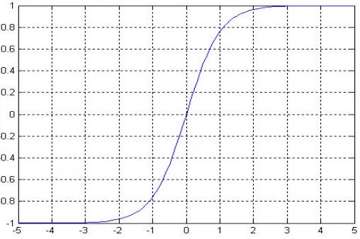
Only two of the above-mentioned transfer functions are used in this thesis, namely, the hyperbolic-tangent and the linear functions. The former has the form:

u u

u u i

e e

output ₋

−

+ −

= (3.2)

where u =g⋅input_i. g=1/T is the gain of the function, where T is the threshold. The gain determines the skewness of the function around 0. The function has continuous values in the interval [-1,1]. The hyperbolic-tangent function is commonly used in multilayer networks that are trained using the backpropagation algorithm, in part because this function is differentiable. The graph is shown in the following the figure below:

(31)

Because of its ability to map values into positive as well as negative regions, this function is used throughout Matlab implementation in this thesis.

A linear function has the form:

i

i g input

output = ⋅ (3.3)

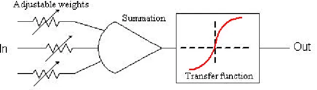
It should be pointed out that Matlab names the hyperbolic tangent tansig, which has the same shape, and the linear function purelin. Figure 3.2 below depicts the overall picture of the input, transfer function, and output of a typical multiple-input neuron.

Choice of the appropriate transfer function is made in the network design phase, still allowing the change of threshold value (T) and gain (g). The best transfer function is usually obtained by experimenting on a particular problem.

Figure 3.2 Multiple -input neuron

3.1.4 Type of Learning

(32)

with only input patterns. Without desired responses, the network has no knowledge about whether or not its resulting outputs are correct. As a result, the network has to self-organize (cluster) the data into similar classes by adjusting its weights so that the clustering improves. This type of learning is commonly used for pattern recognition problems and clustering. Kohonen's self-organizing network is based on unsupervised learning.

Every NN goes through three operative phases:

1) learning (training) phase - network learns on the training sample, the weights are being adjusted in order to minimize the objective function (for example the RMS or root mean square error),

2) testing phase - network is tested on the testing sample while the weights are fixed, 3) operative (recall) phase - NN is applied to the new cases with unknown results

(weights are also fixed).

Learning Rules

A learning rule represents the formula that is used in NN to adjust the connection weights among neurons. Among various learning rules developed so far, four of them are most commonly used: Delta rule, Generalized Delta rule, Delta-Bar-Delta and Extended Delta-Bar-Delta rules, and Kohonen's rule.

1) Delta rule

(33)

values. The aim is to minimize the sum of square error, where error is defined as the difference between the computed and the desired output of a neuron, for the given input data. The Delta rule equation is:

i cj

ji y e

w = ⋅ ⋅

∆ η , (3.4)

where ∆w_ji is the adjustment of the connection weight from neuron jto neuron

icomputed by:

old ji new ji

ji w w

w = −

∆ , (3.5)

cj

y is the output value computed in the neuron j; ei is the raw error computed by:

di ci

i y y

e = − , (3.6)

η is the learning coefficient, and y_di is the desired (actual) output that is used to compute

the error.

The raw error in formula (3.6) is very rarely backpropagated; more often other error forms are used. In a classical Backpropagation NN, the error is backpropagated through the network using the gradient descent algorithm described in section 3.2.1. The gradient component of the global error E backpropagated into a connection k is:

k k k

w E

∂ ∂ =

δ , (3.7)

(34)

global minimum. Since the problem is mainly apparent in the Backpropagation algorithm, it will be discussed in detail later in the text together with suggested solutions.

2) Generalized Delta rule

Generalized delta rule is obtained by adding a derivation of input neurons into the Delta rule equation such that weight adjustment is computed according to the formula:

) ( i i cj

ji y e f I

w = ⋅ ⋅ ⋅ ′

∆ η , (3.8)

where f′(I_i) is the derivative of the input I_i into neuron i. This rule is appropriate to be used with non-linear transfer functions.

3) Delta-Bar-Delta and Extended Delta-Bar-Delta rules

(35)

i cj k k

ji y e

w = ⋅ ⋅

∆ ( ) η . (3.9)

Weight increments are conducted linearly, while decrements are conducted geometrically. Despite its advantages over the classical Delta rule, Delta-Bar-Delta has some limitations, such as lack of a momentum term in the learning equation and large “jumps” that can skip important regions of the error surface due to the linear increments of the learning rates. This cannot be prevented by slow geometrical decrements.

In order to overcome these shortcomings, Extended-Delta-Bar-Delta rule (EDBD), proposed by Minai and Williams [30] introduces a momentum term αk, which

also varies with time. The momentum term is used to prevent the network weights from saturation (see details in section 3.2.1), and the EDBD rule enables local dynamic adjustment of this parameter, such that the learning equation becomes:

1 ) ( ) ( − ∆ + ⋅ ⋅ = ∆ t k ji k i cj k t k

ji y e w

w η α , (3.10)

where αk is the momentum of the connection k in the network and t is the time point in

which the weights of the connection k are adjusted. Both the learning rates and the momentum term are adjusted exponentially, not linearly or geometrically as in DBD. The magnitudes of the exponential functions are the weighted gradient components

k

δ (equation 3.7), which makes a larger increase in the areas of a small error curvature,

and a smaller one in the areas of large curvature, thereby preventing the big “jumps” present in the DBD rule.

(36)

4) Kohonen's rule

Since Kohonen's network does not learn on known outputs, the weights are adjusted using the input into the neuron i:

ji i ji extinput w

w = ⋅ −

∆ η , (3.11)

where extinputi is the input that neuron i receives from the external environment.

Kohonen's rule is used in Kohonen's self-organizing network. Details concerning learning equations are given in section 3.3.2.

3.1.5 Other Parameters for NN Architecture Design

According to the number of layers, NN architectures can be one-layered (with the output layer only) or multi-layered (with one or more hidden layers additionally). The number of necessary hidden layers should be experimentally determined. It is to be expected that more hidden layers should be used for approximating a very complex linear function, although it is proven that two-layered NNs can approximate any non-linear function as mentioned earlier.

NNs can be divided into:

a) deterministic networks - when a neuron reaches a certain activation level, it sends impulses to other neurons (it "fires"),

(37)

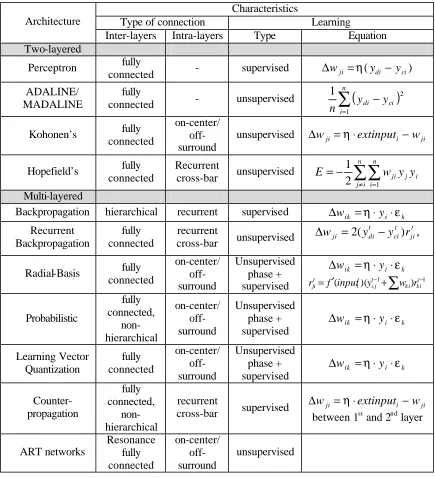
Characteristics

Type of connection Learning Architecture

Inter-layers Intra-layers Type Equation Two-layered

Perceptron fully

connected - supervised ∆wji =η(ydi − yci)

ADALINE/ MADALINE

fully

connected - unsupervised

∑

(

)

= − n i ci di y y n 1 2 1

Kohonen’s fully connected

on-center/ off-surround

unsupervised ∆w_ji =η⋅extinput_i −w_ji

Hopefield’s fully connected

Recurrent

cross-bar unsupervised

∑∑

≠ = − = n i j n i i j jiy y

w E 1 2 1 Multi-layered

Backpropagation hierarchical recurrent supervised ∆w_ik =η⋅y_i⋅ε_k

Recurrent Backpropagation

fully connected

recurrent

cross-bar unsupervised

, ) (

2 t_di _cit _jit

ji y y r

w = −

∆

Radial-Basis fully connected on-center/ off-surround Unsupervised phase + supervised k i ik y

w =η⋅ ⋅ε

∆

∑

−

− ₊

′

= 1 1

) )(

( ki kit

t cj t i t

ji f input y w r r Probabilistic fully connected, non-hierarchical on-center/ off-surround Unsupervised phase + supervised k i ik y

w =η⋅ ⋅ε

∆ Learning Vector Quantization fully connected on-center/ off-surround Unsupervised phase + supervised k i ik y

w =η⋅ ⋅ε

∆ Counter-propagation fully connected, non-hierarchical recurrent

cross-bar supervised

ji i ji extinput w

w = ⋅ −

∆ η

between 1st and 2nd layer

ART networks Resonance fully connected on-center/ off-surround unsupervised

Table 1. Neural Network Architectures

NNs can also be classified as

a) static networks (receive inputs in one pass),

(38)

NN learning can be:

a) batch learning - network learns only in the learning phase, in other phases weights are fixed,

b) on-line learning - network also adjusts its weights in the recall phase.

Table 1 [31] above shows a brief overview of well-known NN architectures according to the above parameters for architecture design. Further text presents detailed description of various NN architectures.

3.2 Backpropagation Network

Back-propagation (BP) [15], [19], [37] is a multi-layer neural network using sigmoidal activation functions. Originally developed by Paul Werbosin in 1974, extended by Rumelhart, Hinton, and Williams in 1986, this was the first network with more than one hidden layer. Its role was primarily to solve the "credit assignment" problem imposed by the Perceptron network, which is the problem of assigning the adjustments of parameters or connection weights. The suggested solution was to localize the error by computing it at the output layer and backpropagating the error to each hidden layer such that weights of connections are adjusted until the input layer is reached.

(39)

of local minima. In this thesis implementation, second order methods will not be used, but some parameter adjustments to avoid the main shortcomings of the classical Backpropagation algorithm will be implemented.

Architecture of the network

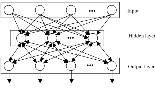
The network is made up of an input layer, at least one hidden layer, and an output layer. Nodes in each layer are fully connected to those in the layers above and below. Each connection is associated with a synaptic weight. Typical backpropagation architecture is presented in Figure 3.3 (for clarity reasons only 1 hidden layer is shown):

Input

Hidden layer

Output layer

...

Figure 3.3: Architecture of Backpropagation Neural Network

Data flow through the network can be briefly described in few steps:

1) from the input to the hidden layer: the input layer loads data from input vector X, and sends them to the first hidden layer,

(40)

3) as information propagates through the network, all the summed inputs and output states are computed in each processing unit,

4) in the output layer: for each processing unit, the scaled local error is computed and used to determine the weight increment or decrement,

5) Backpropagation from the output back to the hidden layers: the scaled local error and weight increments or decrements are computed for each layer backwards, starting from the output layer and ending at the first hidden layer, and the weights are updated.

Computation in the network

When the input layer sends data to the first hidden layer, each hidden unit in the hidden layer receives weighted input from the input layer (initial weights are set randomly) according to the formula [15]:

∑

_⋅

−

=

i

s i s ji s

j

w

x

I

[ ] [ ] [ 1] _, _(3.11)

where I[_js] is the input to neuron j in layer s, w[_jis] is the connection weight from neuron

j to neuron iin layer s, and x_i[s−1] is the output of the neuron i in layer s−1. Units in the hidden layer transfer those inputs according to the formula:

( )

s j i

s i s ji s

j f w x f I

x =

  



 _⋅

=

∑

[ ] [ −1] ]

[

, (3.12)

(41)

reached. At the output layer, the network output is compared to the desired (real) output, and the global error E is determined as:

=

∑

−

k

k x

d

E ( ) ,

2

1 2

(3.13)

where dk is the desired (real) output, xk is the output of the network, and k is the index

for the component of the output, i.e., the number of output units. Each output unit has its own local error e whose raw form is (d_k −x_k), but what is backpropagated through the networks is the scaled error in the form of a gradient component:

) ( ) ( / / / ( ) ) ( k k k k k k x k x

k E I E x x I d x f I

e =−∂ ∂ =−∂ ∂ ⋅∂ ∂ = − ⋅ ′ . (3.14)

The objective of the Backpropagation learning process is to minimize the above global error by backpropagating it into the connections through the networks backwards until the input layer is reached. By modifying the weights, each connection in the network is corrected in order to achieve a smaller global error. The process of incrementing or decrementing the weights (learning) is done by using a gradient descent rule: ), / ( [] ] [ s ji s

ji E w

w =− ⋅ ∂ ∂

∆ η (3.15)

where η is the learning coefficient. To compute partial derivations in the above equation we can use (3.14), which gives:

. ) / ( ) / (

/∂ [] = ∂ ∂ [ ] ⋅ ∂ [] ∂ [ ] =− []⋅ [−1]

∂ s i s j s ji s j s j s

ji E I I w e x

w

E (3.16)

When the above result is included in formula (3.15), the weight adjustment is , ] 1 [ ] [ ] [ ₌ _⋅ _⋅ − ∆ s i s j s

ji e x

(42)

which leads to the main problem of setting the appropriate learning rate.

There are two mutually conflicting guidelines for determining η. The first guideline is to keep η low because it determines the area in which the error surface is locally linear. If the network aims to predict high curvatures, that area should be very small. However, a very low learning coefficient means very slow learning. In order to resolve this conflict, the previous delta weights in time (t−1) are added in equation (3.17), so that the current weight adjustment is:

,

] [ 1 ]

1 [ ] [ ]

[ t s

ji s

i s j s

ji e x w

w = ⋅ ⋅ − + ⋅∆ −

∆ η α (3.18)

(43)

Improvements of Standard Backpropagation Network Learning Rules

Since one of the main disadvantages of Backpropagation is its slow learning, much effort has been expanded in improving the learning rules and other parameters. Some of the achievements are [19], [38]:

• Delta-Bar-Delta (DBD) rule - a learning rule that uses past values of the gradient to find the local curvature of the error and allocates a different learning coefficient to each connection in the network,

• Extended Delta-Bar-Delta (EDBD) rule - besides using a different learning rate for each connection, it uses a different momentum term for each connection (equations are described in section 3.1.4),

• QuickProp and MaxProp - learning rules that use quadratic estimation heuristics to determine the direction and step size for the weight changes,

• Resilient Backpropagation (Rprop) - A local adaptive learning scheme that eliminates the harmful effect of having a small slope at the extreme ends of the sigmoid "squashing" transfer functions.

(44)

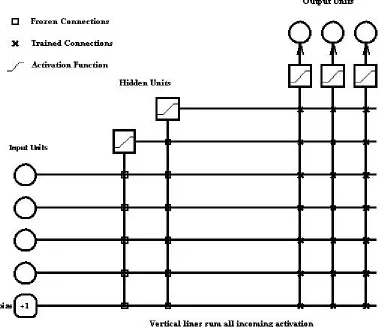
Resilient Backpropagation (Rprop)

Multilayer networks typically use sigmoid transfer functions in the hidden layers. Sigmoid functions are characterized by the fact that their slope must approach zero as the input gets large. This causes a problem when using steepest descent to train a multilayer network with sigmoid functions, since the gradient can have a very small magnitude; and therefore, cause small changes in the weights and biases, even though the weights and biases are far from their optimal values.

The purpose of the Rprop [38] training algorithm is to eliminate these harmful effects of the magnitudes of the partial derivatives. Only the sign of the derivative is used to determine the direction of the weight update; the magnitude of the derivative has no effect on the weight update. The size of the weight change is determined by a separate update value. The update value for each weight and bias is increased by a factor delt_inc whenever the derivative of the performance function with respect to that weight has the same sign for two successive iterations. The update value is decreased by a factor delt_dec whenever the derivative with respect that weight changes sign from the previous iteration. If the derivative is zero, then the update value remains the same. Whenever the weights are oscillating the weight change will be reduced. If the weight continues to change in the same direction for several iterations, then the magnitude of the weight change will be increased.

Dealing with Local Minima and Overtraining

(45)

network (gradient descent optimization), learning can stick in a local minimum and minimize the error only locally. There are a number of solutions for this problem. Some of them are deterministic and use second order equations to compute the error, while others are stochastic, and rely on random numbers rather than on equations. One of the stochastic methods for avoiding local minima is simulated annealing.

Overtraining is the universal problem for all types of NN algorithms. It occurs when the network learns the training sample perfectly, but is not able to generalize on the test sample. One of the main still unanswered questions on how long it takes to learn can be approached in the following ways [33]:

• cross validation using the validation sample to determine when to stop learning. The training will continue as long as the error on the validation sample improves. When it does not improve, the training will stop. Such iterative procedure is usually called the "Save best" procedure, which alternatively trains and tests the network until the performance of the network does not improve for n number of iterations. After the best network is selected, it is tested on a new test sample to determine its generalization ability (since this method is used in our experiments, it is described in detail in section),

• adding bias and random error in parameter estimates,

• jackknifing,

• bootstrapping, and others.

Input Parameters to Build the Network

(46)

The number of hidden units can be statically set to a fixed number or dynamically optimized during the learning phase of the NN. In this implementation, one node is used and another node added if the goal is not met (this is discussed in detail in section 4).

2) learning coefficients Learning coefficients can be set:

• statically and globally for the whole network in a way that coefficients do not change during the learning process,

• statically and locally by setting a different learning rate for each hidden layer or connection,

• dynamically and globally by changing the global learning rate while the learning process improves,

• dynamically and locally by assigning a different learning rate to each connection in the network and changing them during the learning process.

3) Bias (F'Offset)

As explained in the previous section, this parameter prevents the network from saturating the weights.

4) learning rule

This is a procedure for modifying the weights and biases of the network. 5) transfer function

The choice of a transfer function is made according to its ability to map into positive as well as negative regions. This transfer function is often used in image compression.

(47)

Input values are scaled between -1 and 1. Because positive and negative values in the input variables are desired, this option is used in the thesis implementation.

7) MinMax table

Inputs to the network are preprocessed using the so-called Minmax table created from the training data. Such a table consists of minimum m_i(i=1,...,n) and maximum

) ,..., 1 (i n

M_i = values for each of the n variables in the network, where n is the sum of the number of input variables I and the number of desired output variables D. Those values together with the network range parameters (specified in the I/O set of parameters) are used to scale each input and output variable according to the formula:

, ) ( ) ( ) ( i i i i i i i i i i m M R m r M x r R s − ⋅ − ⋅ + ⋅ −

= (3.19)

where si is the scaled new value for the variable ,i Ri is the upper limit of the network

range for inputs (or outputs), and ri is the lower limit of the network range for inputs (or

outputs). Such a scaling process is necessary because of the output range of transfer functions used in the networks. For example, the hyperbolic tangent function has the output range of [-1,1], and therefore the inputs to and outputs of the network need to be mapped into the same range. Upon completion of the learning process, output values of the network are rescaled, so that original real values are presented to the user.

8) epoch

(48)

3.3. Radial-Basis Function Network

A Radial-Basis function network (RBFN), proposed by M.J.D. Powel [34], is a general-purpose network which can be used in the same situations as a Backpropagation network for prediction as well as for classification problems. Since it uses a radially symmetric and radially bounded transfer functions in its hidden layer, it is a general form of probabilistic and general regression networks. It overcomes some disadvantages of Backpropagation such as slow training time and the local minima problem, but requires more computation in the recall phase in order to perform function approximation or classification.

Computation in the Network

Any network using radially symmetric hidden units belongs to the class of Radial-Basis Function networks. A pattern of hidden units is radially symmetric [30], if it: (a) has a "center", i.e. an input vector stored in the weight vector between the input and the hidden layer, (b) has a distance measure which determines the distance of each input vector from the center, (c) has a transfer function which maps the output of the distance function.

(49)

their shape, and the method used for determining the associative weight matrix W [35]. Some existing strategies for training RBFNs can be classified as follows:

1) RBFNs with a fixed number of centers selected randomly from the training data,

2) RBFNs with unsupervised procedures for selecting a fixed number of Radial-Basis Function centers,

3) RBFNs with supervised procedures for selecting a fixed number of Radial-Basis Function centers.

The above strategies all have the same disadvantage: the number of centers must be determined in advance. To overcome this shortcoming, several authors suggested algorithms, such as the growing cell structure (GCS) proposed by Fritzke, distribution of radial-basis functions with space-filling curves proposed by Whitehead and Choate, dynamic decay adjustment (DDA) algorithm proposed by Berthold and Diamond, and merging two prototypes at each adaptation cycle. All the above algorithms involve either cascade or pruning principles [39].

The focus below will be on the RBFN algorithm proposed by Moody and Darken [30], which uses Euclidean distance and a Gaussian transfer function in the hidden layer. The input to the hidden units is computed according to the formula [37]:

∑

= − = − = N i ki i k

k X c X c

I

1

2

, )

( (3.20)

where c is the center. The output is computed using a Gaussian transfer function:

(

)

, ) ( 2 2     = − = k k I e c x x

(50)

where the center c is determined by a clustering algorithm and by the nearest neighbor technique.

Architecture of the Network

The RBF learning algorithm can be briefly described as follows:

- training starts in the hidden layer with an unsupervised learning algorithm in order to determine the center,

- training continues in the output layer with a supervised learning algorithm in order to compute the error,

- simultaneous application of a supervised learning algorithm to the hidden and output layers to fine-tune the network.

A common RBFN architecture is shown in the figure below.

Input

Hidden layer (pattern units)

Output layer

...

Summation

(51)

Learning through the architecture can be described in the following steps:

1) from the input to the hidden layer: Clustering phase. In this phase the incoming weights to the prototype layer learn to become the centers of clusters of input vectors using a dynamic algorithm.

2) in the hidden layer: The radii of the Gaussian functions at the cluster centers are computed using a 2-nearest neighbor technique. The radius of a given Gaussian is set to the average distance to the two nearest cluster centers.

3) in the output layer: Error is computed at the output layer using one of the learning rules. It is also possible to include one additional hidden layer to improve learning.

Application of the Network

Karayiannis and Weigun [35] give a brief overview of the previous usage of a Radial-Basis network that starts with Broomhead and Lowe year who first implemented this network and showed how it models nonlinear relationships. The ability of a RBFN with one hidden layer to approximate any nonlinear function is proved by Park and Sandberg. Then Michelli showed how this network could produce an interpolating surface, which passes through all the pairs of the training set.

Advantages of a RBFN can be briefly summarized as follows: - fast training,

(52)

- hidden unit can be interpreted as a density function for the input vectors and thus measures the probability that a new vector is a member of the same distribution as others in the input space.

Disadvantages:

- despite fast learning, it can be slower than Backpropagation in the recall phase,

- since the initial learning phase of a Radial-Basis Function network is the unsupervised clustering phase, some discriminatory information could be lost in this phase,

- it is difficult to determine the optimal number of prototype units [35]. The authors who propose several ways to overcome this disadvantage: a Growing Radial-Basis (GRBF) network that starts with a small number of prototypes at each growing cycle and grows in the training process by splitting of the prototypes in each cycle. They also suggest two criteria to determine which prototype to split, and test different hybrid learning schemes for incorporating existing learning schemes into RBFN, such as unsupervised learning for clustering, learning vector quantization, and linear neural networks, with very satisfactory results. The authors also propose a supervised learning scheme based on minimization of the localized class-conditional variance.

The RBFN uses the same input parameters as the Backpropagation network

3.4 General Regression Network

(53)

classification problems. GRNN can be used for system modeling and prediction, with the special ability to deal with sparse and nonstationary data. Its disadvantages, such as memory intensiveness and time-intensiveness in the recall phase, are not limiting factors for today's fast computers.

GRNN is designed to perform a nonlinear regression analysis. If f(x,z) is the probability density function of the vector random variable x(input vector) and its scalar random variable z(measurement), then the computation in GRNN consists of calculating the conditional mean E(z|x)of the output vector, given by [37]:

. ) , ( ) , ( ) | (

∫

∞ ∞ − ∞ ∞ − = dz z x f dz z x zf x z E (3.22)

The joint probability density function (pdf) f(x,z) is required to compute the above conditional mean. GRNN approximates the pdf function from the training vectors using Parzen window estimation, a nonparametric technique that approximates a density function by constructing it out of many simple parametric pdfs [40]. Parzen windows are Gaussian with a constant diagonal covariance matrix:

(54)

where P is the number of sample points xi, N is the dimension of the vector of sample points xi, σ is a smoothing constant, and Di is the Euclidean distance between xand

i

x computed by:

(

)

, 1 2

∑

= − = − = i i i

i x x x x

D (3.24)

where N is the number of input units to the network, σ is the width parameter which satisfies the following asymptotic behavior as the number of Parzen windows P becomes large:

∞ = ∞

→

lim (P P)

P σN and (3.25)

0 ) (

lim ∞ =

→

 P P

P σN

or when = ₍ _/ ₎ ,0≤ E<1,

P S

N E

σ (3.26)

where S is the scale and, N is the number of input units. When estimated pdfs are inserted into equation (3.22), the following formula for computing each component z_jis obtained . ) ( 1 2 1 2 2 2 2 2

∑

= − = − = P i D P i D i j j i i e e z x z σ σ (3.27)

Since computation of Parzen the estimation is time consuming when the sample is large, a clustering procedure is often incorporated in GRNN. According to this procedure, for

any given sample xi, instead of computing a new Gaussian kernel

2 2

2σ

i

D

(55)

kernel is found, and the old closest kernel is reused. Such an approach transforms the equation (3.27) for z_j, into:

, ,..., 1 , ˆ 2 2 2 2 2 1 1 2 M j e B e A z i i D P i i P i D i

j = =

    − = =         −

∑

σ σ (3.28) where j i i

i A k A k z

A ≡ ( )= ( −1)+ and B_i ≡B_i(k) =B_i(k−1)+1. (3.29)

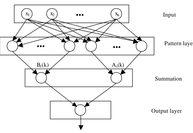
Architecture of the Network

The network consists of the input layer, the pattern layer and the output layer (see Figure 3.5). There is also an additional summation/division layer whose function will be explained later. The process of network learning is conducted as follows:

1) from the input layer to the pattern layer: training vector X is distributed from the input layer to the pattern layer, and the connection weights from the input layer to the th

k unit in the pattern layer store the center X_i of the th

k Gaussian kernel.

2) in the pattern layer: The summation function for the kth pattern unit computes the Euclidean distance Dk between the input vector and the stored center Xi and transforms

it through the exponential function 2

2

2σ

i

D

e− . Then B coefficients are set as connection weights from the pattern layer to the first unit in the summation/division layer, and A

(56)

Input

Pattern layer

Summation and division

...

x1 x2 x3 xn

...

Bi(k) A1(k) Ai(k) Am(k)

z1 zj zm Output layer

Figure 3.5: Architecture of GRNN

3) in the summation/division layer: the summation function of this layer (which is the standard weighted sum function) computes the denominator of equation (3.27) for the first unit (j), then the numerator for each next unit (j+1). To compute the output zˆj(x),

the summation of the numerator is divided by the summation of denominator and such output is forwarded to the output layer (note that the first unit of the summation layer does not generate the output).

(57)

Application of the Network

Because of its generality, GRNN can be used in various problems such as prediction, plant process modeling and control, general mapping problems, or for other problems where nonlinear relationships exist among inputs and output [37]. One of the main advantages of GRNN is the ability to deal with nonstationary data (time series data whose statistical properties change over time). This ability is obtained by modifying the computation of theB and A coefficients in equation (3.27) such that a time constant is introduced in terms of number of training vectors, as an indication of how fast the time series changes its characteristics.

It can be concluded from the above description of GRNN that it is especially adaptable to (a) nonstationary and sparse data and (b) stationary but noisy data.

1) number of input, pattern and output layer units.

2) summation function in the pattern unit (Euclidean, City Block, or Projection). 3) τ - time constant

τ is defined in terms of training vectors, and should be adjusted according to the degree of nonstationarity present in the data. A smaller time constant will cause the network to forget the previous cases faster.

4) θ - reset factor

(58)

5) radius of influence

This is a clustering mechanism for determining the limit of the Euclidean distance by which an input vector will be assigned to a cluster. The input vector will be assigned to a cluster if the cluster center is the nearest center to the input vector, or if the cluster center is closer than the radius of influence. If the input vector does not satisfy the above conditions, a new center is computed for the vector.

6) sigma scale (S) and sigma exponent (E)

S and E values are used in computing the Parzen window width in formula (3.26).

3.5. Modular Network

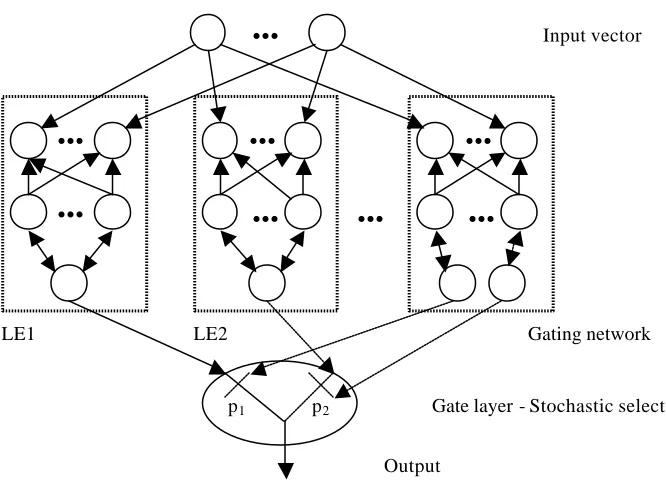
Proposed by Jacobs, Jordan, Nowlan and Hinton (1991), this network is a system of many separate networks (usually Backpropagation). Each of them learns to handle a subset of the complete set of training cases. It is therefore able to improve the performance of Backpropagation when the training set can be naturally divided into subsets that correspond to distinct subtasks.

(59)

suggested that the final output of the whole system is a linear combination of the outputs of the local experts, Jacobs et al. [41] use a stochastic selector and compute the error according to the formula:

, 2

∑

− = − = i c i c c i c i c c o d p o d

E (3.30)

where o_ic is the output vector of expert i in case c, p_ic is the proportional contribution of expert i on the combined output vector, and c

d is the desired output vector in case c. In such a process each local expert produces the whole output, and the goal of one local expert is not directly affected by the weights of the other local experts. Although some indirect coupling can occur if the gating network alters the responsibilities from one local expert to another, still the sign of the local expert error remains uninfluenced. The number of local experts in the network is determined in advance, based on the assumption of the number of subsets or local regions in the input space of the sample. Each local expert is a feedforward network and all experts have the same number of input and output units. Local experts as well as the gating network receive the same input. Of course, their output differs. Output of the gating network is the probability [41]:

, ) ( ) (

∑

= i x x j _i j e e

p (3.31)

where xj is the total weighted input received by output unit j of the gating network, and

j

p is the probability that the switch will select the output from local expert j. This

output is normalized to sum to 1. The output of the local experts yi is then corrected by

Image Compression Using Cascaded Neural Networks

ScholarWorks@UNO

ScholarWorks@UNO

Image Compression Using Cascaded Neural Networks

Image Compression Using Cascaded Neural Networks

CASCADED NEURAL NETWORKS

ACKNOWLEDGMENTS

TABLE OF CONTENTS

LIST OF TABLES

LIST OF FIGURES

ABSTRACT

CHAPTER 1

Introduction

CHAPTER 2

Techniques for Image Compression

∑

∑

∑ ∑

CHAPTER 3

Artificial Neural Network Technology- an Overview

(

)

∑

∑

(

)

∑∑

∑

...

...

...

∑

⋅

=

w

x

I

( )

∑

∑

∑

(

)

...

...

∫

∫

(

)

∑

∑

∑

∑

∑

...

...

...

...

...

∑

∑

_⋅