VOLUME 37, ARTICLE 13, PAGES 363
,
416
PUBLISHED 16 AUGUST 2017
http://www.demographic-research.org/Volumes/Vol37/13/ DOI: 10.4054/DemRes.2017.37.13
Research Article
Birth spacing, human capital, and the
motherhood penalty at midlife in the United
States
Margaret Gough
© 2017 Margaret Gough.
This open-access work is published under the terms of the Creative Commons Attribution NonCommercial License 2.0 Germany, which permits use, reproduction, and distribution in any medium for noncommercial purposes, provided the original author(s) and source are given credit.
1 Introduction 364
2 Background 365
2.1 Labor force participation patterns of mothers in the United States 365
2.2 Policy context 366
2.3 Human capital theory 367
2.4 Selection 370
2.5 Contributions 371
3 Method 373
3.1 Data and sample 373
3.2 Measures 374
3.2.1 Dependent variables 374
3.2.2 Independent variables 375
3.2.3 Control variables 375
3.3 Analytic strategy 378
3.3.1 Estimation 380
4 Results 381
4.1 Predictors of birth spacing 384
4.2 Birth spacing and labor market outcomes (Hypothesis 1) 384 4.3 Age at birth, human capital, and labor market outcomes
(Hypothesis 2) 385
4.4 Heterogeneous effects by age at first birth and education
(Hypothesis 3) 387
4.5 Description of supplemental analyses 391
5 Discussion 392
6 Conclusions 394
7 Acknowledgements 397
References 398
Birth spacing, human capital, and the motherhood penalty
at midlife in the United States
Margaret Gough1
Abstract
BACKGROUND
Researchers have examined how first-birth timing is related to motherhood wage penalties, but research that examines birth spacing is lacking. Furthermore, little research has examined the persistence of penalties across the life course.
OBJECTIVE
The objective is to estimate the effects of birth spacing on midlife labor market outcomes and assess the extent to which these effects vary by education and age at first birth.
METHODS
I use data from the United States from the 1979–2010 waves of the National Longitudinal Survey of Youth 1979 and dynamic inverse probability of treatment weighting to estimate the effects of different birth intervals on mothers’ midlife cumulative work hours, cumulative earnings, and hourly wages. I examine how education and age at first birth moderate these effects.
RESULTS
Women with birth intervals longer than two years but no longer than six years have the smallest penalties for cumulative outcomes; in models interacting the birth interval with age at first birth, postponement of a first birth to at least age 30 appears to be more important for cumulative outcomes than birth spacing. College-educated women benefit more from a longer birth interval than less educated women.
CONCLUSIONS
Childbearing strategies that result in greater accumulation of human capital provide long-run labor market benefits to mothers, and results suggest that different birth-spacing patterns could play a small role in facilitating this accumulation, as theorized in past literature.
CONTRIBUTION
I contribute to the demographic literature by testing the theory that birth spacing matters for mothers’ labor market outcomes and by assessing the effects at midlife rather than immediately following a birth.
1. Introduction
Nearly 80% of mothers in the United States bear two or more children (Dye 2008), and a majority of these mothers are also employed (Bureau of Labor Statistics 2013). The labor market penalties experienced by mothers (the “motherhood penalty”) are well known, and some evidence suggests that the labor market costs of a second child are even greater than those of a first child (Anderson, Binder, and Krause 2003; Budig and England 2001; Loughran and Zissimopoulos 2009). Yet, while we know women in the United States can mitigate the cost of a first child by postponing motherhood, we know virtually nothing about whether and how women can mitigate the costs of a second (or higher-order) child. In this study, I investigate whether birth spacing (the interval between the first and second births) plays a role in explaining the second-child penalty for US mothers. Specifically, I examine the second-child penalty accrued by age 45. By focusing on the second-child penalty at midlife, I provide insight into the long-run financial being of mothers with multiple children, especially how financial well-being may vary according to childbearing patterns.
The timing of first births and the spacing of subsequent children are intimately linked for biological reasons – the longer a woman postpones a first birth, the less time she has for bearing additional children. As such, the effects of birth timing and birth spacing may be confounded in existing estimates of the motherhood penalty. For example, if spacing one’s children close together is good for women’s labor market outcomes, as Ross (1974) and Mincer and Polachek (1974) have argued in their classic studies, and women who begin bearing children at later ages also tend to space their children close together (Troske and Voicu 2013), the reported financial benefits to postponing a first birth found in previous research will be overstated, since these benefits will derive from the spacing pattern as well as first-birth timing.
Understanding the relevance of birth spacing is important in the contemporary context because US women report that they want to have two children on average (Bongaarts 2002), but they also spend considerably longer in full-time, full-year work than previous generations of women, and they lack the social welfare supports that many other countries offer to reduce the conflict between paid labor and childbearing (Blau and Kahn 2013; Karimi 2014). Furthermore, their earnings comprise an increasingly large share of household income. While the median contribution of wives’ earnings to family income was 26.7%, in 1980, the contribution has topped 36% since 2007, and the proportion of households headed by single mothers has also grown (Bureau of Labor Statistics 2013). Because birth-spacing patterns vary across different demographic characteristics and different social and policy contexts, differential birth spacing could be one contributor to inequalities in financial well-being across groups of women or across country contexts. In addition, spacing may be more influenced by family policies than first-birth timing, potentially suggesting a mechanism for policy change if certain spacing patterns are determined to be detrimental to women’s long-run earnings or work experience.
2. Background
2.1 Labor force participation patterns of mothers in the United States
later, and married women are the most likely to have returned to the labor force within nine months of the first birth (Han et al. 2008), while women with low levels of resources and financial difficulties are more likely to return to the labor force within two months of the first birth (Han et al. 2008; National Partnership for Women and Families 2013).
2.2 Policy context
The policy context in which mothers in the United States make decisions about continued labor force participation differs considerably from the context in most other highly developed countries. For example, it was not until 1993 that the United States introduced the Family Medical Leave Act (FMLA), which mandated up to 12 weeks of unpaid leave for childbearing or family care over a 12-month period, and the act only applies to certain eligible employees (Laughlin 2011). There remains no federally mandated paid childbearing leave in the United States. As such, women taking leave under FMLA for a new child average only 58 days of leave (National Partnership for Women and Families 2013). Additionally, US women appear to experience wage penalties for motherhood, only part of which can be explained by reductions in work experience. This policy context contrasts considerably with countries such as Germany or Sweden. Germany, for example, provides maternity leave and maternity benefits (fully paid), parental leave of up to three years with job protection, and child-rearing benefits that are government transfers (Bergemann and Riphahn 2015). But labor force participation rates of mothers of young children are relatively low because the availability of childcare outside of the home is very limited (Brehm and Buchholz 2014), and researchers have estimated motherhood wage penalties of 18% (Gangl and Ziefle 2009). Sweden, on the other hand, combines a relatively long and generous parental leave period with widely available subsidized public childcare. As such, about 50% of Swedish mothers return to the labor market within three years of a first birth (Aisenbrey, Evertsson, and Grunow 2009), and some research indicates that the wage penalties for taking leave are minimal (Albrecht et al. 1999).
2.3 Human capital theory
motherhood penalty literature two of the common explanations for the penalty are most plausible as mechanisms through which birth spacing could affect women’s outcomes: human capital accumulation and productivity, and selection. Lower investment in human capital (e.g., education, work experience, tenure) generally explains a portion of the motherhood penalty in the empirical literature (typically about 50%), but much of the penalty remains unexplained after accounting for human capital (Anderson, Binder, and Krause 2003; Budig and England 2001). Women may also suffer depreciation of their skills during periods out of the labor market (Mincer and Polachek 1974), which will also lower wages upon return to the labor force. Skill depreciation is greater for women with larger amounts of job- or employer-specific human capital compared to women with larger amounts of other types of human capital (Mincer and Polachek 1974).
It could also be the case that mothers are less productive in the workplace and this lower productivity results in the motherhood penalty. Becker (1985) argued that individuals have only a limited amount of effort to expend, and mothers will use more of their effort at home, leaving less available for paid work. This translates into lower on-the-job productivity, which results in lower wages, all else being constant. Unfortunately, productivity is largely untested in the literature and cannot be tested in this study either.
Women who return to the labor market after having a first child and before having a second child accumulate more work experience and tenure, which leads to higher wages over time (Troske and Voicu 2013). It is also likely to reduce the depreciation of human capital women experience from time out of the labor market for childbearing. From a productivity perspective, spacing children close together intensifies the early child-rearing period, which may make remaining attached to the labor force impossible, thereby hurting women’s long-term economic growth. On the other hand, working part-time or shifting to the “mommy track” may halt women’s career progress (Noonan and Corcoran 2004; Stone and Lovejoy 2004). Thus, if a longer birth interval means that women spend more time in part-time work, rather than returning to full-time work between births, the return to the labor market between children may be no more valuable than having two births close together and only returning to work (full-time) after the second child is born. For example, my informal calculations, based on Waldfogel’s (1997) finding that part-time work carries a 10% penalty in the United States, indicate that working four years part-time would net the average woman only about 90% of the income of a comparable woman working two years full-time.
Neumark 1993), greater market productivity (Troske and Voicu 2013), and a potential for higher wage growth. They may also experience less depreciation of human capital than earlier childbearers if depreciation costs decline with increased experience (Miller 2011). Greater human capital accumulation may also reduce the amount of time women take off after having a child (Herr 2012).
A recently published thesis chapter by Karimi (2014) is one of the few studies to address these issues as they relate to labor income and wages over the longer term, as I consider here. She studied income and wages 15 years after the second birth using Swedish register data and instrumenting for birth spacing using miscarriages. Karimi (2014) hypothesized that postponement of a first birth might not have the same benefits to women in Sweden as it does in the United States because Swedish family policies are universal and generous. She found that women who delay first births in Sweden tend to have the second child faster than those who did not delay. This is potentially problematic, because an increase in spacing between first and second births was associated with increased labor income over 15 years, an increased probability of returning to the labor market between births, increased long-run labor force participation for mothers, and an increase in monthly wages, especially for highly educated mothers (Karimi 2014). These findings are generally consistent with the theoretical predictions presented above, but the postponement evidence contrasts with studies from the United States. However, as discussed above, the Swedish welfare state context differs significantly from the US welfare state context, so it is difficult to know whether the results will hold in the US context.
Another study (Brehm and Buchholz 2014), looking at a sample of mothers in western Germany, found that only highly educated women could continue accumulating labor market prestige after childbearing, and only if they spaced their births close together. Mothers with low education experienced reduced prestige regardless of the spacing of their children. Furthermore, interspersing births with part-time employment was worse for women’s careers than interrupting labor force participation completely. While not specifically focused on labor market earnings or labor force participation per se, Brehm and Buchholz’s (2014) results contradict those of Karimi (2014) and suggest that the type of welfare state (in this case, a male breadwinner/female carer type) may have a substantial role to play in whether short or long spacing is better for women’s long-run labor market outcomes.
although they appear to more commonly space their children close together. By contrast, Peltola (2004) found that longer birth intervals were negatively associated with return to the labor market following a second birth. But Peltola’s results were not disaggregated by prior labor force attachment, which could explain the differences in the results between the two studies.2
Human capital theory indicates the importance of minimizing time out of the labor force, and thus skill depreciation, for optimal labor market outcomes. Returning to work between births is one potential strategy to achieve this ideal, and evidence from Karimi (2014) and Troske and Voicu (2013) shows the potential benefits of spacing births farther apart to facilitate this between-birth labor force participation. Thus, I hypothesize that, because longer spacing may reduce time spent out of the labor market:
Hypothesis 1: The magnitude of the motherhood penalty for a second birth will decline as the birth interval increases.
Postponement of a first birth additionally allows women to temporarily exit the labor force around a birth with greater human capital accumulation and higher wages than an exit occurring at a younger age, and this could help explain the lower motherhood penalties for postponers found in the US literature (e.g., Amuedo-Dorantes and Kimmel 2005; Miller 2011), regardless of birth spacing. Thus, I hypothesize that:
Hypothesis 2a: Women who postpone a first birth to at least age 30 will have smaller motherhood penalties than those who have a first birth before age 30.
Hypothesis 2b: Women with college degrees will have smaller motherhood penalties than those without college degrees.
Finally, postponement and spacing may interact in such a way that longer intervals may amplify the benefits of postponement. If postponement is mainly a proxy for
2 While these studies are useful for providing some insights into the role of birth spacing, they are
greater human capital accumulation, then longer intervals may amplify the benefits of human capital accumulation. I hypothesize that:
Hypothesis 3a:At longer birth intervals, women who postponed a first birth to at least age 30 will have smaller penalties than those who did not postpone to at least age 30.
Hypothesis 3b: At longer birth intervals, women with college degrees will have smaller penalties than those without college degrees.
2.4 Selection
Human capital accumulation is a plausible mechanism for explaining the motherhood penalty, but the motherhood penalty could also arise entirely because of selection. Women may choose to have children at times when their careers are stagnating or their wages are low because it reduces the cost of childbearing. Lundberg and Rose (2000) find some evidence for negative selection of motherhood on this basis. Yet a recent paper by Killewald and Gough (2013) finds no evidence of wage anticipation effects prior to birth in the United States. If anticipation effects exist, birth spacing will affect the motherhood penalty inasmuch as it is related to women’s individual capacity for productivity or their lower labor market position. For example, if some women find that caring for children is so demanding that it requires leaving the labor force temporarily, a rise in a woman’s wages will lead her to postpone having another child until the cost of leaving the labor force declines (Hotz, Klerman, and Willis 1997). This strategy poses a challenge for estimation of causal effects of birth-spacing intervals on future labor market outcomes because past labor market outcomes may influence both the birth-spacing interval and future outcomes. Dynamic models address this causal inference problem, which makes them an invaluable tool for my exploration of the causal effects of birth-spacing intervals.
the extent that such mechanisms are related to observed characteristics they can be accounted for indirectly in a statistical analysis.
The length of a birth interval may also result from unexpected circumstances. For example, either the first or the second birth may be mistimed, or women may have difficulty conceiving a second child, particularly if they postponed their childbearing to the point when their ability to conceive was already declining. These unexpected circumstances, though difficult to analyze, are beneficial from the researcher’s perspective because they suggest that random variation exists (net of selection issues) and this is important for the identification of causal effects.
2.5 Contributions
I estimate the effect of birth spacing on the accumulation of the motherhood penalty for US women’s midlife labor market outcomes. In doing so, I expand my focus beyond the standard outcomes in the motherhood penalty literature to examine cumulative labor market outcomes, in addition to hourly wage penalties. I examine whether penalties that may arise from different birth-spacing patterns are observed even over a long period of time, specifically around age 45. Past research suggests that motherhood penalties persist over time (Karimi 2014; Wilde, Batchelder, and Ellwood 2010), but to date persistence is an understudied issue.
Because of the inherent complications in comparing long-term outcomes among individuals with different times of entry into the labor market, different numbers of spells out of the labor force, and different labor market trajectories, I focus on the midlife outcomes at a single point in women’s lives, at age 45, allowing elements of their previous histories to be absorbed into the net effect I observe at that age. I examine hourly wages for their theoretical importance and because they are the economic outcome of interest in the vast majority of motherhood penalty studies. However, I am also interested in women’s cumulative work behavior and financial well-being. If some women accept a short period out of the labor force, during which they earn no income, in return for higher lifetime earnings than other women who spend more time in part-time work, it would be a mistake to believe that the women who take this part-time out of the labor force are disadvantaged in the long run. Therefore, I examine women’s cumulative work experience and their cumulative earnings by age 45 to better understand potential long-run consequences.
birth interval on the outcomes, using the same techniques as in other motherhood penalty research. This allows me to capture the possibility of penalties incurred across the life course, beyond any evidence I find for penalties measured at age 45.
I use a dynamic potential outcomes framework to estimate the effects of second births at different intervals on midlife outcomes. By introducing a dynamic framework, I can take into account the possibility that all second births do not have the same effect; in particular, having a second birth soon after a first birth may affect outcomes differently than having the births farther apart. I can also incorporate the influence of past labor market outcomes on the timing of second births to address the causal inference problem described earlier and account for selection in a time-varying fashion. Furthermore, this method allows me to produce unbiased estimates of the effect of birth spacing in the presence of heterogeneity by education and age at first birth, both of which are also predictors of birth-spacing patterns (Blundell, Dearden, and Sianesi 2005). I implement the framework using an inverse probability of treatment (IPT) weighting procedure.3 The purpose of the reweighting is to ensure that women’s
observed probability distribution of subsequently having a second birth is the same as the counterfactual distribution for the women who are observably similar but had a second birth if they had decided to wait for a second birth as well.
Finally, based on my hypotheses, I test whether the effect of birth spacing on mothers’ outcomes is moderated by education or age at first birth. Both a later age at first birth and a college degree should be associated with smaller penalties regardless of birth interval length, but I expect the penalties to be smallest for women who postpone a first birth, or have a college degree, and have longer birth intervals.
3 Many studies in the motherhood penalty literature have used fixed-effects models to estimate the
3. Method
3.1 Data and sample
The data for this analysis comes from the National Longitudinal Survey of Youth 1979 (NLSY79), a long-term study conducted in the United States.4 The NLSY79 has been
used in much of the literature assessing the motherhood penalty (e.g., Amuedo-Dorantes and Kimmel 2005; Budig and England 2001; Loughran and Zissimopoulos 2009). It is particularly appropriate for this research because it focuses on the experiences of young adults and captures nearly all of their work experiences until middle age.
Initiated in 1979 as a sample of 12,686 men and women aged 14–22, NLSY79 has surveyed respondents annually through 1994, and biennially thereafter. NLSY79 therefore provides a large sample of young women experiencing the transition to motherhood. I use data that covers 1979 to 2010. In 2010 the respondents were aged 45–53, and most women in the sample had completed their childbearing.
The analysis requires a number of sample restrictions. First, because I am interested in outcomes at age 45, I exclude all women who were no longer in the sample at age 45. This results in a loss of 2,558 women, more than half of whom come from the discontinued oversamples. Second, I exclude women who had a second birth prior to the first survey wave in 1979 (216 women). This is necessary for implementing the estimation strategy. Missing data on covariates results in the loss of 288 women; 95% of this missing data derives from missing data on gender role attitudes and Armed Force Qualification Test (AFQT) scores. After conducting a preliminary ordinary least squares (OLS) and fixed-effects analysis with all women to ensure that I could estimate a motherhood penalty for one or more children (Tables A-3 and A-4),5 consistent with
past research, I drop women who are never observed to experience a birth (541 women). After comparing the outcomes of women with only one child to those of women with two or more children (Table A-3), I drop women who are never observed to have more than one child (734 women), so that I am always comparing the outcomes of women with at least two children based on their birth-spacing patterns. Note that
4 The initial response rate was 87%.
5 In the OLS models, looking across all pooled years of observations, penalties appear to accrue mainly for
these two births do not have to be to the same father, only the same mother. Supplemental analyses removing women with multipartnered fertility (MPF) are discussed in the Appendix. Because there is a greater failure to report work hours than earnings over the period, I limit the sample to women with available data on all outcome measures. This results in the elimination of 401 women. Twelve women are dropped because they did not respond to the survey for the several years surrounding their first and second births. The resulting analytic sample includes 36,104 person-year observations on 1,533 women, 79% of whom are observed in all 24 waves of data.
3.2 Measures
3.2.1 Dependent variables
There are three dependent variables, each measured at age 45.6 All three are logged,
because the distributions of values are right-skewed. The first dependent variable is the log of cumulative work hours. Annual hours of work are calculated using the weekly labor force reports of actual hours worked in each week.7 The weekly reports are
constructed by the NLSY79 survey team from the start and stop dates respondents report for jobs and the usual hours worked per week at that particular job. If the worker had periods in which they were not working at the focal job, those breaks are recorded as well. The details for the weekly accounting can be found in Appendix 18 of the NLSY79 Codebook Supplement.8 I calculate the respondent’s annual hours (in 1,000s)
worked over all of the years since the respondent entered the labor force. Greater cumulative work experience indicates less time out of the labor market in which skill depreciation could occur, may indicate greater investment in labor market human capital, and has implications for income because for many workers income is a product of work hours and hourly wages.
The second dependent variable is log cumulative earnings. Cumulative earnings are calculated by adding the respondent’s annual income (in $10,000s) over all of the years the respondent worked in the labor force. Earnings are important to study because
6 Due to the biennial nature of the data some respondents were not interviewed at exactly age 45. In those
cases I use the value of the variable from the closest available interview to age 45 (either at age 44 or 46).
7 Two women in the sample are never observed to work before age 45. All other women have at least some
history of paid labor.
8 While this method may introduce some measurement error over a method such as prospectively collecting
they play a role in understanding mothers’ long-term financial well-being. Greater earnings can arise from increased investment in human capital and reduced skill depreciation.
The third dependent variable is log hourly wage. This variable is measured for every year the respondent works. It is important because higher wages, like higher earnings, could arise from greater investment in human capital and reduced skill depreciation. Wages play an important role in understanding mothers’ earning potential for long-term financial well-being (Pollak 2005). Models estimating log hourly wages at age 45 are limited to women with nonzero wages because, due to the implementation of the log scale, wages equal to zero are undefined. Supplementary analyses retaining these women in the wage models provide very similar results (available upon request). Wages and cumulative earnings are adjusted to 2011 dollars using the Consumer Price Index.
3.2.2 Independent variables
The main independent variables comprise a set of indicator variables for the length of the birth interval. I estimate models using two-year intervals, with the last (comparison) category defined as nine or more years. The intervals are calculated using the reported number of months between the first and second births.9 Further explanation of these
categories is provided in the Analytic Strategy section.
3.2.3 Control variables
The OLS models used for comparison and the logit models used to calculate the propensity to have a second birth at a particular birth interval incorporate a set of control variables needed for the dynamic models. It is necessary to include all of the variables that potentially influence birth spacing. Based on the literature, one can identify a number of relevant demographic and labor market characteristics that are related to birth spacing or birth timing (which by extension may also be related to birth spacing) and labor market outcomes. These include variables such as age, education, and marital status.
To ensure that I accounted for all pertinent variables, I used a standard set of demographic characteristics that include education, race/ethnicity, marital status, age at
9 Supplemental analyses described at the end of the Results section examined birth interval as a continuous
first birth, residence in the South, urban residence, and year. I include both a linear term and a quadratic term in age at first birth to allow for the possibility of a curvilinear effect of age at first birth on the likelihood of a particular birth-spacing pattern and on labor market outcomes. Unless otherwise stated, each of these variables is time-varying. Since the 1970s education has become increasingly linked with birth timing, with college-educated women more likely to delay childbearing than other women (Martin 2000; Rindfuss, Morgan, and Offutt 1996). Furthermore, those with greater education also have better labor market outcomes than those with less education. With regard to spacing, Yamaguchi and Ferguson (1995) found that women with low education had significantly shorter birth spacing than women with higher levels of education. Recently, Troske and Voicu (2013) also demonstrated education’s relationship to birth spacing, making its inclusion in these models imperative. Education is a categorical variable with five levels: less than high school, high school (omitted category), some college, college, and more than college.
Race/ethnicity, marital status, and living in the South have all been associated with birth timing and labor market outcomes. Race and ethnicity are related to fertility delay and labor market outcomes; research by Bloom and Trussell (1984) indicated that black women were less likely to delay childbearing than nonblack women. Either through differential propensity to delay or through labor market experiences, race/ethnicity may influence birth spacing. Only three categories were provided in the survey data: nonblack, non-Hispanic; black; and Hispanic. Nonblack, non-Hispanic is the omitted category and is referred to as white for simplicity. There are strong effects of marital status on first-birth timing and the pace of subsequent fertility (Bumpass, Rindfuss, and Janosik 1977; Guzzo and Hayford 2011; Manning 1995). Marital status is a categorical variable with three categories: never married/widowed,10 married, and
separated/divorced. Because the effect of marital status may vary by race/ethnicity, I also include an interaction between the two variables. Residence in the South and urban residence are each indicator variables. These account for important differences in fertility by region. For example, teenage birth rates are persistently higher in Southern states and rural areas (Centers for Disease Control 2015). Year is included as a linear measure.
In addition to demographic characteristics, I control for a set of individual factors that may be associated with both birth interval and labor market outcomes at midlife. I
10 There are very few cases of widowed respondents (less than 1% of the analytic sample), and analysis
control for potential experience (calculated as age minus years of education minus 5) as an indicator of the maximum length of experience a woman could have in the labor force, along with an interaction between potential experience and education, because the effect of potential experience may be nonparallel across educational groups (Heckman, Lochner, and Todd 2003). I also control for quartile of score on the AFQT, part of the Armed Services Vocational Aptitude Battery (ASVAB) administered to respondents in 1981. The AFQT is considered a proxy for skill level.
Work characteristics are also included to help characterize women’s labor force attachment. Lagged labor market variables are included because, as described in the literature review, some past research has indicated that a rise in hourly wage, or other positive labor market experience, may induce postponement of a next birth. Although the evidence for this claim in the literature is mixed, I include lagged variables for sector and professional/managerial employment. In preliminary models I also included lagged hourly wage andt-2-lagged hourly wage, but neither was a significant predictor of second-birth timing. I use lagged variables so they are measured prior to the birth and not concurrently with the year of birth, as it is characteristics prior to the occurrence of the birth that may have influenced the timing of the birth. Sector can take three values: private industry (omitted), government, and self-employed/employed in a family business without pay. In addition, I control for family economic resources, which is calculated as total household income minus respondent income. This serves as a measure of additional economic resources available to the woman that may influence birth-timing and labor force decisions.
3.3 Analytic strategy
I estimate the effect of a second birth at a particular birth interval on women’s midlife wages, along with cumulative labor market outcomes, to assess whether birth spacing moderates the motherhood penalty associated with a second birth.11 To examine
whether having a second child at different points in a woman’s life affects her midlife labor market outcomes, I extend the counterfactual framework (described in great detail elsewhere: see, e.g., Rubin 1974) to the time-varying context, because the timing of a second birth is endogenous to labor market outcomes and cannot be controlled in a standard regression framework. The dynamic framework accounts for the possibility that all second births, regardless of timing, do not have equivalent effects on outcomes.12
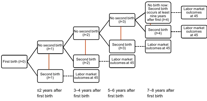
For the purpose of implementing the framework, it is convenient to think of time as discrete (Sianesi 2004); in my analysis, mothers who are eligible for a second birth (the treatment group) at timet are those who still have not had a second child after t years following the first birth, irrespective of what happens aftert. This is analogous to a survival model that includes duration-specific parameters. The comparison group for women who have a second birth at timet consists of all women who have experienced at leastt years after the first birth who have not yet experienced a second birth but will experience a second birth at some point in the future. Thus, the comparison of the effect of a second birth at timet on labor market outcomes is with women who have reachedt years after the first birth. For example, consider two women with first births occurring in 1980. Woman A has a second child in 1982, while Woman B has a second child in 1985. Att=1 (≤2-year interval), women with a second child born within two years of the first, such as Woman A, are compared to women whose first child was also born two years before but whose second child will not be born until more than two years after the first, such as Woman B. Figure 1 shows this comparison across the different time points in the analysis, from t=1 (≤2-year interval) tot=4 (7–8-year interval); the red lines identify the comparisons.13The main analysis includes five categories: 1–2
years (intervals up to and including 24 months); 3–4 years (birth intervals of 25 to 48 months); 5–6 years (birth intervals of 49 to 72 months); 7–8 years (birth intervals of
11 There are limitations with regard to estimating a causal effect that are discussed in this section and further
elaborated following the presentation of results. Nonetheless, the goal of the analysis is to achieve the best estimate of a causal effect, and the methods described in this section are designed for that purpose and implemented with that goal in mind.
12 Similar methods have been used in sociology previously (see, e.g., Sharkey and Elwert 2011; Wodtke,
Harding, and Elwert 2011).
13 One challenge with these models is that at longer intervals the comparison group potentially becomes more
73–96 months); and 9+ years (always a comparison category only; birth intervals of 97 or more months).
Figure 1: Second-birth states fromt=0 tot=9+ years after first birth
≤2 years after first birth
3–4 years after first birth
5–6 years after first birth
7–8 years after first birth
To identify the effect of a second birth at timet on labor market outcomes I use IPT weighting based on propensity scores, which is an alternative approach to propensity score matching. This method is useful – compared to OLS, for example – because it corrects for two sources of bias: differences in the supports of the variables and differences in the shapes of the distributions of variables in the region of common support (Heckman et al. 1998). In other words, the method increases the overlap in the values of variables for the two comparison groups (treatment and control groups), and it makes the shapes of these distributions of values more similar.
A third potential type of bias identified by Heckman et al. (1998) is selection bias. Obtaining the effects of second births at different intervals on women’s labor force outcomes requires making assumptions about selection (also true in an OLS framework, not only in a dynamic potential outcomes framework). In particular, it requires making the conditional independence assumption (CIA), which states that treatment status (i.e., having or not having a second birth) is random conditional on a set of X observed covariates (Rosenbaum and Rubin 1983; Rubin 1978). The variables in X cannot be affected by the treatment, andX must include all of the variables that affect both the treatment and the outcomes.
First birth (t=0)
No second birth (t=1)
No second birth (t=2)
No second birth (t=3)
No birth now: Second birth occurs at least
nine years after first (t=4)
Labor market outcomes
at 45
Second birth (t=4)
Labor market outcomes
at 45
Second birth
(t=3) outcomes at 45Labor market
Second birth
(t=2) outcomes at 45Labor market
Second birth
In this dynamic context, this means that at each period the second birth is random conditional on observed covariates prior to that period, that these observed covariates are not affected by the second birth, and that the observed covariates included in the estimation comprise all of the variables affecting both the second birth at that time and the labor market outcomes.14 It is not possible to test whether the CIA is valid without
conducting an experiment, but sensitivity analyses can help with assessment of validity.15 The variables in X are chosen based on theory and past research (Sianesi
2004). The dynamic CIA is plausible in this study because there is extensive data available longitudinally in the survey, and there is a large body of past research detailing the factors influencing timing of childbearing, previously described in Section 3.2.3, where I describe the included control variables.
3.3.1 Estimation
I estimate propensity scores and use them to create IPT weights, rather than matching on the propensity score directly (Busso, DiNardo, and McCrary 2014). To construct the IPT weights, I first estimate four logit models of selection into the different birth intervals and predict propensity scores. At the initial period of possible ‘treatment’ each woman is in the same treatment state – she has just had a first birth. This is followed by four two-year-long periods in which different treatment sequences could be realized (i.e., in each period a woman can have a second child or postpone a second child). Each logit model estimates the probability of a second birth in periodt, conditional onX and on having reached timet without having already had a second birth. This is analogous in many ways to a hazard model, in which the population at risk is changing over time, as some women experience second births and some will not experience a second birth until some point in the future. Recently, Fitzenberger, Sommerfeld, and Steffes (2013) used this approach to study time to first birth in Germany. I provide estimates of the coefficients from the propensity score models in Table A-2. Examining the pseudo-R2
values suggests that the models predict a second birth fairly well.
Once I have estimated the propensity scores for each period, I use the scores to generate IPT weights to be used in estimating the motherhood penalty. The most basic
14 Because there is a timing component involved (multiple years in which a second birth can occur), it is
necessary for the CIA to hold in terms of future second births (dynamic CIA or DCIA). As such, the CIA does not have to hold in the conventional sense: having a second birth vs. never having a second birth. Instead it must hold at the margin: having a second birth at timet vs. postponing the second birth to at leastt+1 (see, e.g., Sianesi 2004).
15 However, a formal sensitivity analysis along the lines of Robins (1999) requires assumptions about
form an IPT weight can take is 1/p wherep indicates the propensity score derived from the logit model. In practice, stabilized or normalized weights are more commonly used, to guard against weights that are arbitrarily large. Busso, DiNardo, and McCrary (2014) show that IPT weighting is a good method for this type of analysis, but only if the weights are normalized.16
After I normalize the weights I then calculate the average treatment effect of a second birth at each time t on a mother’s labor market outcomes to estimate the motherhood penalty (i.e., ATT). The main model is a simple regression of birth-at-time t on the labor force outcome, weighted by the IPT weight. Standard errors are calculated using Huber/White sandwich estimators to adjust for the two-stage estimation process. Finally, after obtaining the ATT for each time period, I follow the strategy of Abadie and Imbens (2011) and Fitzenberger, Sommerfeld, and Steffes (2013) and estimate ex post outcome regressions to examine effect heterogeneity. Specifically, I first add a control for age at first birth and separately a control for a college degree to test Hypothesis 2. I then add an interaction term to the simple regression on labor force outcomes, interacting birth-at-time t separately with age at first birth and then with education to test Hypothesis 3. I conduct Wald tests of the coefficients using the Bonferroni adjustment to address multiple comparisons in the pairwise tests. Rather than interacting the birth interval indicator with a continuous measure of age, I include age as a set of dummy variables to better account for possible nonlinearities in effects. There are three age indicators. The first indicates first births occurring between ages 18 and 29 (omitted category); the second indicates first births at ages less than 18; and the third indicates first births occurring at age 30 or older. I chose cutoffs of ages 18 and 30 because past research has indicated that childbearing before age 18 is distinct in a number of ways from childbearing at later ages and because in past literature a motherhood premium for postponement was found for women 30 and older at first birth (e.g., Amuedo-Dorantes and Kimmel 2005).
4. Results
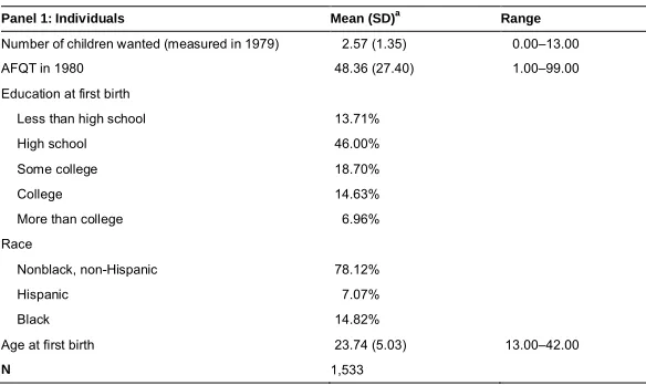
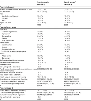
Table 1 presents the sample-weighted descriptive statistics for the analytic sample.17
There are a couple of features to note. First, the average age at first birth is about 23.7
16 Sensitivity analyses discussed in the Results section also included estimates using nearest neighbor
matching in line with Busso, DiNardo, and McCrary’s (2014) suggestion that researchers examine estimates using a variety of approaches.
17 Table A-1 presents descriptive statistics for the analytic sample and the overall sample of women before
years, which is consistent with the national average in the years in which most women in the sample had a first birth (1980–1989) (Hamilton and Martin 2013). Examination of the distribution of age at first birth in the sample (not shown) indicates that 25% of women had a first birth at age 19 or younger, while the oldest 25% of mothers in the sample had first births at age 26 or later. About 12% of first births occurred to women under the age of 18, while only about 1% of first births occurred to women over the age of 35. Thus, by measuring women’s outcomes at age 45, most women in the sample will have had ample time to return to work, following the birth of their second child. Indeed, at age 45 only 8% of the sample were not working in the labor force. Respondents who are working at age 45 have hourly wages averaging about $18. Over the life course, women in the sample have worked nearly 39,000 hours on average, and they have accumulated an average of about $415,000 in earnings. On average, by age 45 women in the sample have 2.6 children; an examination of the distribution indicates that a little over 50% of the sample have only two children by age 45, and the remaining women have three or more children, with the bulk of these women having three children.
Table 1: Sample-weighted descriptive statistics for the main analytic sample Panel 1: Individuals Mean (SD)a Range
Number of children wanted (measured in 1979) 2.57 (1.35) 0.00–13.00 AFQT in 1980 48.36 (27.40) 1.00–99.00 Education at first birth
Less than high school 13.71% High school 46.00% Some college 18.70% College 14.63% More than college 6.96% Race
Nonblack, non-Hispanic 78.12% Hispanic 7.07%
Black 14.82%
Age at first birth 23.74 (5.03) 13.00–42.00
N 1,533
Table 1: (Continued) Panel 2: Person-years
Marital status
Never married 24.92% Married 60.50% Separated/divorced 14.58% Occupation is professional/managerial 0.31 Sector
Private sector 78.05% Government 15.54% Self-employed/working without pay 6.42%
Tenure with employer (years) 4.26 (5.21) 0.02–37.87 Part-time worker 0.24
Not working in the labor force 0.20 Family economic resources
(household income minus respondent income) 36,766.54 (42,781.42) 0.00–252,740.20 Respondent resides in the South 0.34
Respondent lives in urban area 0.73
Hourly wage of respondent 12.22 (10.24) 0.00-49.07 Annual income of respondent 22,230.76 (21,948.26) 0.00–103,000.00 Cumulative hours of work experience 18,327.13 (15,976.87) 0.00–59,947.00 Cumulative earnings of respondent 202,352.50 (228,123.30) 0.00–2,042,437.00
N 36,103
Panel 3: At age 45
Hourly wage of respondent, if working 18.21 (10.99) 0.01–48.08 Cumulative earnings of respondent 415,025.70 (281,062.00) 0.00–1,836,467.00 Cumulative hours of work experience 38,642.29 (14,629.05) 0–59,947.00 Not working in the labor force 0.08
Total number of children 2.63 (0.96) 2–11
N 1,533
Note:aStandard deviations not provided for proportions, for which the entire distribution is provided.
Figure 2: Number of mothers by birth interval
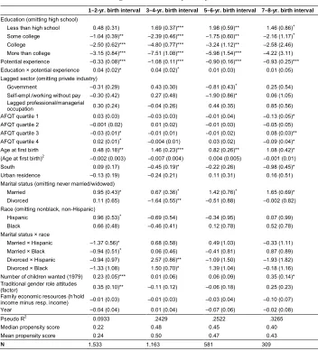
4.1 Predictors of birth spacing
The results for the logit models predicting different birth-spacing intervals are shown in Table A-2. A few key predictors stand out. Age at first birth is a positive predictor of a birth at all intervals. This is consistent with the idea that women who are older at a first birth will have less time available for subsequent births. Being married, as opposed to being never married, is a positive predictor of a second birth for all intervals. Having at least some college education is a negative predictor of birth intervals of six or fewer years, while having less than high school education is a positive predictor of all intervals except those shorter than two years. This is consistent with the possibility raised in the literature that college-educated women might try to minimize the career penalties they will incur by having a second child by spacing their children farther apart. Past research in the United States and Sweden has indeed found that such behavior would be beneficial for these women (Karimi 2014; Troske and Voicu 2013).
4.2 Birth spacing and labor market outcomes (Hypothesis 1)
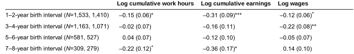
The results of the focal models of the role of birth spacing for women’s midlife labor market outcomes are shown in Table 2. Hypothesis 1 stated that the magnitude of the motherhood penalty for a second birth would decline as the birth interval increases. If the hypothesis were supported we would expect to see that the penalties would become smaller as we look down the columns at each successive birth interval. The results in Table 2 indicate that this may be true for some women, but the pattern is not monotonic. Women with birth intervals shorter than two years do appear to experience
370
582
272
136 173
significant penalties compared to mothers with longer birth intervals: 14%18 lower
cumulative work hours by age 45 (p<.05); 27% lower cumulative earnings by age 45 (p<.001); and 11% lower wages at age 45 (p<.10). By comparison, women with 3–4-and 5–6-year birth intervals do not appear to experience significant penalties compared to mothers with longer intervals, the exception being wages at age 45 for women with 3–4-year birth intervals. But significant penalties for cumulative outcomes return for women with 7–8-year birth intervals compared to women with the longest interval; these women have 20% fewer work hours and 30% lower cumulative earnings by age 45. Thus, the results for Hypothesis 1 are mixed. There is some evidence that longer intervals may be associated with smaller second-child penalties by midlife, but the pattern is not consistent across all of the intervals. This begs the question whether there may be unobserved heterogeneity at play. I return to this possibility of heterogeneity in Section 4.4.
Table 2: Inverse probability of treatment-weighted estimates of the average effect of a second birth on log cumulative work hours (in 1,000s), log cumulative earnings (in $10,000s), and log hourly wages, at age 45, by two-year birth intervals
Log cumulative work hours Log cumulative earnings Log wages 1–2-year birth interval (N=1,533, 1,410) –0.15 (0.06)* –0.31 (0.09)*** –0.12 (0.06)+
3–4-year birth interval (N=1,163, 1,071) –0.02 (0.07) –0.16 (0.11) –0.22 (0.08)** 5–6-year birth interval (N=581, 527) 0.04 (0.07) –0.12 (0.10) –0.05 (0.07) 7–8-year birth interval (N=309, 279) –0.22 (0.12)+ –0.36 (0.17)* 0.14 (0.10)
Notes:+ p<.10; * p<.05; ** p<.01; *** p<.001. Cumulative models include women not working at age 44 or 45. Robust standard errors,
clustered at the individual level, are estimated. Log wage model includes only women working at age 44 or 45, resulting in a smaller sample size.
4.3 Age at birth, human capital, and labor market outcomes (Hypothesis 2)
The results presented in Table 2 provide average effects of a second birth at each time intervalt for women with a second birth at timet, as opposed to postponing the second birth to a later time. The mixed results suggest there could be unobserved heterogeneity that needs examination. Before turning attention to this possible heterogeneity, I examine the evidence for Hypotheses 2a and 2b to determine whether age at first birth and education could plausibly act as moderating factors in this sample. Hypothesis 2a stated that women who postpone a first birth to at least age 30 would have smaller motherhood penalties than those who do not postpone to at least age 30. If this
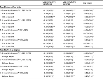
hypothesis is supported we should see smaller penalties for women age 30 and older at first birth compared to women who were younger at first birth. Evidence for Hypothesis 2a can be found in Panel 1 of Table 3. Looking at all three outcomes, the hypothesis is supported almost across the board. Only for log wages in the model of women with birth intervals of seven or more years is postponement not statistically significant. Exponentiating the coefficients on being age 30 or older at first birth, and averaging across models, indicate that, compared to women aged 18–29 at first birth, women who postpone achieve about 22% greater work hours by age 45; more than twice the cumulative earnings; and wages at age 45 that are roughly 25%–40% higher depending on the model. Thus, there is robust support for Hypothesis 2a that women who postpone a first birth have smaller penalties than those who do not postpone.
Table 3: Inverse probability of treatment-weighted estimates of the average effect of a second birth on log cumulative work hours (in 1,000s), log cumulative earnings (in $10,000s), and log hourly wages, at age 45, by two-year birth intervals, accounting for age at first birth (Panel 1) and college degree (Panel 2)
Log cumulative work hours
Log cumulative
earnings Log wages Panel 1: Age at first birth
1–2-year birth interval (N=1,533, 1,410) –0.15 (0.06)** –0.33 (0.08)*** –0.12 (0.06)+
<18 at first birth –0.09 (0.07) –0.45 (0.12)*** –0.10 (0.08) ≥30 at first birth 0.25 (0.05)*** 0.77 (0.08)*** 0.33 (0.09)*** 3–4-year birth interval (N=1,163, 1,071) –0.01 (0.06) –0.11 (0.10) –0.20 (0.08)*
<18 at first birth –0.16 (0.16) –0.43 (0.20)* –0.13 (0.08) ≥30 at first birth 0.20 (0.05)*** 0.71 (0.08)*** 0.25 (0.08)** 5–6-year birth interval (N=581, 527) 0.05 (0.07) –0.10 (0.10) –0.04 (0.07)
<18 at first birth –0.04 (0.08) –0.18 (0.12) –0.06 (0.08) ≥30 at first birth 0.20 (0.06)** 0.71 (0.11)*** 0.22 (0.09)* 7–8-year birth interval (N=309, 279) –0.21 (0.12)+ –0.33 (0.15)* 0.14 (0.10)
<18 at first birth –0.26 (0.21) –0.31 (0.27) –0.02 (0.13) ≥30 at first birth 0.24 (0.08)** 0.86 (0.10)*** 0.17 (0.12) Panel 2: College degree
1–2-year birth interval (N=1,533, 1,410) –0.15 (0.06)* –0.30 (0.09)** –0.11 (0.06)+
College degree 0.05 (0.14) 0.70 (0.18)*** 0.22 (0.12)+ 3–4-year birth interval (N=1,163, 1,071) –0.02 (0.07) –0.14 (0.10) –0.21 (0.08)**
College degree 0.26 (0.05)*** 0.88 (0.07)*** 0.24 (0.10)* 5–6-year birth interval (N=581, 527) 0.04 (0.08) –0.12 (0.10) –0.05 (0.07)
College degree 0.21 (0.06)** 0.74 (0.09)*** 0.10 (0.16) 7–8-year birth interval (N=309, 279) –0.23 (0.12)+ –0.39 (0.16)* 0.12 (0.10)
College degree 0.33 (0.11)** 0.85 (0.17)*** 0.48 (0.14)**
Notes:+p<.10; * p<.05; ** p<.01; *** p<.001. Cumulative models include women not working at age 44 or 45. Robust standard errors,
clustered at the individual level, are estimated. Log wage model includes only women working at age 44 or 45, resulting in a smaller sample size.
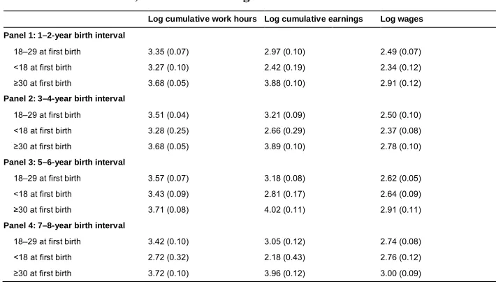
4.4 Heterogeneous effects by age at first birth and education (Hypothesis 3)
postponed a first birth to at least age 30 would have smaller penalties than those who did not postpone to at least age 30 (Hypothesis 3a). If this hypothesis is supported we should see nonsignificant differences with regard to postponement for the shortest birth interval but a growing importance of postponement and significant effects at longer intervals. To make the interpretation of the interactions more concrete, I provide estimated marginal means, rather than coefficients, in Table 4. Each panel of the table indicates the estimated marginal mean with a second birth at that interval, broken down by age at first birth. Note that these marginal means are still logged; to calculate actual mean cumulative work hours, for example, one would need to exponentiate the appropriate marginal mean value. As an example, for the 1–2-year birth interval and cumulative work hours, the estimated means are 28,503 for women aged 18–29 at first birth ((e^3.35)*1,000); 26,311 for women under age 18 at first birth; and 39,646 for women at least age 30 at first birth.
Table 4: Estimated marginal means derived from inverse probability of treatment-weighted estimates of the average effect of a second birth on log cumulative work hours (in 1,000s), log cumulative earnings (in $10,000s), and log hourly wages, at age 45, by two-year birth
intervals, interacted with age at first birth
Log cumulative work hours Log cumulative earnings Log wages Panel 1: 1–2-year birth interval
18–29 at first birth 3.35 (0.07) 2.97 (0.10) 2.49 (0.07) <18 at first birth 3.27 (0.10) 2.42 (0.19) 2.34 (0.12) ≥30 at first birth 3.68 (0.05) 3.88 (0.10) 2.91 (0.12) Panel 2: 3–4-year birth interval
18–29 at first birth 3.51 (0.04) 3.21 (0.09) 2.50 (0.10) <18 at first birth 3.28 (0.25) 2.66 (0.29) 2.37 (0.08) ≥30 at first birth 3.68 (0.05) 3.89 (0.10) 2.78 (0.10) Panel 3: 5–6-year birth interval
18–29 at first birth 3.57 (0.07) 3.18 (0.08) 2.62 (0.05) <18 at first birth 3.43 (0.09) 2.81 (0.17) 2.64 (0.09) ≥30 at first birth 3.71 (0.08) 4.02 (0.11) 2.91 (0.11) Panel 4: 7–8-year birth interval
18–29 at first birth 3.42 (0.10) 3.05 (0.12) 2.74 (0.08) <18 at first birth 2.72 (0.32) 2.18 (0.43) 2.76 (0.12) ≥30 at first birth 3.72 (0.10) 3.96 (0.12) 3.00 (0.09)
Looking first at cumulative work hours in Column 1, it appears that women who postponed a first birth to at least age 30 always have higher work hours, while women experiencing a first birth prior to age 18 have the lowest. An examination of the Wald test results indicate that at the 5–6-year (p<.05) and 7–8-year (p<.01) birth intervals only the comparison between mothers younger than age 18 at first birth and women who postponed the first birth to at least age 30 is statistically significant. Thus, for cumulative work hours, the hypothesis does not hold in general, but rather only in comparison to the most disadvantaged mothers.
Turning to cumulative earnings in Column 2, we see the same pattern, whereby mothers under age 18 at first birth have the lowest earnings, mothers aged 18–29 at first birth have higher earnings, and mothers at least age 30 at first birth have the highest earnings. In contrast to cumulative work hours, Wald test results indicate that women who postponed a first birth to at least age 30 always have significantly better outcomes than women who did not postpone a first birth to age 30 (p<.001 in most cases). This result is partially in conflict with Hypothesis 3a, since women who postponed a first birth and have shorter birth intervals are also seeing benefits, not only women with longer birth intervals, and the magnitudes of the differences between the postponers and nonpostponers are fairly stable across the intervals.
Turning finally to log wages in Column 3, in models of working women only, we see limited evidence for the hypothesis. According to the results of the Wald tests, women who postponed a first birth to at least age 30 have significantly higher wages than women with a first birth prior to age 18 in models of the 1–2-year (p<.01) and 3–4-year (p<.01) birth intervals. They have significantly higher wages than women aged 18–29 at first birth in the 1–2-year (p<.01) and 5–6-year (p<.05) models. But women who postponed a first birth to at least age 30 do not have higher wages at age 45 when they have longer birth intervals, which is inconsistent with Hypothesis 3a.
Overall, there is very good evidence that postponement of a first birth to at least age 30 has a positive effect on midlife labor market outcomes. There is less consistent evidence that it meaningfully modifies the effects of birth spacing on outcomes, though in the case of log wages, age at first birth modifies the effects of birth spacing at the shorter (and mid-length) intervals, but not at the 7–8-year birth interval as hypothesized.19
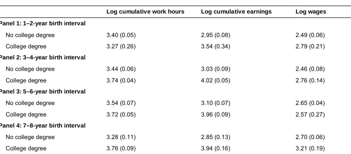
I also hypothesized that at longer birth intervals, women with college degrees would have smaller penalties than those without college degrees (Hypothesis 3b). If this hypothesis is supported we should see nonsignificant differences with regard to education for the shortest birth interval but growing importance of education and
19 As discussed in the Appendix, I examined whether these postponement effects are also seen when looking
significant effects at longer intervals. As with the results for Hypothesis 3a, I provide estimated marginal means, rather than coefficients, in Table 5 for ease of interpretation. Each panel of the table indicates the estimated marginal mean with a second birth at that interval, broken down by whether the respondent has a college degree. All marginal means are still logged as noted previously.
Table 5: Estimated marginal means derived from inverse probability of treatment-weighted estimates of the average effect of a second birth on log cumulative work hours (in 1,000s), log cumulative earnings (in $10,000s), and log hourly wages, at age 45, by two-year birth
intervals, interacted with college degree
Log cumulative work hours Log cumulative earnings Log wages Panel 1: 1–2-year birth interval
No college degree 3.40 (0.05) 2.95 (0.08) 2.49 (0.06) College degree 3.27 (0.26) 3.54 (0.34) 2.79 (0.21) Panel 2: 3–4-year birth interval
No college degree 3.44 (0.06) 3.03 (0.09) 2.46 (0.08) College degree 3.74 (0.04) 4.02 (0.05) 2.76 (0.14) Panel 3: 5–6-year birth interval
No college degree 3.54 (0.07) 3.10 (0.07) 2.65 (0.04) College degree 3.72 (0.05) 3.96 (0.09) 2.57 (0.27) Panel 4: 7–8-year birth interval
No college degree 3.28 (0.11) 2.85 (0.13) 2.70 (0.06) College degree 3.76 (0.09) 3.94 (0.16) 3.21 (0.19)
Notes: Estimated marginal means shown with delta-method standard errors.
Looking first at cumulative work hours in Column 1, it appears that women with a college degree have higher work hours than women without a college degree, except for women with a short birth interval. An examination of the Wald test results indicates that for all but the 1–2-year birth interval the differences between these groups are statistically significant (p<.001). Thus, for cumulative work hours, the hypothesis holds; college-educated women with short birth intervals do not have an advantage over women with the same birth interval and no college degree, but at the longer birth intervals having a college degree is advantageous.
p<.05 for 5–6 years; p<.01 for 7–8 years). Thus, the results for cumulative earnings also support the hypothesis: Women with short intervals have similar outcomes regardless of education, whereas at longer birth intervals the college-educated women are advantaged.
Turning finally to log wages in Column 3, in models of working women only, we see limited evidence for the hypothesis. Looking at the estimated marginal means descriptively, we can see that college-educated women still appear to be advantaged at most birth intervals, but except for the 7–8-year birth interval the Wald test results indicate that these are not statistically significant differences. For the 7–8-year birth interval college-educated women have statistically significantly higher log wages at age 45 than those without a college degree (p<.05). Thus, the results for log wages also support the hypothesis, though it is only at the 7–8-year birth interval where the interaction between spacing and a college education is significant.
Overall, there is very good evidence that having a college degree has a positive effect on midlife labor market outcomes, and there is consistent evidence that it meaningfully modifies the effects of birth spacing on outcomes. For women with the shortest birth intervals, postponement of a first birth to at least age 30 helped to reduce the midlife penalties of having a second child, but having a college degree does not. On the other hand, at longer intervals having a college degree reduces penalties more consistently than postponement of a first birth. These results suggest that postponement and education work differently to attenuate the motherhood penalty.
4.5 Description of supplemental analyses
5. Discussion
In this study I set out to examine whether different birth-spacing patterns were associated with the accumulation of motherhood penalties in the labor market at midlife for US women. While spacing is mentioned in the early economic research linking childbearing and labor force participation for mothers, it has been understudied. Informed by these early theories and contemporary research, I tested three hypotheses. Hypothesis 1 states that the magnitude of the motherhood penalty for a second birth will decline as the birth interval increases. The results of models testing Hypothesis 1 provide evidence of a U-shape rather than a linear decline. For cumulative work hours and cumulative earnings, women with the 1–2-year and 7–8-year birth intervals have the largest penalties. For log wages, women with birth intervals of 1–2 and 3–4 years have larger penalties than women with longer birth intervals. Thus, Hypothesis 1 was not supported for cumulative outcomes but is somewhat supported for log wages.
Having established that the postponement and education patterns seen in past literature persist for midlife outcomes, I next tested Hypothesis 3 to assess heterogeneity in motherhood penalties related to birth spacing. Hypothesis 3a states that at longer birth intervals women who postponed a first birth to at least age 30 will have smaller penalties than those who did not postpone to at least age 30. Hypothesis 3b states that at longer birth intervals women with college degrees will have smaller penalties than those without college degrees. The evidence for Hypothesis 3 is mixed. With regard to postponement, although there is good evidence that postponement of a first birth to at least age 30 has positive effects on midlife labor market outcomes, as noted in the discussion of Hypothesis 2, there is little evidence that it modifies the effect of birth spacing on outcomes in the way hypothesized. Postponement does help to reduce midlife labor market penalties of having a second child, but this appears to be true for women with shorter birth intervals more than for women with longer birth intervals. In this way, rather than amplifying the possible human capital benefits of a longer birth interval, postponement seems to help protect women with shorter birth intervals that might otherwise be disadvantageous. This contrasts with Karimi’s (2014) findings for Sweden. But there is evidence consistent with Hypothesis 3 for education. Education has a positive effect on midlife labor market outcomes, and at longer birth intervals having a college degree reduces penalties more consistently than postponement of a first birth. For Sweden, Karimi (2014) found similar interactive results – longer birth intervals were especially beneficial for women with higher education.
There are limitations to the analysis, including those related to causal inference. The dynamic IPT weighting method simulates random assignment, but second births are still not randomly assigned to occur at different intervals. This is a limitation of the literature more generally, as one cannot assign women to give birth at particular times. Researchers have sometimes tried to address the nonrandomness of births using instrumental variable methods – for example, instrumenting using miscarriages – but these methods also have important limitations (Wilde, Batchelder, and Ellwood 2010). Furthermore, there is no common wisdom about which spacing intervals are better. Indeed, the literature suggests this may differ for different types of women. As such, instrumental variables would not obviously improve upon the IPT-weighted estimates. However, we cannot abandon the search for causal estimates because of these limitations. Rather, we must employ the best methods we have for causal inference and examine the sensitivity of results to different specifications. I have done this in the sensitivity analyses described in the Appendix, but in the case of observational data it is impossible to prove that the dynamic CIA always holds.
restrictions is quite modest for estimating the effects of a second birth occurring at several possible time points and allowing for heterogeneity by age at first birth and education. Because of this limitation, the coefficients may be imprecisely estimated, in some cases masking what would otherwise be statistically significant results. Nevertheless, the main results are quite consistent across specifications.
Finally, there are limitations in terms of the variables available with which to predict a second birth. A number of other variables could influence the timing of a second birth, such as negotiations between partners, unobserved changes in job-related duties, and the “quality” of the first child. That is to say, if the first child is difficult to parent or is frequently ill mothers may delay having a second child, while if the first child is easy to parent mothers might decide to have a second child sooner than they had originally anticipated. If future researchers can leverage such variables, they may gain additional insight into the determinants of birth spacing. Additionally, “unexpected” or “unintended” birth intervals – arising, for example, from a mistimed pregnancy – may have different consequences for women’s economic outcomes than intended or planned birth intervals, and in this paper I cannot address that possibility. As such, I focused primarily on determining the individual economic consequences of different birth intervals regardless of the underlying mechanisms. Thus, this study serves as a first step in examining the underexplored nature of the relationship between birth spacing and women’s labor market outcomes