Volume 38 - Article 29 | Pages 773–842

(1)

VOLUME 38, ARTICLE 29, PAGES 773

,

842 PUBLISHED 1 MARCH 2018

http://www.demographic-research.org/Volumes/Vol38/29/ DOI: 10.4054/DemRes.2018.38.29

Research Article

Gompertz, Makeham, and Siler models explain

Taylor’s law in human mortality data

Joel E. Cohen

Christina Bohk-Ewald

Roland Rau

This open-access work is published under the terms of the Creative Commons Attribution 3.0 Germany (CC BY 3.0 DE), which permits use, reproduction, and distribution in any medium, provided the original author(s) and source are given credit.

(2)

1 Introduction 774

2 Data and methods 776

2.1 Three theoretical models of mortality 776 2.2 Taylor’s law, mean and variance of mortality 777 2.3 Statistical methods and visualization 778

2.3.1 Parameter estimation 778

2.3.2 Analysis of log–log linearity 778

2.3.3 Visualizing the age profile of TL 778

2.3.4 Analysis of covariance 779

2.4 Availability of data and supplementary information 780

3 Results 780

3.1 Fitted mortality of Gompertz, Makeham, and Siler models 780 3.2 Statistical and visual tests of TL in observed and fitted mortality 783 3.2.1 Log-log linearity and r2_values ₇₈₃

3.2.2 Visually comparing age profiles between observed and modeled mortality

792

3.2.3 Slopes of TL 793

3.3 Mathematical proof and theoretical explanations for TL in Gompertz mortality

798

3.3.1 Gompertz mortality predicts TL with slope 2 under certain conditions

798

3.3.2 Temporal trend of βt alters the slope of TL fitted to Gompertz

mortality

798

3.3.2.1 Theoretical analysis 799

3.3.2.2 Numerical experiment 800

4 Conclusion 808

4.1 Summary 808

4.2 Future research 810

5 Acknowledgments 812

References 813

(3)

http://www.demographic-research.org 773

Gompertz, Makeham, and Siler models explain Taylor’s law

in human mortality data

Joel E. Cohen1

Christina Bohk-Ewald2 Roland Rau3

Abstract

BACKGROUND

Taylor’s law (TL) states a linear relationship on logarithmic scales between the variance and the mean of a nonnegative quantity. TL has been observed in spatiotemporal contexts for the population density of hundreds of species including humans. TL also describes temporal variation in human mortality in developed countries, but no explanation has been proposed.

OBJECTIVE

To understand why and to what extent TL describes temporal variation in human mortality, we examine whether the mortality models of Gompertz, Makeham, and Siler are consistent with TL. We also examine how strongly TL differs between observed and modeled mortality, between women and men, and among countries.

METHOD

We analyze how well each mortality model explains TL fitted to observed occurrence– exposure death rates by comparing three features: the log–log linearity of the temporal variance as a function of the temporal mean, the age profile, and the slope of TL. We support some empirical findings from the Human Mortality Database with mathematical proofs.

RESULTS

TL describes modeled mortality better than observed mortality and describes Gompertz mortality best. The age profile of TL is closest between observed and Siler mortality. The slope of TL is closest between observed and Makeham mortality. The Gompertz

1_{Laboratory of Populations, The Rockefeller University and Columbia University, New York, USA; Earth} Institute and Department of Statistics, Columbia University, New York, USA; Department of Statistics, University of Chicago, USA. Email:[email protected].

(4)

model predicts TL with a slope of exactly 2 if the modal age at death increases linearly with time and the parameter that specifies the growth rate of mortality with age is constant in time. Observed mortality obeys TL with a slope generally less than 2. An explanation is that, when the parameters of the Gompertz model are estimated from observed mortality year by year, both the modal age at death and the growth rate of mortality with age change over time.

CONCLUSIONS

TL describes human mortality well in developed countries because their mortality schedules are approximated well by classical mortality models, which we have shown to obey TL.

CONTRIBUTION

We provide the first theoretical linkage between three classical demographic models of mortality and TL.

1. Introduction

(5)

As an empirical generalization, TL invites attempts at explanation. Why is there an approximately linear relationship between the log of the temporal mean and the log of the temporal variance of mortality in many developed countries? Is this empirical regularity in human mortality just a coincidence, or does it come from an underlying pattern or mechanism? Here we answer these questions by comparing the completely empirical results of Bohk, Rau, and Cohen (2015) with the results of fitting three human mortality models: those of Gompertz (1825), Makeham (1860), and Siler (1979, 1983), which belong to the same family. We show that fitted mortality of these models obeys TL, exactly or approximately. Hence these models provide a theoretical basis for TL in human mortality.

Mortality models express mathematically the age schedule of mortality (that is, mortality as a function of age) in a given year. Models differ in the number of parameters they use and in the age ranges for which they model mortality well. The more parameters they use, the more flexibly they can fit mortality at different ages, but the more difficult they are to analyze mathematically. Gompertz’s model (1825), with two parameters, is one of the most popular models in demography. It assumes a linear increase in the logarithm of mortality with age. It usually describes well mortality at ages 30 to 90 (so-called senescent mortality). The model of Makeham (1860) adds to Gompertz’s model an additional age-independent constant to represent nonsenescent background mortality effective at all ages. This improves the fit at some younger ages. The model of Siler (1979, 1983) adds to the Makeham model an exponential decay in mortality to represent the decline in mortality from infancy to childhood. We discuss still more complicated mortality models in the concluding section 4.2 on future research.

The main objectives of this study are to examine whether the models of Gompertz, Makeham, and Siler are consistent with TL and can help to explain why and to what extent TL holds. In addition, we examine how strongly TL differs between observed mortality and model mortality schedules, between women and men, and among countries.

(6)

estimated from observed mortality year by year, both the modal age at death and the growth rate of mortality with age change over time.

Our analyses yield theoretical and empirical insights into the occurrence of TL in human mortality, giving a comprehensive picture of the extent to which TL describes the temporal variance in age-specific mortality in human populations. As we have confirmed TL to be a regular pattern (rather than a coincidence) in human mortality, it can be validly applied in other demographic studies such as generating and evaluating mortality forecasts.

In the remainder of this article, Section 2 describes data and methods; Section 3 presents results; and Section 4 summarizes the main findings. Appendices 1 and 2 give theorems, mathematical proofs, and approximations of TL for the Gompertz and Makeham models respectively. Supplementary material (online) includes estimates of model parameters, figures, and descriptive files.

2. Data and methods

We extracted deaths and life-years of exposures to the risk of death by single year of age, 0 to 100, and calendar year, 1960 to 2009, for 12 countries of the Human Mortality Database (2015). Given this data, we estimated observed mortality (or ‘observations’) defined as deaths divided by exposures by single years of age and calculated predicted mortality for each year separately with the models of Gompertz, Makeham, and Siler. Henceforth the word ‘observations’ means ‘occurrence–exposure death rates’.

2.1 Three theoretical models of mortality

We used mathematical expressions of the models of Gompertz, Makeham, and Siler that are based on the (old age) modal age at death (Horiuchi et al. 2013; Missov et al. 2015; Bergeron-Boucher, Ebeling, and Canudas-Romo 2015). The modal age at death is the age (beyond infancy and childhood) at which the probability density of life table deaths has a maximum. The conventional formulas for the models of Gompertz and Makeham use a parameter for an initial level of mortality instead of the modal age at death. The formulas based on the modal age at death, given below, are numerically more stable, have a better demographic interpretation, and are more comparable across populations and points of time (Horiuchi et al. 2013; Missov et al. 2015).

The Gompertz model expresses mortalityμ at agex in yeart as

(7)

Hereβtis the growth rate of mortality with age,Mt the modal age at death in yeart,

T the number of years of observations, and X the maximum observed age. The Gompertz model predicts, on a logarithmic scale of mortality and a linear scale of age, a linear increase in mortality from some young age to the oldest ageX = 100 here.

The Makeham model expresses mortalityμ at agex in yeart as

, = + ( ), > 0. (2)

The parameter βt is the same as in the Gompertz model. Makeham added ct to represent background mortality in year t, assumed to be the same at all ages x. The Makeham model predicts slowly increasing mortality from infancy through childhood to young adulthood; thereafter, it models a nearly linear increase in log mortality with increasing age.

The Siler model expresses mortalityμ at agex in yeart as

, = , + + , ,( ), > 0, , > 0. (3)

Here _, = of the Makeham and Gompertz models. Siler adds two additional parameters:αt is infant mortality, andβ1,t is the rate of decline with increasing agex of

childhood mortality in year t. The Siler model predicts decreasing mortality from infancy to childhood, slowly increasing mortality from childhood to young adulthood, and nearly linearly increasing log mortality with increasing age throughout adulthood.

2.2 Taylor’s law, mean and variance of mortality

A temporal TL describes a linear relationship of log10 of temporal variance (variance

over time) to log10 of temporal mean (mean over time) of mortalityμ at agex:

( ) = + ⋅ ( ), (4)

wherea is the intercept andb is the slope. With T years of observations or theoretical (fitted) values of mortality, the temporal mean of mortalityμ at agex is

( ) = ∑ ,, (5)

(8)

( ) = ∑ , − ( ) . (6)

We plot (on log–log coordinates) temporal variances and means of mortality for each age x in one national population at a time, separately for different national populations. These plots depict so-called cross-age-scenarios of TL (Bohk, Rau, and Cohen 2015).

2.3 Statistical methods and visualization 2.3.1 Parameter estimation

We estimated the values of the parameters of the models of Gompertz, Makeham, and Siler from deaths and exposures using the method of maximum likelihood. Specifically, we maximized a Poisson log-likelihood in R (2015) with the function DEoptim (Mullen et al. 2011).

2.3.2 Analysis of log–log linearity

To analyze how closely TL approximates the log temporal mean and log temporal variance of observed and/or modeled mortality, we used the linear correlation coefficient r2_{. The closer} _r2_{is to one, the better TL describes the relation of log}

temporal variance to log temporal mean of mortality.

2.3.3 Visualizing the age profile of TL

To compare the age profiles between observed and modeled mortality, we plotted the log10temporal variance of mortality as a function of the log10temporal mean by

(9)

2.3.4 Analysis of covariance

To analyze how well a theoretical model predicts the slope of TL fitted to observed mortality, we used the analysis of covariance.

1. To determine whether the slopes of TL differ between observed and modeled mortality (by sex, country, and model), we estimated a linear regression with an interaction term between the variables log10E(μx) and a dichotomous variable

model(with values ‘observed’ and ‘model’) using the lm()function in R:

( ) = + ( ) + + ( ( ) × ). (7)

We use observed mortality as the reference level for the categorical variable

model. The null hypothesis was that = 0, that is, that there was no difference

between the model and the observations in the slope of ( ) as a linear function of ( ). A very low p-value indicated that the coefficient of the interaction term is non-zero, and that the slope of TL of a model life table is not equal to the slope of TL of observed mortality data.

2a. We also used analysis of covariance to determine whether the slopes of TL differ between males and females (by country and mortality model). To analyze if the slopes of TL differed between males and females, we estimated a linear regression with an interaction term between the variables log10E(μx) and a dichotomous

variablesex (with values ‘male’ and ‘female’):

( ) = + ( ) + + ( ( ) × ). (8)

We used female mortality as the reference level. For the null hypothesis that

= 0, a very low p-value indicated that the coefficient of the interaction term is non-zero, and that the slope of TL is different between males and females.

2b. To analyze if sex differences in the slope of TL differ between observed and modeled mortality (by country and model), we estimated a linear regression with pairwise and three-way interaction terms among the variableslog10E(μx), sex,and

model. Here, unlike equation (7) above, the variable model had four values: 0 (observed), 1 (Gompertz), 2 (Makeham), 3 (Siler):

( ) = + ( ) + +

+ ( ( ) × ) + ( ( ) × ) + ( × )

(10)

Observed mortality was the reference level for model, as in equation (7), and female mortality was the reference level for sex. The null hypothesis was thatf = 0, that is, that model had no influence on the interaction betweensex and ( ).

2.4 Availability of data and supplementary information

In addition to the data on mortality, which is publicly available from the Human Mortality Database (2015), supplementary information deposited with this paper includes a spreadsheet (TLinMortalityModels.csv) with the values of 41 variables and a text file (TLinMortalityModels-Documentation-Variables.txt) that defines these variables. The spreadsheet gives the parameter estimates of the models of Gompertz, Makeham, and Siler for observed female and male mortality from 1960 to 2009 in 12 countries of the Human Mortality Database (2015). This information is graphed in Figures 1–17 and supplementary figures A-1–A-20. R code is available at:

https://github.com/christina-bohk-ewald/taylor-law-mortality.

3. Results

3.1 Fitted mortality of Gompertz, Makeham, and Siler models

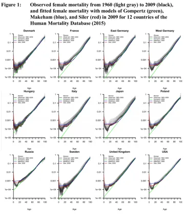
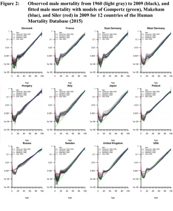
Before we analyze how consistent the models of Gompertz, Makeham, and Siler are with TL, we first show how well they fit observed mortality. Figures 1 and 2 display the observed age-specific mortality (on a logarithmic scale) as a function of age from 0 to 100, for women and men, respectively, from 1960 (light gray) to 2009 (black) in 12 countries of the Human Mortality Database (2015). Fitted mortality is depicted in green, blue, and red for the models of Gompertz, Makeham, and Siler, respectively, in 2009 for each country.

(11)

(12)

(13)

The Gompertz model fits observed mortality better at adult and older ages than at younger ages, where the predicted mortality is systematically and substantially too low. The Makeham model fits better than the Gompertz model, particularly for younger ages, but the modeled mortality increases monotonically with age, unlike the observations. The Siler model fits the age profile of mortality better than the Gompertz and Makeham models. None of the models reproduces the observed ‘accident bump’ of excess mortality of young adult ages. The findings in this paragraph confirm prior observations by others about the fit between human mortality data and the Gompertz, Makeham, and Siler models (e.g., Bongaarts 2005; Canudas-Romo 2008; Horiuchi et al. 2013; Bergeron-Boucher, Ebeling, and Canudas-Romo 2015).

3.2 Statistical and visual tests of TL in observed and fitted mortality

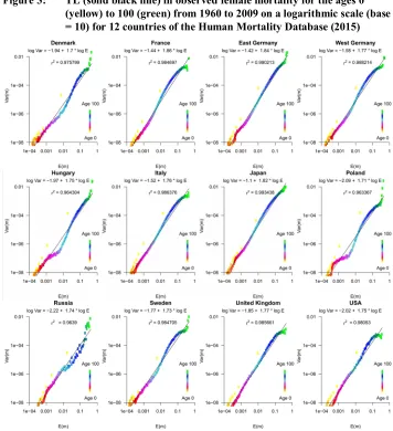
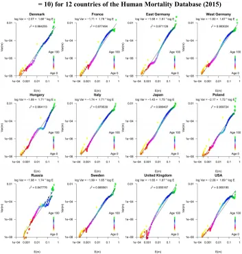
This section reports the statistical analysis and visual tests proposed in Section 2. Figures 3–10 display the cross-age-scenarios of TL for observed and fitted mortality of women and men, respectively, in 12 countries of the Human Mortality Database (2015). Odd-numbered figures are for females, even-numbered for males.

3.2.1 Log-log linearity andr2_values

Figures 3–4 compare the temporal means and temporal variances of observed mortality with TL (the fitted least squares straight line), on log–log coordinates. In these figures,

r2_{measures the linearity of observed log temporal variance as a function of observed}

log temporal mean. In Figures 5–10, r2_{measures the linearity of the log temporal}

variance of modeled mortality as a function of the log temporal mean of modeled mortality.

TL describes well the observed mortality (Figures 3, 4) and the mortality of the models of Gompertz (Figures 5, 6), Makeham (Figures 7, 8), and Siler (Figures 9, 10). For observations of women, 0.96 ≤ r2_{≤ 0.99, and of men, 0.95 ≤} _r2_{≤ 0.99, in the}

selected countries. Where the mortality models hadr2_{≥ 0.999, sometimes there was}

(14)

Figure 3: TL (solid black line) in observed female mortality for the ages 0 (yellow) to 100 (green) from 1960 to 2009 on a logarithmic scale (base = 10) for 12 countries of the Human Mortality Database (2015)

(15)

Figure 4: TL (solid black line) in observed male mortality for the ages 0 (yellow) to 100 (green) from 1960 to 2009 on a logarithmic scale (base = 10) for 12 countries of the Human Mortality Database (2015)

(16)

(17)

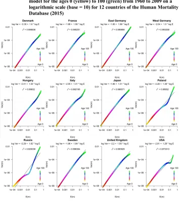
Figure 6: TL (solid black line) in fitted male mortality of the Gompertz model for the ages 0 (yellow) to 100 (green) from 1960 to 2009 on a

(18)

(19)

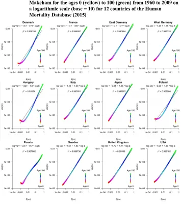
Figure 8: TL (solid black line) in fitted male mortality of the model of

(20)

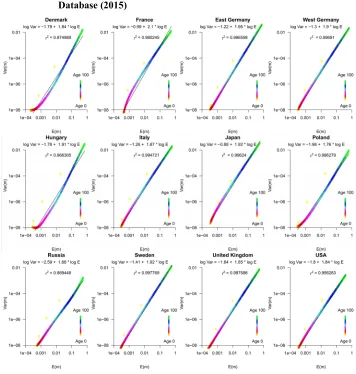
Figure 9: TL (solid black line) in fitted female mortality of the model of Siler for the ages 0 (yellow) to 100 (green) from 1960 to 2009 on a

(21)

(22)

According to the r2_{values, TL describes Gompertz mortality best among these}

three models. Appendix 1 gives a mathematical proof that TL describes Gompertz mortality exactly if the modal age at deathMtincreases linearly in time and if the rate of growth of mortality with ageβt is constant in time. The first assumption is close to reality, as we shall see. The second assumption is not:βt increased slightly over time within a narrow range, even thoughβt is hypothesized to be constant across individuals and over time (Vaupel 2010). Nevertheless, the excellent agreement between TL and Gompertz mortality is at least partially explained by this mathematical analysis.

3.2.2 Visually comparing age profiles between observed and modeled mortality

In this section, we visually compare the age pattern of TL between observed and modeled mortality.

TL in observed mortality data (Figures 3–4) has a typical pattern that is similar for women and men in many populations. Both the log10 temporal variance and the log10

temporal mean of mortality increase linearly from young adulthood (red) to the elderly (green), and they decrease from infancy (yellow) to childhood (orange). The changes in the log10 temporal mean are expected from the increasing mortality with age at older

ages and the decreasing mortality with age from infancy to childhood. The corresponding linear changes in the log10 temporal variance were not known prior to the

work of Bohk, Rau, and Cohen (2015).

TL of Gompertz mortality (Figures 5–6) mirrors the pattern of TL of the observations well at adult and old ages. However, both the log10 temporal variance and

the log10 temporal mean of mortality of infants and children (yellow to orange) are

modeled to be smaller than those of young adults (red), unlike the observations. This major difference between observed mortality and the Gompertz model arises because the Gompertz model assumes a log-linear increase in mortality from the youngest to the oldest age. The Gompertz model captures neither declining mortality from infancy to childhood nor its related effect on TL.

TL of Makeham mortality (Figures 7–8) mirrors the pattern of TL of the observations well at adult and old ages. However, both the log10 temporal variance and

the log10 temporal mean of mortality are modeled to be almost equal for infants and

(23)

childhood nor its related effect on TL. As expected, TL of Makeham mortality is closer than TL of Gompertz mortality to TL of observations.

TL of Siler mortality (Figures 9–10) mirrors reasonably well the pattern of TL of the observations for all ages in most of the 12 countries. The term in the Siler model that models declining mortality from infancy to childhood captures the related effect on TL.

From visually comparing the age profiles, we conclude that the TL of the Siler model (fitted to observed mortality) is closest to the TL of observed mortality.

3.2.3 Slopes of TL

In this section, we compare the slopes of TL between observed and modeled mortality.

A. Visual overview

Figure 11 displays the slope of TL for women on the horizontal axis and the slope of TL for men on the vertical axis for 12 countries of the Human Mortality Database (2015). Slopes are estimated from observed mortality (black) and from the fitted models of Gompertz (green), Makeham (blue), and Siler (red). Figure 11 summarizes 96 slopes (96 = 12 × 4 × 2). Only two slopes exceed 2 (for TL fitted to the Gompertz model for Russian males,b = 2.02; and for TL fitted to the Siler model for French females, b = 2.1). We regard these two slopes as outliers. All slopes exceed 1.

Slopes of TL estimated from observed mortality are closer to slopes estimated from the Makeham model than they are to the slopes estimated from the other two models. Women and men have greater slopes according to the Siler model than are estimated from observed mortality. Hence the Siler model assumes more rapid increases in the variance of mortality with increasing mean mortality than is observed. Women and men have substantially smaller slopes according to the Gompertz model than are estimated from observed mortality. The Gompertz model assumes slower increases in the variance of mortality with increasing mean mortality than is observed.

(24)

Figure 11: Scatterplot of slope of TL for women (horizontal axis) and men (vertical axis) for 12 countries of the Human Mortality Database (2015)

(25)

B. Covariance analysis

We examine differences in the slopes of TL between sexes and models using covariance analysis.

B1. Does the slope of TL for observed mortality differ from the slopes of TL for models?

The p-values of the test for the significance of the interaction termc3 in the analysis of

covariance, eq. (7), are given by sex, country, and model (Gompertz, Makeham, Siler) in Table 1.This analysis confirms the findings from Figure 11. Specifically, the slope of TL of the Makeham model is not significantly different from the slope of TL of observed mortality for women and men in almost all of the 12 countries. By contrast, the slope of TL of the Siler model is significantly different from the slope of TL of observed mortality for women and men in almost all 12 countries. An exception is, for example, Poland. The slope of TL of the Gompertz model is significantly different from the slope of TL of observed mortality for women and men in almost all 12 countries.

Table 1: P-values to test the null hypothesis of no differences in TL slope between observed data and the fitted models of Gompertz, Makeham, and Siler, for women and men in 12 countries of the Human Mortality Database (2015)

Equal to TL of observed data?

Gompertz Makeham Siler

Women Men Both Women Men Both Women Men Both

All countries 0 0 0 0.073200 0.284200 0.032000 0 0 0

Denmark 0.005358 0 0 0.022461 0.231000 0.284805 0.000312 0.208000 0.000392

France 0 0 0 0.748900 0.076500 0.486783 0 0 0

East Germany 0 0.000006 0 0.000580 0.329880 0.011300 0 0.000120 0

West Germany 0 0 0 0.351730 0.986726 0.432000 0 0.000014 0

Hungary 0.000007 0.001720 0.005730 0.296356 0.078070 0.106000 0.000661 0.008880 0.000077

Italy 0 0 0 0.003660 0.000132 0.000004 0.000001 0.001448 0

Japan 0 0 0 0.035169 0.001420 0.001870 0 0 0

Poland 0 0.032000 0 0.021900 0.811000 0.141000 0.233800 0.177000 0.153

Russia 0.009401 0 0.789410 0.000337 0.028860 0.002170 0.213779 0.000048 0.01896

Sweden 0 0 0 0.000002 0.532277 0.001853 0 0.000214 0

United Kingdom 0 0 0 0.002140 0.009960 0.000722 0.000380 0.000650 0.000003

United States 0 0 0 0.051616 0.114000 0.970258 0.000395 0 0

(26)

B2a. Does the slope of TL differ between males and females for observed mortality and for models?

The p-values of the test for the significance of the interaction term d3 in eq. (8) are

given by country for observed mortality and models in Table 2.

Table 2: P-values to test the null hypothesis of no differences between females and males in the slope of TL fitted to observed death rates and in the slope of TL fitted to the models of Gompertz, Makeham, and Siler, in 12 countries of the Human Mortality Database (2015)

Sex differences in TL? Observed data Gompertz Makeham Siler

All countries 0.023190 0.087000 0.199000 0.000290

Denmark 0.644000 0 0.000844 0.000736

France 0.031800 0.204590 0.069400 0.000017

East Germany 0.306800 0.187000 0.943370 0.510000

West Germany 0.000968 0.336000 0.000136 0

Hungary 0.426000 0 0.920000 0.106000

Italy 0.126570 0.582600 0.000200 0.000514

Japan 0.003760 0 0.068200 0.000128

Poland 0.827000 0.000021 0.068100 0.335000

Russia 0.936100 0 0.095200 0.000035

Sweden 0.005600 0 0 0

United Kingdom 0.042600 0.000009 0 0

United States 0.171000 0 0.001040 0.001610

Note: A p-value below 0.001 indicates that the coefficient of the interaction term is statistically significantly non-zero. An entry of 0 means that the rounded value of p is 0.000000.

Slopes of TL fitted to observed mortality are not significantly different between males and females in almost all 12 countries. Withp = 0.001, West Germany is the only exception. However, the slopes of TL differ between males and females almost as strongly in countries like France, the United Kingdom, Japan, and Sweden. The vertical deviations from the diagonal in Figure 11 are similar for these four countries.

The slopes of TL of modeled mortality differ significantly between males and females for many countries. These sex differences are slightly more pronounced in the models of Gompertz and Siler than in the Makeham model. This supports the finding from Figure 11.

(27)

B2b. Do the sex differences in the slope of TL differ between observed mortality and models?

Table 3 lists the p-values of the test for the significance of the coefficientf7of the

three-way interaction among log10E(μx), sex, and model of eq. (9). Consistent with the

findings from Figure 11 and Table 2, the sex differences in the slope of TL do not differ much between the observed mortality and the models of Gompertz, Makeham, and Siler. Specifically, the sex differences in the slope of TL are not significantly different between observed mortality and the Makeham model in each of the 12 countries. The sex differences in the slope of TL differ significantly between observed mortality and the Gompertz model in only three countries: Hungary, Russia, and the United States; and, though less significantly, in Sweden, Japan, West Germany, France, and Denmark. The sex differences in the slope of TL differ significantly between observed mortality and the Siler model in only two countries: Sweden and the United States; and, though less significantly, in Russia, France, and Denmark.

Table 3: P-values to test the null hypothesis of no differences in the sex differences in TL slope between observed mortality rates and fitted models of Gompertz, Makeham, and Siler, in 12 countries of the Human Mortality Database (2015)

Sex differences in TL of models equal to sex differences in

observed data? Gompertz Makeham Siler

All countries 0.005060 0.581010 0.349870

Denmark 0.025680 0.011860 0.045340

France 0.008070 0.164250 0.056650

East Germany 0.447548 0.392768 0.586554

West Germany 0.003030 0.527880 0.237640

Hungary 0 0.648766 0.515661

Italy 0.226781 0.329177 0.414148

Japan 0.029082 0.165447 0.817667

Poland 0.00917 0.128900 0.650510

Russia 0 0.303197 0.046573

Sweden 0.004344 0.006243 0.000250

United Kingdom 0.401217 0.643469 0.354857

United States 0.000003 0.013959 0.000247

Note: A p-value below 0.001 indicates that the coefficient of the interaction term is non-zero. An entry of 0 means that the rounded value of p is 0.000000.

(28)

countries in the 1980s and 1990s. By contrast, other European countries experienced a decline in the female–male differences in mortality (Oksuzyan et al. 2008).

3.3 Mathematical proof and theoretical explanations for TL in Gompertz mortality

In this section, we prove mathematically that the Gompertz model can explain the form of TL under certain conditions. We investigate theoretically whether the Gompertz model can explain the observed parameter values of TL.

3.3.1 Gompertz mortality predicts TL with slope 2 under certain conditions

We prove mathematically (in Appendix 1) that the Gompertz model eq. (1) with modal age at death increasing linearly in time and = > 0 obeys a cross-age-scenario of TL exactly with slopeb = 2. Appendix 1 gives an explicit form for the intercept of TL and a detailed proof. This theorem gives analytically the exact relation between the parameters of the Gompertz model and the parameters of TL in one simple case.

3.3.2 Temporal trend of alters the slope of TL fitted to Gompertz mortality

The theorem’s assumptions thatβt is constant over time and that the modal age at death

Mt increases linearly with time t cannot describe the reality of many countries since, empirically, the slopeb of TL fitted to the temporal mean and the temporal variance of observed mortality was always less than 2 (Figures 3–4), ranging from 1.65 to 1.87.

The numerical estimates of the parameters of all three mortality models, separately for females and males, for all countries and years, along with the parameters of linear regressions of these parameters as functions of time, are given in the Supplementary spreadsheet and graphed in Supplementary Figures A-1–A-20.

(29)

3.3.2.1 Theoretical analysis

We now analyze the impact of a temporal trend in on the estimated slope b of a cross-age-scenario of TL fitted to Gompertz mortality rates. In the Gompertz model eq. (1), appears twice, as a linear coefficient and in the exponent. We introduce separate notation for these two appearances of so that we may analyze separately the two different effects of the temporal trend in :

, = , , ( ).

We examine two cases:

Case 1: If _, is constant over time and _, changes linearly over time, then

, may be factored into one factor , that depends on agex only, not on timet,

and another factor _, , _{that depends on time}_t_{only, and not on age} _x_{. In}

this case, the analysis used to prove the theorem in Appendix 1 applies immediately (with slightly different expressions for the intercept to allow for the temporal trend in

, ). It follows from that analysis that TL describes Gompertz mortality exactly

with slopeb = 2. Hence a temporal trend in _, cannot explain why the empirical estimates ofb are strictly less than 2.

Case 2: If _, changes linearly in time and _, is constant over time, then

, has no effect on the slopeb of TL (though , does affect the intercepta of

TL) because _, simply rescales the values of _, . If _, = + > 0, ≠ 0

and, as in the theorem, if _{= + ⋅ > 0, > 0, ≠ 0, for = 1, … ,} , then

, ( − ) = ( + )( − { + ⋅ })

= ( + ) − ( + ){ + ⋅ } ≡ ( ) + ( ).

Here ( ) ≡ + is linear in time t, and ( ) ≡ ( + ){ + ⋅ } is

quadratic in timet. Then

( ) =1 , = , exp ( ) + ( ) ,

( ) =1 , − ( )

(30)

In this case, we are not able to expresslog ( ) as a function oflog ( )

by means of a simple formula in closed form.

3.3.2.2 Numerical experiment

Instead, we conducted a numerical experiment for women and men of these 12 countries. This numerical experiment provides concrete answers conditional on the observed mortality and may guide possible future mathematical analysis. As an example, we describe our analysis of the observed mortality for Denmark’s females from 1960 to 2009.

Input data

A Gompertz model fitted by maximum likelihood to each year’s mortality as a function of age yielded time series of estimates of (Figure A-1) and of (Figure A-3) for Danish women. The supplementary spreadsheet gives numerical values. These time series are summarized by the least-squares linear approximations (shown to fewer significant digits in Figures A-1 and A-3),

= 0.085679264 + 0.00027542975 ⋅ , for = 1, … , 50,

= + ⋅ = 80.97560676 + 0.098866512 ⋅ , for = 1, … , 50.

(31)

Experimental design

In a computational experiment, we put = + ⋅ as assumed above. Then we calculated numerically three sets of values of _, for each agex = 0, ..., 100 and each year t = 1, …, 50. In the first set of values, for the standard Gompertz model with

, = , = ,

, = ( ).

In the second set of values, for the Gompertz model with _, = and

, = ,

, = ( ).

In the third set of values, for the Gompertz model with _, ₌ and _, ₌ ,

, = ( ).

From each set of values, we calculated the corresponding mean and variance of mortality over time for each agex.

Results for all 12 countries

Figures 12 and 13 show the results if _, = . Figures 14 and 15 show the results if

, = . Figures 16 and 17 show the log temporal variance as a function of the

(32)

(33)

(34)

(35)

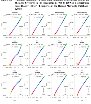
Figure 15: TL (solid black line) in fitted male mortality of the model of

(36)

(37)

(38)

For the standard Gompertz model _, (blue solid line) of Danish women in Figure 16, the relation of log temporal variance to log temporal mean is close to linear (as predicted by TL) except for the large values of the mean and variance of old-age mortality in the upper right corner of the graph. A fitted TL (dark blue solid line, log10

variance = –2.35 + 1.60 log10 mean) approximates the Gompertz log temporal variance

and log temporal mean closely over most of their range.

When _, changes linearly over time and _, is constant over time, _, gives a variance-mean relationship (red solid line) that approximates the Gompertz log variance and log mean closely but is slightly concave (on log–log coordinates). The average slope of this curve, estimated by

log / log ,

is 1.64, close to the slopeb = 1.60 of the fitted TL. Thus the second case considered above (Gompertz model with _, = and _, = ) gives an approximate explanation of the form and slope of the fitted TL.

By contrast, when _, is constant over time and _, changes linearly in time, the relationship of log variance of _, to log mean of _, , calculated numerically (green solid line) from _, , is visually indistinguishable from linear and has a numerically estimated slope indistinguishable from 2 (to a precision of at least five decimal places). These results confirm numerically the above mathematical analysis of Case 1. This case cannot explain the slope of the TL fitted either to observed mortality or to Gompertz model mortality.

In conclusion, in this example, the linear trend in and the linear trend in _, in combination explain qualitatively and quantitatively why TL for Gompertz-modeled mortality has slope notably less than 2, unlike the slope of exactly 2 that would be expected theoretically if _, were constant (regardless of whether _, is constant or changing in time).

4. Conclusion

4.1 Summary

(39)

(Figures 2 and A-1 in Bohk, Rau, and Cohen 2015; and Figures 3–4 here). This approximate linearity was consistent with Taylor’s law. Here we sought to explain this pattern.

We compared TL fitted to temporal means and temporal variances of observed mortality with TL fitted to mortality in the models of Gompertz (1825), Makeham (1860), and Siler (1979, 1983). These models have progressively more parameters and, in the same order, fit the age profile of observed mortality progressively more closely.

We analyzed how well each mortality model’s TL matched TL fitted to observed mortality by comparisons of three features: the log–log linearity of the temporal means and temporal variances of the modeled mortality, the age profile (defined as the set of pairs of log(temporal mean mortality at agex) and log(temporal variance of mortality at agex), for all agesx), and the slope.

For log–log linearity, we found that TL approximated mortality in the fitted models of Gompertz, Makeham, and Siler more closely than TL approximated observed mortality. As a consequence,r2_{values of TL of the Gompertz model were very close,}

and rounded, to 1. Compared to the Gompertz model, the models of Makeham and Siler resulted in closer fits to observed mortality and to the TL of observed mortality. Consequently, the r2_{values of TL of the models of Makeham and Siler were often}

slightly smaller than those of Gompertz but were also often closer to those of the observed mortality.

For the age profile of TL, we found that the TL of the Siler model fitted to observed mortality had an age profile that was closer to the age profile of TL of observed mortality than were the age profiles of TL of the fitted models of Makeham and Gompertz.

For the slopes of TL, we found that the TL of the Makeham model fitted to observed mortality had a slope that was closest to the slope of TL fitted directly to observed mortality, among the three models. Differences in the slope of TL between males and females in the fitted Makeham models were also closest to the differences in the slope of TL between males and females of observed mortality.

In addition to these empirical and statistical insights, we demonstrated mathematically that the log temporal means and log temporal variances of mortality in the Gompertz model satisfy TL exactly with slopeb = 2 and an explicitly determined intercept when the modal age at death in the Gompertz model increases linearly with time and theβt parameter for the increase of mortality with age is constant in timet (or

, is constant in time). As the Gompertz model is a special case of the more complex

models of Makeham and Siler, these theoretical findings also apply to certain parameter values of the other two models.

(40)

smaller than 2 (apart from the two exceptions noted above, for Gompertz model mortality of Russian males and Siler model mortality of French females). To explain why the slopes of TL fitted to observed mortality and the fitted models were notably smaller than 2 (with the two exceptions just noted), our computational experiments showed that, in the presence of a linearly increasing modal age at death, it was necessary and sufficient to take into account in the Gompertz model a linear trend in

, . When , increased linearly in time, the slope of TL based on Gompertz

mortality was less than 2, and when _, was constant, the slope of TL based on Gompertz mortality was numerically (and mathematically) indistinguishable from 2. We tested numerically and confirmed this explanation for women and men in 12 countries of the Human Mortality Database. These numerical results indicate that, as long as _, , the growth rate of mortality with age, increases linearly with time, TL fitted to mortality will have a slope that is not equal to 2.

To conclude, our empirical, statistical, mathematical, and numerical findings confirm that the temporal TL is a regular pattern rooted in widely recognized models of the age pattern and temporal evolution of human mortality.

4.2 Future research

These results raise further theoretical and empirical questions.

Our mathematical analysis of the Gompertz model remains incomplete when both parameters (the modal age at death and the growth rate of mortality with age) change in time. Our computational experiment gave clear results about this case, but we have not proved these results mathematically. Mathematical analysis is needed to reveal the necessary and sufficient conditions for TL fitted to Gompertz mortality to have a slope less than 2 (not merely different from 2).

It would be desirable to complete the mathematical analysis of the Gompertz model and to extend it to the Makeham, Siler, and other more complex models, for example, those of Heligman and Pollard (1980) and Thiele (1872), and piecewise constant mortality models of, for example, Brouhns, Denuit, and Vermunt (2002) and Cairns et al. (2009). These models may provide more precise approximations to empirical age profiles of mortality. However, their larger number of parameters and their greater mathematical complexity make them more difficult to analyze mathematically and to understand. Since our goal here was to understand an empirical pattern in a transparent way, we focused on simpler mortality models.

(41)

rates simultaneously, as in Brouhns et al. (2002), Cairns et al. (2009), and Renshaw and Haberman (2006), and reviewed by Booth and Tickle (2008). In a GLM approach, the dependent variable would be _, for all agesx, all yearst, both sexes, and all countries. The independent variables (predictors) would be age x, year t, sex (female or male), country, and various higher-order (e.g., x2_and_t2_{to model curvature) and interaction}

terms to be determined in the course of the analysis. The coefficients of predictort and

t2_{would quantify the importance of systematic trends, linear and nonlinear respectively.}

A GLM can estimate the mean and the variance of _, simultaneously (for example, by using quasi-likelihood techniques for the variance). With the estimates of means and variances of _, from a GLM, it would be possible to test TL with finer resolution than has been possible with the traditional approach used here, in which temporal means and temporal variances are computed independently for each age, sex, and country.

A GLM could also be used to analyze mortality from each of the three models considered here, and the structure and coefficients of the GLM for modeled mortality could be compared with the structure and coefficients of the GLM for observed mortality. This comparison would permit an evaluation of the models with finer resolution than has been possible with the traditional approach used here.

Testing TL in deterministic mortality models is a special case of applying TL to smoothed data, with some of the initial variability removed, leaving only dominant trends. Here the ‘smoothed data’ are the predictions of the models. Comparison of the goodness of fit and parameter estimates of TL with such smoothed data versus with the original data shows whether the smoothed trends or the variability about those trends dominate the goodness of fit and parameter estimates of TL. In the examples in this paper, because the TL fitted to models is generally close to the TL fitted to the original mortality observations, it is clear that the smoothed trends play the dominant role in the success of TL. Further research is needed to show the conditions under which the smoothed data versus the fluctuations around trends dominate the performance of TL.

(42)

generalizing the Gompertz and other models to allow for stochastic fluctuations in mortality over time.

Reviewer Hal Caswell posed a more general theoretical question that is also related to variation in mortality. Temporal fluctuations in mortality rates are a component of a demographic model in a stochastic environment. What are the consequences for stochastic population growth of greater temporal variance in mortality at (older) ages where the mean mortality is also higher? This question shows the potential use of TL applied to mortality in modeling and simulating stochastic age-structured populations.

The above outlines of potential applications of TL in human mortality indicate TL’s possible usefulness and relevance in formal and empirical demographic research.

5. Acknowledgments

(43)

References

Bergeron-Boucher, M.P., Ebeling, M., and Canudas-Romo, V. (2015). Decomposing changes in life expectancy: Compression versus shifting mortality.Demographic Research 33(14): 391–424.doi:10.4054/DemRes.2015.33.14.

Bohk, C., Rau, R., and Cohen, J.E. (2015). Taylor’s power law in human mortality.

Demographic Research 33(21): 589–610.doi:10.4054/DemRes.2015.33.21. Bongaarts, J. (2005). Long-range trends in adult mortality: Models and projection

methods.Demography 42(1): 23–49.doi:10.1353/dem.2005.0003.

Booth, H. and Tickle, L. (2008). Mortality modelling and forecasting: A review of methods. Annals of Actuarial Science 3(1–2): 3–43. doi:10.1017/S17484995 00000440.

Brouhns, N., Denuit, M., and Vermunt, J.K. (2002). A Poisson log-bilinear regression approach to the construction of projected lifetables.Insurance: Mathematics and Economics 31(3): 373–393.doi:10.1016/S0167-6687(02)00185-3.

Cairns, A.J.G., Blake, D., Dowd, K., Coughlan, G.D., Epstein, D., Ong, A., and Balevich, I. (2009). A quantitative comparison of stochastic mortality models using data from England and Wales and the United States. North American Actuarial Journal 13(1): 1–35.doi:10.1080/10920277.2009.10597538.

Canudas-Romo, V. (2008). The modal age at death and the shifting mortality hypothesis. Demographic Research 19(30): 1179–1204. doi:10.4054/DemRes. 2008.19.30.

Canudas-Romo, V. (2010). Three measures of longevity: Time trends and record values.Demography 47(2): 299–312.doi:10.1353/dem.0.0098.

Christensen, K., Doblhammer, G., Rau, R., and Vaupel, J.W. (2009). Ageing populations: The challenges ahead. The Lancet 374(9696): 1196–1208.

doi:10.1016/S0140-6736(09)61460-4.

Cohen, J.E. (2013). Taylor’s power law of fluctuation scaling and the growth-rate theorem.Theoretical Population Biology 88: 94–100.doi:10.1016/j.tpb.2013.04. 002.

(44)

Cohen, J.E., Xu, M., and Brunborg, H. (2013). Taylor’s law applies to spatial variation in a human population.Genus69(1): 25–60.

Eisler, Z., Bartos, I., and Kertész, J. (2008). Fluctuation scaling in complex systems: Taylor’s law and beyond. Advances in Physics 57(1): 89–142. doi:10.1080/ 00018730801893043.

Gompertz, B. (1825). On the nature of the function of the law of human mortality, and on a new mode of determining the value of life contingencies. Philosophical Transactions of the Royal Society of London 115: 513–583. doi:10.1098/rstl. 1825.0026.

Grigoriev, P., Doblhammer-Reiter, G., and Shkolnikov, V. (2013). Trends, patterns, and determinants of regional mortality in Belarus, 1990–2007. Population Studies

67(1): 61–81.doi:10.1080/00324728.2012.724696.

Grigoriev, P., Vladimir S., Andreev, E.M., Jasilionis, D., Jdanov, D., Meslé, F., and Vallin, J. (2010). Mortality in Belarus, Lithuania, and Russia: Divergence in recent trends and possible explanations. European Journal of Population 26: 245–274.doi:10.1007/s10680-010-9210-1.

Heligman, L. and Pollard, J.H. (1980). The age pattern of mortality. Journal of the Institute of Actuaries107: 49–80.doi:10.1017/S0020268100040257.

Horiuchi, S., Ouellette, N., Cheung, S.L.K., and Robine, J.M. (2013). Modal age at death: Lifespan indicator in the era of longevity extension. Vienna Yearbook of Population Research11: 37–69.doi:10.1553/populationyearbook2013s37. Human Mortality Database (2015). Berkeley and Rostock: University of California and

Max Planck Institute for Demographic Research.www.mortality.org.

Kendal, W.S. (2004). Taylor’s ecological power law as a consequence of scale invariant exponential dispersion models.Ecological Complexity1: 193–209.doi:10.1016/ j.ecocom.2004.05.001.

Kendal, W.S. (2013). Fluctuation scaling and 1/f noise: Shared origins from the Tweedie family of statistical distributions.Journal of Basic and Applied Physics

2(2): 40–49.doi:10.5963/JBAP0202002 .

Kendal, W.S. and Jørgensen, B. (2011). Taylor’s power law and fluctuation scaling explained by a central-limit-like convergence.Physical Review E 83(6): 066115.

doi:10.1103/PhysRevE.83.066115.

(45)

Kilpatrick, A.M. and Ives, A.R. (2003). Species interactions can explain Taylor’s power law for ecological time series.Nature422: 65–68.doi:10.1038/nature01471. Makeham, W.M. (1860). On the law of mortality and the construction of annuity tables.

The Assurance Magazine, and Journal of the Institute of Actuaries 8(6): 301– 310.doi:10.1017/S204616580000126X.

Missov, T.I., Lenart, A., Nemeth, L., Canudas-Romo, V., and Vaupel, J.W. (2015). The Gompertz force of mortality in terms of the modal age at death. Demographic Research 32(36): 1031–1048.doi:10.4054/DemRes.2015.32.36.

Mullen, K., Ardia, D., Gil, D., Windover, D., and Cline, J. (2011). DEoptim: An R package for global optimization by differential evolution. Journal of Statistical Software 40(6): 1–26.doi:10.18637/jss.v040.i06.

Oksuzyan, A., Juel, K., Vaupel, J.W., and Christensen, K. (2008). Men: Good health and high mortality: Sex differences in health and aging. Aging Clinical and Experimental Research20(2): 91–102.doi:10.1007/BF03324754.

Rau, R., Jasilionis, D., Soroko, E.L., and Vaupel, J.W. (2008). Continued reductions in mortality at advanced ages. Population and Development Review 34(4): 747– 768.doi:10.1111/j.1728-4457.2008.00249.x.

R Core Team (2015). R: A language and environment for statistical computing. Vienna: R Foundation for Statistical Computing.http://www.R-project.org/.

Renshaw, A.E. and Haberman, S. (2006). A cohort-based extension to the Lee–Carter model for mortality reduction factors. Insurance: Mathematics and Economics

38(3): 556–570.doi:10.1016/j.insmatheco.2005.12.001.

Shkolnikov, V.M., Andreev, E.M., McKee, M., and Leon, D.A. (2013). Components and possible determinants of the decrease in Russian mortality in 2004–2010.

Demographic Research 28(32): 917–950.doi:10.4054/DemRes.2013.28.32. Siler, W. (1979). A competing-risk model for animal mortality. Ecology 60(4): 750–

757.doi:10.2307/1936612.

Siler, W. (1983). Parameters of mortality in human populations with widely varying life spans.Statistics in Medicine2: 373–380.doi:10.1002/sim.4780020309.

Taylor, L.R. (1961). Aggregation, variance and the mean. Nature 189: 732–735.

(46)

Thiele, T.N. (1872). On a mathematical formula to express the rate of mortality throughout the whole of life, tested by a series of observations made use of by the Danish Life Insurance Company of 1871. Journal of the Institute of

Actuaries and Assurance Magazine 16(5): 313–329. doi:10.1017/S20461674

00043688.

Tippett, M.K. and Cohen, J.E. (2016). Tornado outbreak variability follows Taylor’s power law of fluctuation scaling and increases dramatically with severity.

Nature Communications 7: 10668.doi:10.1038/ncomms10668.

Vaupel, J.W. (2010). Biodemography of human ageing. Nature 464: 536–542.

doi:10.1038/nature08984.

Xiao, X., Locey, K.J., and White, E.P. (2015). A process-independent explanation for the general form of Taylor’s law. American Naturalist 186(2): E51–E60.

(47)

Appendix 1: Taylor’s law with slope 2 describes the Gompertz model

Theorem

The Gompertz mortality model with modal age at death increasing linearly in time obeys a cross-age-scenario of Taylor’s law (TL) exactly with slopeb = 2. Explicitly, assuming the Gompertz model _, at agex and timet,

, = ( ), > 0, > 0, for = 1, … , , = 1, … , ,

with a linear change (increase or decrease) over time in the modal age at death,

= + ⋅ > 0, > 0, ≠ 0, for = 1, … , ,

and an exponential rate increase of mortality with agex that is constant over timet,

= > 0, for = 1, … , ,

then TL holds with slope 2 and intercept log( − ) − 2 log on log–log coordinates:

log ( ) = log + 2 ⋅ log ( ),for = 1, … , ,

where the positive constants , are defined below.

Proof

From the assumptions,

, = ( )= ( { ⋅ })= ( ) ,

which implies that _, is an exponentially increasing function of agex for every timet. It also implies that _, is an exponentially decreasing function of timet for every agex

(48)

( ) =1 , =1 ( ) = ,

where the first factor varies with agex only and the bracketed second factor varies with timet andT only. Define

≡ , ≡ .

does not depend on agex. Then since > 0, ≠ 0, we have < 1 ifw > 0 andq > 1 ifw < 0 and in both cases

= ( + + ⋯ + ) = (1 + + ⋯ + )

= ⋅ (1 −_{1 −} ).

Since > 0, ( ) = increases exponentially at rateβ with increasingx. Also

( ) =1 , − ( ) =1 , − ( )

=1 ( ) ₋

= − .

Define

≡ .

(49)

= ( ⋅ ₊ ⋅ _{+ ⋯ +} ⋅ _{) =} (1 − ⋅( ))

1 − .

Also

( ) = ( − ) .

By Cauchy’s inequality, − > 0. Therefore ( ) increases exponentially at rate 2β with increasing agex. Thus, we showed that

( ) = ,

( ) = ( − ) .

Therefore

( ) = ( ) .

Appendix 2: Taylor’s law with slope less than 2 describes the model

of Makeham

In the Makeham model, eq. (2), the additivity of expectations yields

( ) = ( ) + ( ) _{= ( ) + ( )}_.

The subscript M denotes the Makeham model, and the subscript G denotes the Gompertz model. Calculating the variance in the Makeham model requires specifying the relation between and ( ). Based on the parameter estimates of the Makeham model in Figures A-5–A-10, we examine this empirically plausible special case:

= , > 0, > 0, = > 0,

= + ⋅ > 0, > 0, > 0.

Thus

(50)

On the right side, the first term depends only ont, not onx, and the second term factors into one factor that depends onx only and another factor that depends ont

only. By summing geometric series as in Appendix 1, we can get explicit expressions for the constant (and is identical to that constant in the Gompertz model) in the expression

( ) = + .

With increasing agex, ( ) grows as the factor . Also,

, = + { ⋅ }+ 2 { ⋅ } .

Therefore

, = + + ,

( ) = + + 2 ,

( ) = , − ( )

= − + ( − ) + ( − 2 ) .

The same elementary methods used in Appendix 1 can determine and explicitly.

From Figures A-7–A-8, ≈ 0.1 for both females and males. Hence asx increases from 0 to 100, increases from = 1 to approximately ≈ 2.2 × 10 . Hence the term of ( ) that contains the factor , which is approximately ≈ 4.8 × 10 when x = 100, increasingly dominates the term of ( ) that contains the factor . So, to a first approximation, neglecting all but the dominant terms,

( ) scales with increasing agex as the square of ( ). Thus, asymptotically for increasing agex, TL holds approximately with slope ≈ 2.

(51)

(52)

(53)

(54)

(55)

(56)

(57)

(58)

(59)

(60)

(61)