___________________
E-mail address: [email protected] Received April 22, 2016
Available online at http://scik.org
J. Math. Comput. Sci. 8 (2018), No. 1, 98-113 https://doi.org/10.28919/jmcs/2757
ISSN: 1927-5307
DEVELOPMENT OF A DISCRETE SIMULATION MODEL FOR TSUNAMI TIDAL WAVE
OBAYOMI ABRAHAM ADESOJI
Department of Mathematical Sciences, Faculty of Science, Ekiti State University, P. M. B 5363, Ado-Ekiti, Nigeria
Copyright © 2018 Obayomi Abraham Adesoji. This is an open access article distributed under the Creative Commons Attribution License, which permits unrestricted use, distribution, and reproduction in any medium, provided the original work is properly cited.
Abstract. In this paper, we develop new discrete models for the numerical simulation of non-linear ordinary differential equation arising from the dynamics of a tidal wave. A new set of non-standard schemes are proposed using the technique of non-local approximation. Both one step and two step formats have been considered. The schemes were found to be suitable for the numerical simulation of the Tsunami equation as proposed.
Keywords: discrete simulation model; Tsunami tidal wave. 2010 AMS Subject Classification: 81T80.
Introduction
One of the most important questions in prognostic tsunami modeling is estimation of tsunami
run-up heights at different points along the coastline. Methods for numerical simulation of
tsunami wave propagation are well developed and are widely used by a great number of
scientists. To date, only a few existing numerical models have met current standards, and these
models remain the only choice for use for real-world forecasts
To some earlier modelers, the Tsunamis are assumed to be linear, long gravity waves at single
frequencies. Several models that have proven very useful has employed non-linear views. Some
of these works include: [1],[2],[3],[4],[5] and[6]. Since numerical applications has proven to
apply numerical experiments to simulate various scenario possible for any given dynamical
system
A lot of work has been done in the area of numerical modeling of ordinary differential
equations. Many of these techniques have been found to be useful for developing discrete
solution for different type of equations.
Various researchers have come up with useful models in which the numerical simulations have
been applied in the management and study of tidal waves among them are: [7],[8],[9],[10]
and[11].
In this work we will use a combination of non-local approximation of the derivatives and the
grid point estimates to develop one step and two step Non-standard finite difference schemes
for the Tsunami equation.
Non-local approximations and renormalization of the denominator functions have been found to
be appropriate for the solution of differential equations. The works of [12] and [13], [14],[15]
and [16] have used these techniques extensively to develop discrete models that correctly follow
the dynamics of the original differential equation. In many cases the schemes have been found
to possess certain desirable qualitative properties like monotonicity of solutions. linear stability
and preservation of the properties of the fixed points. The model of non-linear ordinary
differential equation proposed in the book of [17] will be used for the numerical experiment. The
significant of this numerical model is in the combination of several techniques in one scheme to
simulate the original equation. Some denominator functions developed by these authors have
been used for the purpose of comparison. These denominator functions have been developed
based on the rule 2 of non-standard modeling technique proposed by [12].
2. The Tsunami model (Gill and Cullen 2005)
The Tsunami Model is given by
dy
dx= y√4 − 2y (1)
y(x) > 0 is the height of the wave expressed as a function of its position relative to a point
off-sore. This is one of the simplest model for a tidal wave considering the complex dynamics of the
phenomena being model. The function y(x) has a lot of underlining assumption and as such in
reality may possess more complex properties. The equilibrium points of this equation are y= 0
if y0 = 2 the analytic solution is y(x) = 2sech2x Otherwise y(x) = 2sech2(x − c) (2)
We will develop new schemes that possess the same qualitative properties as that of this
differential equation.
3. Derivation of the Method
We will apply rule2&3 (see [12]) and their extensions in [14] to each of the components of the
equation as shown below
Rule 2 (Mickens 1994)
Denominator function for the discrete derivatives must be expressed in terms of more
complicated function of the step-sizes than those conventionally used. This rule allows the
introduction of complex analytic function of h that satisfy certain conditions in the denominator . It must be stated here that the selection of an appropriate denominator is an ‘art’ (Mickens 1999).
Close examinations of differential equation, for which the exact schemes are known, shows that
the denominator function generally are functions that are related to particular solutions or
properties of general solution to the differential equation. This therefore places great importance
on the necessity of the modeler to obtain as much analytic knowledge as possible about the
differential equation. A lot of such denominator functions have been developed by this author
and many others, such will be used directly here.
Rule 3 (Mickens 1994)
The non-linear terms must in general be modeled (approximated) non-locally on the
computational grid or lattice in many different ways.
Application of the combination of these two rules will give us the following transformations
dy dx ≡
(𝑦𝑘+1−yk)
𝜓 where 𝜓(ℎ) → ℎ + 0(ℎ
2)𝑎𝑠ℎ → 0 (3)
dy dx ≡
(𝑦𝑘+1−𝛽yk)
𝜓 where 𝜓(ℎ) → ℎ + 0(ℎ
2), 𝛽(ℎ) → 1 𝑎𝑠ℎ → 0 (4)
dy dx ≡
(𝑦𝑘+1−𝛽yk−1)
2𝜓 where 𝜓(ℎ) → ℎ + 0(ℎ
2), 𝛽(ℎ) → 1 𝑎𝑠ℎ → 0 (5)
The following non-local approximations
𝑦𝑘+1 ≡
(𝑦𝑘+1+𝛽yk)
2 where 𝛽(ℎ) → 1 𝑎𝑠ℎ → 0 (6)
𝑦𝑘+1 ≡
(2𝑦𝑘+𝛽yk−1)
3 where 𝛽(ℎ) → 1 𝑎𝑠ℎ → 0 (7)
𝑦𝑘+1 ≡ (𝑦𝑘 yk)
𝑦𝑘+1 ≡ 𝑎𝑦𝑘+1+ 𝑏𝑦𝑘 𝑎 + 𝑏 = 1 (9)
Sample renormalisation functions to be employed are
𝜓 =sin (∝ ℎ) , ∝ϵ R → ℎ + 0(ℎ2) 𝑎𝑠 ℎ → 0 (10)
𝜓 = (𝑒 𝜆h−1)
𝜆 , λϵ R , → ℎ + 0(ℎ
2) 𝑎𝑠 ℎ → 0 (11)
𝛽 = 𝑐𝑜𝑠(∝ ℎ), ∝ϵ R → 1 𝑎𝑠 ℎ → 0 (12)
4. Derivation of the schemes
dy
dx= y√4 − 2y (Zill &Cullen 2005) (13)
One step Schemes
Scheme A
Applying non-local approximation to grid points using the transformation equations (3)and(9) in
(1)
we have the following
𝑦𝑘+1−𝑦𝑘
𝜓 = (𝑎𝑦𝑘+1+ 𝑏𝑦𝑘)√(4 − 2𝑦𝑘) (14)
𝑦𝑘+1= 𝑦𝑘 + (𝑎𝜓𝑦𝑘+1+ 𝑏𝜓𝑦𝑘)√(4 − 2𝑦𝑘) (15)
𝑦𝑘+1=
𝑦𝑘(1+𝑏𝜓)√(4−2𝑦𝑘)
(1−𝑎𝜓)√(4−2𝑦𝑘) (16)
We can choose any 𝜓 to form schemes of the form
𝑦𝑘+1=
𝑦𝑘(1+𝑏𝜓)√(4−2𝑦𝑘)
(1−𝑎𝜓)√(4−2𝑦𝑘) , 𝜓 = ℎ ,𝛽 = 𝑐𝑜𝑠(∝ ℎ), λ,
∝ϵ R Scheme A1 (17)
𝑦𝑘+1= 𝑦𝑘(1+𝑏𝜓)√(4−2𝑦𝑘)
(1−𝑎𝜓)√(4−2𝑦𝑘) , 𝜓 =
(𝑒𝜆h−1)
𝜆 𝛽 = 𝑐𝑜𝑠(∝ ℎ), λ,∝ϵ R Scheme A2
(18)
𝑦𝑘+1=
𝑦𝑘(1+𝑏𝜓)√(4−2𝑦𝑘)
(1−𝑎𝜓)√(4−2𝑦𝑘) , 𝜓 = sin (h) ,𝛽 = 𝑐𝑜𝑠(∝ ℎ), λ,
∝ϵ R Scheme A3 (19)
Scheme B
Applying non-local approximation to derivative using the transformation equations (3) in (1)
𝑦𝑘+1−𝛽𝑦𝑘
𝜓 = √𝑦𝑘
2(4 − 2𝑦
𝑘) (20)
𝑦𝑘+1= 𝛽𝑦𝑘+ 𝜓𝑦𝑘√(4 − 2𝑦𝑘) (21)
We can choose any 𝜓 to form schemes of the form
𝑦𝑘+1= 𝛽𝑦𝑘+ 𝜓𝑦𝑘√(4 − 2𝑦𝑘), 𝜓 = ℎ ,𝛽 = 𝑐𝑜𝑠(∝ ℎ), λ,∝ϵ R Scheme B1 (22)
𝑦𝑘+1= 𝛽𝑦𝑘+ 𝜓𝑦𝑘√(4 − 2𝑦𝑘), 𝜓 =
(𝑒𝜆h−1)
𝜆 𝛽 = 𝑐𝑜𝑠(∝ ℎ), λ,∝ϵ R Scheme B2 (23) 𝑦𝑘+1= 𝛽𝑦𝑘+ 𝜓𝑦𝑘√(4 − 2𝑦𝑘), 𝜓 = sin (h) ,𝛽 = 𝑐𝑜𝑠(∝ ℎ), λ,∝ϵ R Scheme B3 (24)
The direct substitution of a normalized denominator to replace h in the standard
Finite Difference Scheme𝑦𝑘+1= 𝑦𝑘+ ℎ𝑓( 𝑥𝑘, 𝑦𝑘), will result in the simple scheme given below in
(25).
This scheme will not involve the application of any other Nonstandard modeling rule except the
replacement of the denominator.
𝑦𝑘+1= 𝑦𝑘+ 𝜓𝑦𝑘√(4 − 2𝑦𝑘), 𝜓 =
(𝑒𝜆h−1)
𝜆 Scheme (DIRECT) (25)
Two Step Schemes
Method I
Scheme C
Applying non-local approximation to the original differential equation using the transformation
equations (5) in (1) we obtain the following
𝑦𝑘+1−𝛽𝑦𝑘−1
2𝜓 = √𝑦𝑘
2(4 − 2𝑦
𝑘) (26)
𝑦𝑘+1= 𝛽𝑦𝑘−1+ (2𝜓𝑦𝑘)√(4 − 2𝑦𝑘) (27)
We can choose any 𝜓 to form schemes of the form
𝑦𝑘+1= 𝛽𝑦𝑘−1+ (2𝜓𝑦𝑘)√(4 − 2𝑦𝑘) , 𝜓 = ℎ ,𝛽 = 𝑐𝑜𝑠(∝ ℎ), λ,∝ϵ R Scheme C1 (28)
𝑦𝑘+1= 𝛽𝑦𝑘−1+ (2𝜓𝑦𝑘)√(4 − 2𝑦𝑘), 𝜓 = (𝑒𝜆h−1)
𝜆 𝛽 = 𝑐𝑜𝑠(∝ ℎ), λ,∝ϵ R Scheme C2 (29) 𝑦𝑘+1= 𝛽𝑦𝑘−1+ (2𝜓𝑦𝑘)√(4 − 2𝑦𝑘), 𝜓 = sin (h) ,𝛽 = 𝑐𝑜𝑠(∝ ℎ), λ,∝ϵ R Scheme C3 (30)
Note that 𝜓 = ℎ is the standard denominator function in Finite difference method
We will also compute values for the scheme
Definition 1: An initial value problem of a first order ODE can be represented as follows:
y′= f(t, y) , у(t
where y0 is the value of y at time t0
It is common fact to write the functional dependence 𝑦𝑛+1on the quantities 𝑥𝑛,𝑦𝑛 and h in the form;
yn+1 = yn + h φ( 𝑥𝑛, 𝑦𝑛; ℎ) (32)
Where φ( 𝑥𝑛, 𝑦𝑛; ℎ) is called the increment function.
Let us denote 𝑦𝑘 the approximate solution of (31) at grid point 𝑡𝑘 : 𝑦𝑘 = 𝑦(𝑡𝑘) then the sequence 𝑦𝑘 is obtained as a solution to a finite difference equation of the form (32). Lets denote
(32) by the sequence 𝑦𝑘= 𝐹(ℎ ; 𝑦𝑘) (33 )
Definition 2: (Anguelov and Lubuma(2003).) Assume that the solution of equation (31) satisfy some
property 𝓟,The numerical scheme(32) is called qualitatively stable with respect to property 𝓟 or 𝓟-stable, if for every value h˃0 the set of solutions of (32) satisfies 𝓟.
Definition 3: (Anguelov and Lubuma(2003)) A set G(ῼ) of real-valued functions defined on a subset ῼ
of [t0,∞) monotonically depend on the initial value(at t0) if for every two functions y,zЄ G(ῼ) we have
y(t0) ≤ z(t0) ⇒ y(t) ≤ z(t), t Є ῼ (34)
Definition 4: (Anguelov and Lubuma(2003): The finite difference scheme(33) is stable with respect to
the property of monotonicity of solutions if for every y0 Єℝ the solution yk of (33) is an increasing or a
decreasing sequence according as the y(t) of equation (31) is increasing or decreasing.
Definition 5: (Anguelov and Lubuma(2003): The finite difference method (32) is called elementary
stable if for any value of the step size h , its only fixed points ӯ are those of the differential equation (31), the linear stability property of each ӯ being the same for both the differential equation and the discrete
method.
The following theorems establish the conditions (sufficient) for the stability properties of the
discrete equation (33). Proves of the theorems can be found in (Anguelov and Lubuma(2003)) .
The authors have been able to prove the condition for stability of the fixed points and link the
properties of linear stability to elementary stability of the fixed points.
Theorem 1: (Anguelov and Lubuma(2003): The difference Scheme (32) is stable with respect to
monotone dependence on initial value if
𝜕𝐹
𝜕𝑦(ℎ; 𝑦) ≥ 0, 𝑦Єℝ, ℎ˃0 (35)
Theorem 2: (Anguelov and Lubuma(2003): Assume that the difference scheme (32) is stable with
y = F(h ; y) and f(y)= 0 (36)
in y have the same roots considered their multiplicity. Then the difference scheme (33) is stable with
respect to monotonicity of solutions.
Theorem 3: (Anguelov and Lubuma(2003)): Under the assumptions of theorem (2) the difference
scheme (32) is elementary stable.
In the next subsection section we shall use the above theorems (1 –3) to establish the stability or
otherwise of the non-exact schemes developed for the Logistic and Combustion equations. Please note
that a major advantage of having an exact scheme for a differential equation is that questions related to
the usual considerations of consistency, stability and convergence do not arise (see Mickens 1994).
In this Section we show that our schemes satisfy the sufficient condition for the stability properties
described above.
Stability of Scheme A with respect to monotonicity of solutions.
𝑦𝑘+1=
𝑦𝑘(1+𝑏𝜓)√(4−2𝑦𝑘)
(1−𝑎𝜓)√(4−2𝑦𝑘) (37)
𝑦 = 𝐹(ℎ, 𝑦) = 𝑦𝑘(1+𝑏𝜓)√(4−2𝑦𝑘)
(1−𝑎𝜓)√(4−2𝑦𝑘) (38)
𝑦 = 𝐹(ℎ, 𝑦) = 𝑦(1+𝑏𝜓)√(4−2𝑦)
(1−𝑎𝜓)√(4−2𝑦) (39)
𝑦(1 − 𝑎𝜓)√(4 − 2𝑦) − 𝑦(1 + 𝑏𝜓)√(4 − 2𝑦) = 0 (40)
Have roots 0 and 2
Let 𝑦 ≠ 0 𝑎𝑛𝑑 𝑦 ≠ 2
𝑙𝑒𝑡 𝑎 + 𝑏 = 1
(1 − 𝑎𝜓)√(4 − 2𝑦) = (1 + 𝑏𝜓)√(4 − 2𝑦) (41)
𝑏𝜓 = −𝑎𝜓
𝑏 = −𝑎 (42)
This contradicts the assumption of selecting parameters 𝑎, 𝑏 𝑠. 𝑡. 𝑎 + 𝑏 = 1
Hence the only roots of 𝑦 = 𝐹(ℎ, 𝑦) is 0 and 2
𝑓(𝑦) = 𝑦√(4 − 2𝑦) have roots 0 and 2
The conditions of theorem…. are satisfied for all scheme A
Stability of Scheme B&C with respect to monotonicity of solutions.
𝑦𝑘+1= 𝛽𝑦𝑘+ 𝜓𝑦𝑘√(4 − 2𝑦𝑘) (43)
𝑦 = 𝐹(ℎ, 𝑦) = 𝛽𝑦 + 𝜓𝑦√(4 − 2𝑦) (44)
𝑦 − 𝛽𝑦 − 𝜓𝑦√(4 − 2𝑦) = 0 have root 0
It will have root 2 iff 𝛽 = 1
Hence if 𝛽 = cos (ℎ) and ℎ ≠ 0
and 𝑓(𝑦) = 𝑦√(4 − 2𝑦) have roots 0 and 2
The condition of theorem 2 is not satisfied we cannot conclude on the property of monotonicity of
solutions.
However the Scheme given by
𝑦𝑘+1= 𝑦𝑘 + 𝜓𝑦𝑘√(4 − 2𝑦𝑘) (45)
Clearly satisfy the conditions of theorem 2 and we conclude that the scheme Direct has the property of
monotonicity of solutions
The above also confirm Elementary Stability as stated in Theorem 3.
Stability of Scheme A with respect to monotone dependence on initial values of solutions.
𝜕𝐹
𝜕𝑦(ℎ; 𝑦) ≥ 0
𝐹(ℎ, 𝑦) = 𝑦(1+𝑏𝜓)√(4−2𝑦)
(1−𝑎𝜓)√(4−2𝑦) (46)
Let ∝= (1 + 𝑏𝜓)and 𝛽 = (1 − 𝑎𝜓)
⇒ 𝐹(ℎ, 𝑦) = 𝑦∝√(4−2𝑦) 𝛽√(4−2𝑦) 𝜕𝐹
𝜕𝑦(ℎ; 𝑦) = −∝ 𝛽𝑦 − 𝛽[−∝ 𝑦+∝ (4 − 2𝑦)] (47)
= −∝ 𝛽 + 𝛽 ∝ 𝑦−∝ 𝛽(4 − 2𝑦)
⇒ −∝ 𝛽(4 − 2𝑦)≥0 (48)
⇒−∝ 𝛽≥0
⇒ −(1 + 𝑏𝜓)(1 − 𝑎𝜓)≥0 (49)
⇒1 + (1 − 𝑎)𝜓 ≤ 0 𝑎 + 𝑏 = 1
⇒(1 − 𝑎)𝜓 ≤ −1
⇒1 − 𝑎 ≤ −1 𝜓 ⇒𝑎 ≥1 +1
𝜓 and 𝑏 ≤ − 1
𝜓 (51)
Suppose (1 + 𝑏𝜓)≥ 0 AND (1 − 𝑎𝜓) ≤0
⇒𝑎 ≥1
𝜓 and 𝑏 ≤ 1 − 1
𝜓 (52)
The condition for theorem is satisfied with equation (50) and the second condition is contained in the first
for 𝜓 >0
Stability of Scheme B&C with respect to monotone dependence on initial values of solutions.
𝐹(ℎ, 𝑦) = 𝛽𝑦 + 𝜓𝑦√(4 − 2𝑦) (53)
𝜕𝐹
𝜕𝑦(ℎ; 𝑦) ≥ 0 𝜕𝐹
𝜕𝑦(ℎ; 𝑦) = 𝛽 − 𝜓𝑦
√(4−2𝑦)≥ 0 (54)
Let 𝑦 ≠ 0 𝑎𝑛𝑑 𝑦 ≠ 2 and 𝑦 > 0
⇒ 𝛽 ≥ 𝜓𝑦 √(4−2𝑦)
⇒ 𝛽√(4 − 2𝑦) ≥ 𝜓𝑦 (55)
Taking the positive root , the above is true for 0< 𝑦 < 2, 𝛽 = cos (ℎ), 𝜓 as defined
𝜕𝐹
𝜕𝑦(ℎ; 𝑦) ≥ 0 , for 0< 𝑦 < 2
This is also true when 𝛽 = 1
⇒ The Direct Scheme 𝑦𝑘+1= 𝑦𝑘 + 𝜓𝑦𝑘√(4 − 2𝑦𝑘) (56)
Satisfies
𝜕𝐹
𝜕𝑦(ℎ; 𝑦) ≥ 0 , for 0< 𝑦 < 2
NUMERICAL EXPERIMENT
The schemes have been tested using step size h=0.01 and for about 100 iterations. The result of
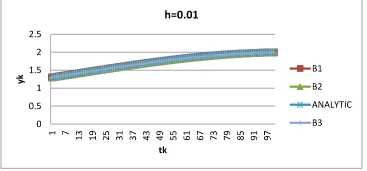
Fig 1: Graph of scheme A with the Analytic solution
Fig 2: Graph of Error of deviation of scheme A from the Analytic solution
Fig 3: Graph of scheme B with the Analytic solution 0
0.5 1 1.5 2 2.5
1 7 13 19 25 31 37 43 49 55 61 67 73 79 85 91 97
yk
tk
h=0.01
A1
A2
ANALYTIC
A3
0 0.01 0.02 0.03 0.04
1 6 11 16 21 26 31 36 41 46 51 56 61 66 71 76 81 86 91 96
Er
ro
r
tk
h=0.01
ERR A1
ERR A2
ERR A3
0 0.5 1 1.5 2 2.5
1 7 13 19 25 31 37 43 49 55 61 67 73 79 85 91 97
yk
tk
h=0.01
B1
B2
ANALYTIC
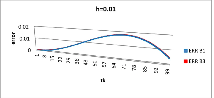
Fig 4: Graph of Error of deviation of scheme B from the Analytic solution
Fig 5: Graph of Error of deviation of scheme B1andB2 from the Analytic solution
Fig 6: Graph of Error of deviation of scheme B1 and B2 from the Analytic solution 0
0.005 0.01 0.015 0.02 0.025
1 7 13 19 25 31 37 43 49 55 61 67 73 79 85 91 97
Er
ro
r
o
f d
e
vi
ation
t
h=0.01
ERRB1
ERRB2
ERRB3
0 0.005 0.01 0.015 0.02 0.025
1 7 13 19 25 31 37 43 49 55 61 67 73 79 85 91 97
Er
ro
r
o
f d
e
vi
ation
t
h=0.01
ERRB1
ERRB2
0 0.01 0.02
1 8
15 22 29 36 43
50 57 64
71 78 85
92 99
e
rr
o
r
tk
h=0.01
ERR B1
Fig 7: Graph of Error of deviation of scheme A and B from the Analytic solution
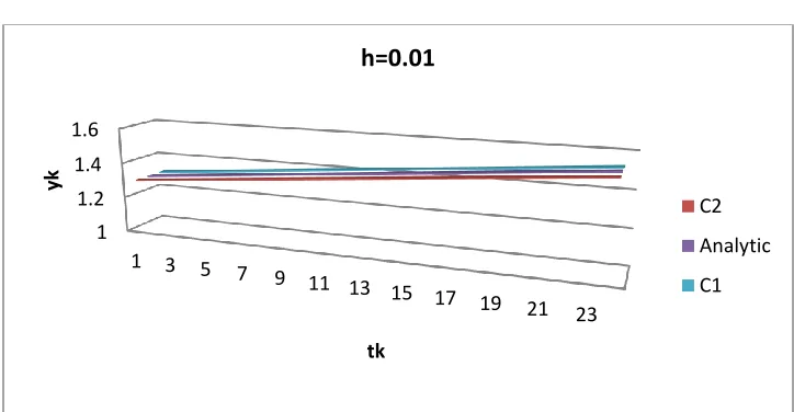
Fig 8: Graph of scheme C AND the Analytic solution
Fig 9: Graph of scheme C AND the Analytic solution (25 Iterations) 0
0.005 0.01 0.015 0.02 0.025 0.03 0.035
1 7 13 19 25 31 37 43 49 55 61 67 73 79 85 91 97
A
b
solut
e
E
rr
o
r
tk
h=0.01
ERRA1
ERRA2
ERRA3
ERRB1
ERRB2
ERRB3
0 0.5 1 1.5 2 2.5
1 7 13 19 25 31 37 43 49 55 61 67 73 79 85 91 97
yk
tk
h=0.01
C2
Analytic
C1
1 1.2 1.4 1.6
1 3 5
7 9
11 13 15 17 19 21 23
yk
tk
h=0.01
C2
Analytic
Fig 10: Graph of Error of deviation of scheme C from the Analytic solution
Fig 11: Graph of scheme A,B,C , Scheme Direct AND the Analytic solution
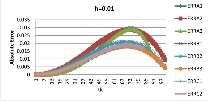
Fig 12: Graph of Error of deviation of scheme A, B and C from the Analytic solution 0 0.005 0.01 0.015 0.02 0.025
1 7 13 19 25 31 37 43 49 55 61 67 73 79 85 91 97
Er ro r tk h=0.01 ERR C2 ERR C1 0 0.5 1 1.5 2 2.5
1 7 13 19 25 31 37 43 49 55 61 67 73 79 85 91 97
yk tk h=0.01 DIRECTe x A1 A2 A3 B1 B2 B3 0 0.005 0.01 0.015 0.02 0.025 0.03 0.035
1 7 13 19 25 31 37 43 49 55 61 67 73 79 85 91 97
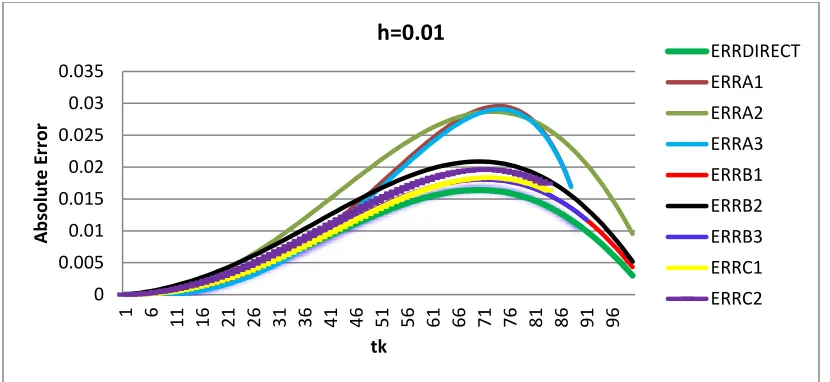
Fig 13: Graph of Error of deviation of scheme Direct, A, B & C from the Analytic solution
DISCUSSION AND CONCLUSION
We observe that the one step Finite Difference schemes (A and B) performed better as a
nonstandard scheme because the curves followed correctly the monotonicity of the solution
of the original equation (see fig 2,3,4 and 13). The schemes of B and Scheme (DIRECT),
also produce the smallest absolute error of deviation (see fig 5,7,13). We also observed that
the two step scheme (C) also perform well like the schemes (A and B) (see fig 11 and 12) but
the scheme requires a strong predictor for the back steps here we have used the analytic
solution as a predictor in which is not always available in practice. Runge kutta method of
order 4 can however be used as such predictor. We also observed that the Schemes of C
breaks down after few iterations. The schemes B perform better than A interms of absolute
error of deviation (see fig 3-7), this confirms earlier results that the combination of both
non-local approximation and renormalization of denominator function produces better schemes
than use of any of these techniques alone. The scheme C3 was found to be unsuitable for this
model because the use of denominator function 𝜓 = sin (ℎ) has produced solution that are very
inconsistent with the original equation even when combined with non-local approximations.
Surprisingly the direct substitution of h with normalized denominator function perform better
than any of the other schemes in the long run (see the errors of scheme (DIRECT) marked
green in fig. 13). This Scheme also possess the three stability properties examined. This is a
0 0.005 0.01 0.015 0.02 0.025 0.03 0.035
1 6 11 16 21 26 31 36 41 46 51 56 61 66 71 76 81 86 91 96
A
b
solut
e
E
rr
o
r
tk
h=0.01
pointer to the fact that the application of a combination of the rules does not necessarily lead
to a better scheme.
We can however conclude that the schemes are suitable for the simulation of the Tsunami
model as proposed.
Conflict of Interests
The authors declare that there is no conflict of interests.
REFERENCES
[1] Geist, E.L., V.V. Titov, and C.E. Synolakis, Tsunami: Wave of change, Sci. Amer. 294(1) (2006), 56–63. [2] Bernard, E.N., and V.V. Titov: Improving tsunami forecast skill using deep ocean observations. Mar. Tech.
Soc. J., 40(3) (2007), 23–26.
[3] Wei, Y., E. Bernard, L. Tang, R. Weiss, V. Titov, C. Moore, M. Spillane, M. Hopkins, and U. Kânoğlu: Real-time experimental forecast of the Peruvian tsunami of August 2007 for U.S. coastlines. Geophys. Res. Lett., 35(2008), L04609.
[4] Synolakis, C.E., E.N. Bernard, V.V. Titov, U. Kânoğlu, and F.I. González: Validation and verification of tsunami numerical models. Pure Appl. Geophys., 165(11–12) (2008), 2197–2228.
[5] Mofjeld, H.O.: Tsunami measurements. Chapter 7 in The Sea, Volume 15: Tsunamis, Harvard University Press, Cambridge, MA and London, England, (2009), 201–235.
[6] Mofjeld, H.O. , Titov, V.V.: Tsunami forecasting. Chapter 12 in The Sea, Volume 15: Tsunamis, Harvard University Press, Cambridge, MA and London, England, (2009), 371–400.
[7] Ivanov B.A., Artemieva N.A.: Numerical modeling of the formation of large impact craters, in Catastrophic Events and Mass Extinctions: Impact and Beyond, Geological Society of America, Special Paper, 356(2002), 619–630.
[8] Kanoglu U., Synolakis C.E.: Long wave runup on piecewise linear topographies, J. Fluid Mech. 374(1998), 1–28.
[9] Knowles C.P., Brode H.L.: The theory of cratering phenomena, an overview, in Impact and Explosion Cratering, (1977), 369–895,
[10]Lynett P., Liu P.L.-F.: A numerical study of submarine landslide generated waves and runup, Proc. Royal Soc. Lond. 458(2002), 2285–2910.
[11] Mader C.L.: Numerical Modeling of Water Waves, University of California Press, Berkeley, California. [12]Mickens R. E (1994). Nonstandard Finite Difference Models of Differential Equations, World Scientific,
Singapore. (1988), 1-115, 144-162
[14]Anguelov R., Lubuma J.M.S. Nonstandard finite difference method by nonlocal approximation, Math. Comput. Simul. 6 (2003): 465-475.
[15]Ibijola, E. A. and Obayomi A. A. A New Family of Numerical Schemes for Solving the Combustion Equation. J. Emerg. Trends Eng. Appl. Sci. 3 (3) (2012): 387-393.
[16]Obayomi A.A and Olabode B. T. A New Family of Non-Standard Schemes for the Logistic Equation. Amer. J. Industr. Sci. Res. 4(3) (2013): 277-284.