A NEW APPROACH TO DATING
THE REFERENCE CYCLE
Máximo Camacho, María Dolores Gadea
and Ana Gómez Loscos
Documentos de Trabajo
N.º 1914
A NEW APPROACH TO DATING THE REFERENCE CYCLE (*)
Máximo Camacho (**)
UNIVERSITY OF MURCIA
María Dolores Gadea (***)
UNIVERSITY OF ZARAGOZA
Ana Gómez Loscos (****)
BANCO DE ESPAÑA
Documentos de Trabajo. N.º 1914 2019
(*) M. Camacho and M. D. Gadea are grateful for the support of grants ECO2016-76178-P, 19884/GERM/15, and ECO2017-83255-C3-1-P and ECO2017-83255-C3-3-P (MICINU, AEI/ERDF, EU), respectively. All remaining errors are our responsibility. Data and codes that replicate our results are available from the authors’ websites. The views in this paper are those of the authors and do not represent the views of the Banco de España or the Eurosystem.
(**) Department of Quantitative Analysis, University of Murcia. Campus de Espinardo, 30100 Murcia (Spain). Tel.: +34 868887982, fax: +34 868887905 and e-mail: [email protected].
(***) Department of Applied Economics, University of Zaragoza. Gran Vía, 4, 50005 Zaragoza (Spain). Tel.: +34 976761842, fax: +34 976761840 and e-mail: [email protected].
The Working Paper Series seeks to disseminate original research in economics and fi nance. All papers have been anonymously refereed. By publishing these papers, the Banco de España aims to contribute to economic analysis and, in particular, to knowledge of the Spanish economy and its international environment.
The opinions and analyses in the Working Paper Series are the responsibility of the authors and, therefore, do not necessarily coincide with those of the Banco de España or the Eurosystem.
The Banco de España disseminates its main reports and most of its publications via the Internet at the following website: http://www.bde.es.
Reproduction for educational and non-commercial purposes is permitted provided that the source is acknowledged.
© BANCO DE ESPAÑA, Madrid, 2019
Abstract
This paper proposes a new approach to the analysis of the reference cycle turning points, defi ned on the basis of the specifi c turning points of a broad set of coincident economic indicators. Each individual pair of specifi c peaks and troughs from these indicators is viewed as a realization of a mixture of an unspecifi ed number of separate bivariate Gaussian distributions whose different means are the reference turning points. These dates break the sample into separate reference cycle phases, whose shifts are modeled by a hidden Markov chain. The transition probability matrix is constrained so that the specifi cation is equivalent to a multiple changepoint model. Bayesian estimation of fi nite Markov mixture modeling techniques is suggested to estimate the model. Several Monte Carlo experiments are used to show the accuracy of the model to date reference cycles that suffer from short phases, uncertain turning points, small samples and asymmetric cycles. In the empirical section, we show the high performance of our approach to identifying the US reference cycle, with little difference from the timing of the turning point dates established by the NBER. In a pseudo real-time analysis, we also show the good performance of this methodology in terms of accuracy and speed of detection of turning point dates.
Keywords:business cycles, turning points, fi nite mixture models.
Resumen
Este trabajo propone un nuevo procedimiento para estimar el fechado de los cambios de fase (picos y valles) en un ciclo económico de referencia, a partir del fechado de los cambios de fase en los ciclos económicos específi cos de un conjunto amplio de indicadores económicos coincidentes. Cada pareja de picos y de valles específi cos, obtenida a partir de esos indicadores, se considera una realización de una mixtura de un número no especifi cado de distintas distribuciones gaussianas bivariantes, cuyas esperanzas son los picos y los valles del ciclo de referencia. Las transiciones se modelizan a partir de una cadena de Markov equivalente a un modelo de múltiples cambios estructurales. Los parámetros se estiman con técnicas bayesianas. Con simulaciones de Monte Carlo, se muestra la capacidad del modelo para fechar los cambios de fase de los ciclos económicos de referencia generados, que incluyen características cíclicas muy diversas. Además, se ilustra el funcionamiento empírico del modelo para determinar el fechado histórico del ciclo de referencia de Estados Unidos a partir de un conjunto de indicadores económicos, y se obtienen picos y valles muy similares a los del NBER. Por último, se realiza un análisis en pseudo tiempo real, donde se muestran la precisión y la rapidez en la detección de los puntos de cambio de fase cíclica.
Palabras clave: ciclos económicos, fechado de los puntos de cambio de fase cíclica, modelos de Markov con mixturas fi nitas de distribuciones.
1On the contrary, the average-then-date approach focuses on one (or a few) highly aggregated time series to date
the reference cycle.
2They define the different episodes as the NBER turning point dates±12 months.
1
Introduction
Since the early work of Burns and Mitchell (1946), a classical problem in business cycle analysis has been to make inferences about the reference cycle dates. These authors postulate that reference cycle turning point dates can be identified by searching for clusters in specific cycle turning point dates from a set of disaggregated coincident economic indicators, which typically cluster around periods of recoveries and declines. In practice, although the distribution of the turning points of the disaggregated series are routinely achieved by employing dating algorithms such as the monthly Bry and Boschan (1971) and the quarterly Harding and Pagan (2002) procedures, the main challenge of this date-then-average literature is to determine the aggregated reference cycle based on these specific dates.1
From a set of series that are believed to be roughly coincident, Burns and Mitchell (1946) seek to identify clusters of specific turning points by visual inspection. The authors mark off the zone within which a succession of specific turning points cluster together with a central tendency and proceed to refine the approximate dates based on expert judgment by a sequential process of trial and error. Therefore, the procedure depends on judgments that inevitably condition the reference dates and make it difficult to replicate and update.
Harding and Pagan (2006) is the first modern contribution to the approach of clustering specific turning points to obtain reference dates. These authors consider individual turning points as sample realizations of a (relatively small) number of economic indicators and propose a nonparametric algorithm to codify the procedures used for extracting the economy-wide turning points. The algorithm, which is updated in Harding and Pagan (2016), consists of a set of specific rules and censoring procedures that find the dates that minimize a measure of the average distance between these dates and the turning points in individual series. Chauvet and Piger (2008) examine the ability of this algorithm to identify the NBER-referenced business cycle turning point dates in real time.
Stock and Watson (2010) provide an interesting contribution by computing the reference cycles as the means of individual series of turning points. Assuming a segmentation of the time span into business cycle episodes, the data have a standard panel data structure. Then, the parameters can be estimated by ordinary least squares in a specification with fixed effects, an unbalanced panel and missing observations. Although the method contributes by producing standard errors for the estimated reference cycle turning point dates, it takes the sequence of business cycles as given, which considerably limits its empirical implementation.
of their method would be to examine estimators that simultaneously determine whether there is a turning point and, if so, the date of the turning point.
This paper addresses the issue of determining the reference cycle by proposing an alternative approach that overcomes the drawbacks of the existing methods and that can be implemented making very minimal distributional assumptions. Our approach assumes that each individual pair of peak and trough dates is a realization of a mixture of an unspecified number of separate bivariate Gaussian distributions. The reference cycle dates are viewed as the means of these distributions, around which the specific dates are clustered, breaking the time span of interest into segments cor-responding to the periods occupied by the business cycles. The phase shifts across these cycles are modeled by a discrete-time, discrete-state Markov process with the non-ergodic transition proba-bility matrix constrained so that the model is equivalent to a multiple change-point model following the lines suggested by Chib (1998). In this context, we use finite mixture models techniques to determine the number of turning points of the reference cycle, to estimate the parameters for the separate distributions, and to make statistical inference about the estimated reference cycle.
Therefore, our research contributes to the literature in several important ways. First, the aggregate turning points are viewed as population concepts as in Stock and Watson (2010, 2014), in our case, the distinct means of the separate Gaussian distributions. However, in our approach, the estimates are not conditional on the known occurrence of a phase shift because both the number and the dates of the turning points are estimated through the data in a single step. Second, the method is also able to make statistical inference about the reference cycle turning points. Consequently, one can evaluate the uncertainty in the determination of the turning point dates by, for example, computing their confidence or credible intervals. Third, we extend the univariate multiple change-point model of Chib (1998) to a multivariate framework.
We evaluate the ability of the mixture multiple-point change model to make statistical inference about a reference cycle by means of several Monte Carlo experiments that try to capture some basic stylized facts that characterize business cycle fluctuations. Among them, we include double dip recessions, uncertain turning points, short samples of specific turning points and asymmetric cycles, which appear when the disaggregated economic indicators are not roughly coincident. With these simulations, we show that the model exhibits a remarkably high performance in determining the number of distinct clusters, and that business cycle inferences and parameter estimates are computed very accurately, even in the presence of these business cycle features.
Finally, we perform an empirical application that illustrates how the method developed in this paper can be used by practitioners seeking to construct NBER-like reference cycles. The disaggregated coincident economic indicators used to determine the reference cycle is the set of ten monthly coincident indicators used by the Business Cycle Committee when determining the trough of the Great Recession in the US. The estimated model, applied to the Bry-Boschan turning points of this set of coincident indicators, is stable in this environment with no evidence of switching or non-convergence problems. The number of distinct cycles, as in the case of the NBER-referenced cycle, is eight, being the means, rather than the variances, the parameters that present the highest ability to classify the draws into the separate cycles. Notably, although the NBER dates represent the informal consensus of the committee members and our method is based on replicable statistical rules, both dates roughly coincide.
3If one considers separate episodes of trough-peak dates, the model can be described symmetrically by defining
μk=μTk, μPk. This is discussed in more detail in the pseudo-real time application.
4The specific turning point dates could, for example, be the output of a variant of the Bry and Boschan (1971)
dating algorithm. However, notice that this filtering step is just instrumental for the method to work.
in the ability of the model to accurately and quickly identify in real time the eight distinct NBER peaks and troughs over this period. Our results suggest that the model identifies in real time each of the NBER business cycle episodes, and the resulting pseudo real-time dating is in fairly close proximity to the official dates. Remarkably, the model also provides a substantial improvement over the NBERs business cycle dating committee in the speed with which the turning points are identified, especially when dating the troughs. Overall, the model also tends to show some timing advantages with respect to the dating methods described in Chauvet and Piger (2008), Hamilton (2011), and Giusto and Piger (2017).
The rest of the paper is organized as follows. Section 2 describes the methodological consid-erations when turning point dates are viewed as outcomes of a Markov-switching finite mixture distribution whose phase shifts are restricted as in a multiple change-point model. Section 3 pro-poses a Monte Carlo experiment to analyze the ability of the proposal to date business cycle turning points. Section 4 examines the ability of this new approach to make inferences about the NBER-referenced US business cycle turning points. Section 5 concludes.
2
Finite Markov mixture distribution
2.1 Baseline model
We assume that the reference cycle of the overall economy over a time span is determined by a reference cycle chronology of K pairs of peak and trough dates. This set of reference turning points allows us to partition the reference cycle into non-overlapping episodes of expansions and recessions, each of which contain a single pair of reference turning point dates, μk = μPk, μTk, whereμPk < μTk < μPk+1 for all k= 1, . . . , K, that separate the business cycle episodes.3
Although they are not observed, we can infer the reference turning points from a set of R economic indicators. Let us collect the specific pairs of turning point dates of each coincident indicator r in sets of size nr, with r = 1, ..., R.4 This produces a total of N = n1 +...+nR individual pairs of turning points, τjr, with j = 1, . . . , nr and r = 1, ..., R, which are collected in
τ = (τ1, ..., τN), whereτi =τiP, τiT,i= 1, . . . , N.
Burns and Mitchell (1946) stated that the dates of specific turning points are concentrated around theK distinct pairs of reference turning points. Therefore, it is reasonable to assume that the distribution of specific turning points is heterogeneous across and homogeneous within the reference turning points. A natural way to deal with this heterogeneity is to assume that τ has a different probability distribution around each reference turning point. Due to the homogeneity observed in the grouping of cyclical-specific turns, we assume that the empirical specific turning point dates cluster around the different reference turning points. We deal with these two facts by assuming that the turning points arise at each episode k from the same parametric family of bivariate Gaussian distributions, whose different means are the reference turning points, μk, and whose different covariance matrices are Σk.
5Let τ
i andτi+1 be two consecutive pairs of turning point dates, τiP, τiTand τiP+1, τiT+1. The fact that they are ordered implies thatτiP < τiP+1, and ifτiP =τiP+1, thenτiT≤τiT+1.
6Among other, recent contributions on change-point modelling are Peluso et al. (2018), Chan and Koop (2014),
Fearnhead (2006), Giordani and Kohn (2008), and Ko et al. (2015).
where τi = (τ1, ..., τi). The stochastic properties of this process are described by a (K × K) transition matrix, P, whose rows sum to one.
In practice, the observed pairs of turning point dates τi are stacked in ascending order.5 In addition, we have assumed that the reference turning points μk divide the time span into a set of
K non-overlapping episodes, which in business cycle analysis implies thatμPk < μTk < μPk+1, for all
k = 1, . . . , K. Then, it follows that si ≤si+1. Within this framework, it makes sense to consider the model as driven by a nonergodic Markov chain, which captures the switch from one pair of turning point dates to the following pair as a multiple structural break or multiple change-point model. That is, once the Markov chain reaches a reference cycle date k for the first time, the process remains there with probabilitypkk until it reaches the following reference cycle date k+ 1 with probability 1−pkk, fork= 1, . . . , K−1. Once the Markov chain reaches the latest reference cycle date, it remains there with probability one.
Following Chib (1998), the unobserved state variable would exhibit the following transition probability matrix P = ⎛ ⎜ ⎜ ⎜ ⎜ ⎜ ⎜ ⎜ ⎝
p11 1−p11 0 · · · 0
0 p22 1−p22 · · · 0
..
. . .. . .. . .. ... 0 0 pK−1K−1 1−pK−1K−1
0 · · · 0 1
⎞ ⎟ ⎟ ⎟ ⎟ ⎟ ⎟ ⎟ ⎠ . (2)
Note that this parameterization of the transition probability matrix automatically enforces the order constraints on the reference turning point dates. In this case, P depends upon the set of probabilities pkk, withk= 1, ..., K−1, that are collected in the vectorθP.6
Defining all the unknown parameters of the mixture distribution as θ= (θ1, ..., θK, θP), where
θk= (μk,Σk) are the distribution parameters in groupk, the density of the distribution of turning
points is given by the finite Markov mixture model
pτi|θ, τi−1= K
k=1
Prsi=k|θk, τi−1pτi|θk, τi−1 (3)
wherepτi|θk, τi−1is the Gaussian density,N(μk,Σk), with different means and covariance matri-ces, and Prsi =k|θk, τi−1is the probability of sampling from groupk, with 0≤Prsi =k|θk, τi−1≤
1, and K
k=1
Prsi=k|θk, τi−1= 1.
model as a hierarchical latent variable model, we assume that the reference cycle turning points may be labeled through an unobservable state variable staking values in the set{1, . . . , K}in the whole sequence of realizations, which are collected inS = (s1, . . . , sN). This process is assumed to follow a first-order K-state Markov chain, which implies that the probability of a change in regime depends on the past only through the value of the most recent regime
7For further details on this topic, interested readers are referred to the excellent review by Fruhwirth-Schnatter
(2006).
8We assume thatS0is independent ofP. In the empirical example, the preliminary classification of turning point
dates is the output of ak-means type clustering algorithm.
9The probabilitiesp
kk can be simulated by letting pkk=x1k/(x1k+x2k), wherex1k ∼Gamma(ek1+Nkk(S)) andx2k∼Gamma(ek2(S) + 1).
for k = 1, ..., K −1. In this expression, Nij(S) is the number of transitions from i to j, and, according to the transition probability matrix assumed in (2), Nkk+1(S) = 1.9 Then, one can sample θP(m) from the complete-data posterior distributionpθP|S(m−1).
Then, sampling Σ−k1(m) given S(m−1) and μ(km−1) is straightforward.
When samplingθ1, ..., θK, we propose using a prior which hasμkcoefficients and Σkcovariances that are independent of one another. When holding the bivariate meanμk of each group of turning point dates fixed, under the same conjugate Wishart prior for each (inverse) covariance matrix Σ−k1 ∼W c0k, C0−k1, the posterior density is Σ−k1|μk, S, τ ∼W
ck(S), Ck(S)−1
, where
ck(S) = c0k+Nk(S) (7)
Ck(S) = C0k+
i:si=k
(τi−μk) (τi−μk). (8) The estimation of the parameters collected in the vector θand the inference aboutS is performed through a Markov Chain Monte Carlo (MCMC) method.7 The Gibbs sampler used to implement the MCMC is started from some preliminary classification S(0)=s(0)1 , ..., s(0)N , which reveals the number of observations assigned to eachk-th turning point, Nk(S(0)), and its sample means μ(0)k , with k = 1, . . . , K.8 The distribution of the parameters can be approximated by the empirical distributions of simulated values by iterating the following steps form= 1, ..., M0, M0+ 1, ..., M0+
M, where the firstM0 are discarded to ensure the convergence of the Gibbs sampler.
STEP 1. Sample the model parametersθ(m) conditional on the classificationS(m−1). For finite mixture models, it is common to assume that the parameters θ1, ..., θK are independent of the distribution of θP, which implies that
p(θ) =p(θ1, ..., θK)p(θP). (4)
When sampling the transition probabilities assumed in (2), the Beta distribution is the standard choice in the context of modeling time-series models that are subject to multiple change-points. Following Chib (1998), we assume thatpkk are independent a priori and follow Beta distributions,
pkk ∼ Beta(ek1, ek2). They remain independent a posteriori and also follow Beta distributions
pkk|S ∼Beta(ek1(S), ek2(S)), where
ek1(S) = ek1+Nkk(S), (5)
ek2(S) = ek2+Nkk+1(S), (6)
10Note that the prior mean duration of each episodek is (e
k1+ek2)/ek2. Thus, we are assuming that the prior
expected duration of each episode is approximately 60 months in the empirical applications.
11Alternative priors appear, for example, in Robert (1996) and Bensmail et al. (1997). In addition, if the variances
are similar across groups, we could consider a hierarchical prior on Σkby assuming thatc0k>0,C0k∼W(g0, G0), whereG0 is selected such thatE(C0k) =I.
12In the applications, we setP rs
0= 1|θ, τ0= 1, andP rs0=k|θ, τ0= 0 fork= 2, ..., K.
In addition, when maintaining the covariances Σk of each group of turning point dates, under the prior for each meanμk∼N(b0k, B0k), the posterior density isμk|Σk, S, τ ∼N(bk(S), Bk(S)), where
Bk(S) = B−0k1+Nk(S)Σ−k1−1 (9)
bk(S) = Bk(S)
⎛ ⎝B−1
0kb0k+ Σ−k1
i:si=k τi
⎞
⎠. (10)
Again, one can easily sampleμ(km) givenS(m−1) and Σ−k1(m).
A variety of priors can be used in the context of Markov-switching mixture models to implement the Gibbs sampler. Following Chib (1998), for each row k= 1, ..., K−1, we use the same priors for each group, setting ek1= 6 and ek2= 0.1.10 For the independent Normal-Wishart parameters, we work with the noninformative priors b0k= 0, c0k = 0,B0k= 1000I2, and C0k=I2.11
STEP 2. Multi-move sampling of the classification S(m) conditional on the parameters θ(m). The multi-move Gibbs procedure is based on sampling the whole path S from its conditional posterior distribution, which, according to the properties of the first-order Markov chain, can be viewed as
Pr (S|θ, τ) = PrsN|θ, τN
N−1
i=1
Prsi|si+1, θ, τi, (11)
where τi= (τ1, ..., τi).
Hamilton (1989) describes a filter to obtain the filtered probabilities of each state, Prsi=k|θ, τi. Starting from an initial value Prs0 =k|θ, τ0, the following two steps are carried out recursively fori= 1, ..., N.12 First, the one-step ahead prediction
Prsi =k|θ, τi−1=
K
l=1
plkPrsi−1 =l|θ, τi−1 (12)
where Prτi|θ, τi−1= K
k=1p
τi|si =k, θ, τi−1Prsi =k|θ, τi−1.
Sampling the states using (11) starts by sampling the state of the last observation sN from the smoothed probability PrsN|θ, τN, which coincides with the last filtered probability. In particular, we generate a random number,u, from a uniform distribution between 0 and 1. Then, we compute
w as the number of times that k
∗
k=1P r
sN =k|θ, τN < u, k∗ = 1, ..., K. Finally, we sample sN
as 1 +w. Now, one can sample si, i = N −1, N −2, ...,1, by comparing again its conditional is computed. Second, when the i-th turning point is added, the filtered probability is updated as follows
Prsi =k|θ, τi= p
τi|si =k, θ, τi−1Prsi=k|θ, τi−1
13Note that the permutation sampler described by Fr¨uhwirth-Schnatter (2001) that consists of reordering the values
of the draws in order to fulfill the state-identifying restrictions does not apply easily in this multivariate framework.
As documented by, among others, Fr¨uhwirth-Schnatter (2001), the posterior of the mixture model could have K! different modes. Accordingly, the unconstrained MCMC sampler described above could have identifiability problems because it is subject to potential label switching prob-lems. To identify the model, we use the identifiability constraint that the draws must imply a segmentation of the time span intoKnon-overlapping episodes, i.e., μPk(m) < μkT(m)< μPk+1(m)for all
k= 1, . . . , K.13 To ensure that the restrictions apply, we employ the rejection sampling, which is achieved by discarding the draws that do not satisfy the constraints and the sampler is implemented again until the condition is satisfied.
2.3 The number of clusters of turning point dates
We have assumed so far that the number of components,K, was known. However, in practice, one needs to infer the number of groups of specific turning point dates that are cohesive and form a distinct cluster separate from other clusters of specific business cycle turning point dates. Notably, despite the huge effort made in this area, the problem of choosing the number of clusters is still unsolved. So, with the aim of robustness, we follow several different approaches in the empirical analysis, which appear in the excellent review by Celeux and Fr¨uhwirth-Schnatter (2018).
Among the likelihood-based methods, the simplest case is to choose the model with the number of components K that reaches the highest marginal likelihood, logp
τ|θK, MK
, from a set of potential values of {1, . . . , K∗}, where the upper bound K∗ is specified by the user, MK is a mixture model ofK components, and θK is the dK-dimensional vector of its maximum likelihood estimated parameters.
Since this method tends to choose models with a large number of components, we also consider selecting criteria that introduce an explicit penalty term for model complexity. The Akaike model choice procedure is based on choosing the value of K for which AICK = −2 logp
y|θK
+ 2dK reaches a minimum. Alternatively, one can choose the model that minimizes Schwarz’s criterion, which is often formulated in terms of minimizingBICK=−2 logp
y|θK
+dKlog (N).14
We also base the selection of the number of components by choosing the model with the number of components that maximizes the quality of the classification. For this purpose, we define the entropy as
ENK =− N i=1 K k=1
p(si=k|τi, θ) logp(si=k|τi, θ), (15)
which measures how well the data are classified given a mixture distribution. The entropy takes the value of 0 for a perfect partition of the data and a positive number that increases as the quality of the classification deteriorates.
14In practice, Akaike’s criterion tends to favor more complex models than Schwarz’s criterion since the latter
penalizes over-fitted models more heavily.
distribution Prsi|si+1, θ, τi with random numbers generated from a uniform distribution. For example, if si+1=l, the conditional distribution ofsi=j is
Prsi =j|si+1=l, θ, τi= pjlPr
si =j|θ, τi−1 K
k=1pklPr (si =k|θ, τ
i−1)
One interesting option is to combine the aim of selecting a model with an optimal number of components (as in the case of the likelihood-based methods) with the aim of obtaining a model with a good partition of the data (as proposed by model selection criteria based on entropy mea-sures). For this purpose, we also consider choosing a model whose number of components minimizes
BICK+ENK, which is a metric that penalizes not only model complexity but also misclassification.
In this context, Kass and Raftery (1995) show that a useful way to compare two models with different numbers of clusters Ki and Kj, is to compute twice the natural logarithm of the Bayes factor Bij, which is the ratio of the two integrated likelihoods that correspond to the models with
Ki and Kj clusters, respectively. Fraley and Raftery (2002) points out that this measure can be
approximated by the difference between the two correspondingBIC
2 log (Bij)≈BIC(Ki)−BIC(Kj). (16)
This quantity provides a measure of whether the data increases or decreases the odds of a model withKi clusters relative to a model withKj clusters. Kass and Raftery (1995) propose that values of 2 log (Bij) less than 2 correspond to weak evidence in favor of the model withKj clusters, values between 2 and 6 to positive evidence, between 6 and 10 to strong evidence, and greater than 10 to very strong evidence.
2.4 Data problems
The application of finite Markov mixture models to turning point data presents two data challenges. The first is that finite mixtures of Gaussian distributions are defined for continuous data. However, the turning point dates are obtained from coincident indicators that are usually sampled at monthly or quarterly frequencies and this generates a discontinuity challenge.
For example, when the coincident indicators are sampled at monthly frequencies, turning points are dates of formatY Y Y Y.mm, which refers to monthmmof yearY Y Y Y. In this case, the distance between the eleventh month and the twelfth month of a year is lower than that betwen the twelfth month of the same year and the first month of the following year. To overcome this drawback, we propose the transformation of the turning points to datesY Y Y Y.d, whered= 1/12(mm−1), which can obviously be changed back to recover the results in the standard monthly calendar dates.15
The second challenge of this approach is that the individual turning points are collected from sets of disaggregated economic indicators and some of them might not be available for the full span. In practice, some indicators are reported with lags exhibiting missing observations in the latest months while others are available only for a diminished time span because they are not available at the beginning of the sample. In our context, this is rarely a problem since it only implies that the probability distributions of turning points at early and end dates must be estimated from a relatively lower number of observations due to missing data.
3
Simulation analysis
In this section, we set up several experiments to analyze the performance of the mixture multiple change-point model to determine the correct number of distinct clusters of specific turning point
15In a similar fashion, when the coincident indicators are sampled at quarterly frequency, the datesY Y Y Y.q are
/ ( )
16To facilitate computations, the covariances are set to zero.
dates, to classify each specific turning point in its correct cluster, and to estimate the reference cycle dates and their covariances. The experiments are designed to guide practitioners as to whether our proposal works as a dating method of reference cycles of regions with business cycle characteristics similar to those that have largely been examined in the related literature.
3.1 Experiment design
We start the experiment by simulating a basic scenario, called Case 0, in which we simulate the specific turning point dates from 1000 mixtures of three bivariate Gaussian distributions. For each of these mixtures, the specific dates are generated around three pairs of reference cycle dates, the means of the Gaussian distributions, that agree with the average characteristics of the NBER-designated reference cycle in a monthly calendar. Without loss of generality, we set the first reference peak, μP1, to 1980.01. In accordance with the average duration of the NBER expansions and recessions, the distance between each reference peak and the following reference trough is set to 11.1 months and the distance between each reference trough and the following reference peak is set to 58.4 months.
For each of these three pairs of reference dates, we sample 300 specific dates from bivariate Gaussians distributions whose means, μk, are the reference dates and whose covariance matrices, Σk, are the average of the covariance matrices that are estimated when the model is applied to the ten monthly US coincident indicators that are the basis of the section devoted to the empir-ical application.16 For each of the 1000 simulations, we generate 2500 draws from the posterior distributions although we discard the first 500 to mitigate the effect of initial conditions.
Apart from Case 0, we evaluate the efficacy of the mixture multiple change-point model to make inference about the reference cycle by including simulations that capture some other empirical regularities in business cycle analysis. According to the NBER analysis of the US business cycle, a typical reference cycle may contain unusually long recessions like the Great Recession, which was the longest since the Great Depression. To account for this possibility, in the same fashion as in Case 0, Case 1 simulates a reference cycle whose last recession lasts 18 months. In addition, some recessions are followed by a brief expansion, known as double dip recessions, such as the two dated by the NBER in the eighties. This case is labeled in the simulations as Case 2, whose reference cycle includes an expansion lasting only 12 months.
The effect of determining the specific dates from a set of low quality coincident indicators is examined in Cases 3, 4 and 5. Case 3 tries to capture the scenario where the reference turning point dates are hard to identify because their clusters of specific turning point dates are disperse, that is, they are widely scattered. The simulations in Case 3 use a data generating process whose variances are twice as large as the average of the estimated variances of the empirical application. Case 4 simulates the situation where some indicators are not available at the beginning of the sample, which implies computing inference about the first clusters from a smaller set of observations. In this case, we generate only 50 observations for the first cluster. Case 5 accounts for the scenario where the specific dates are obtained from a small set of indicators, so the total number of simulated specific dates is 50 in this case.
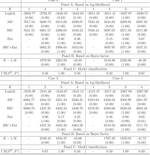
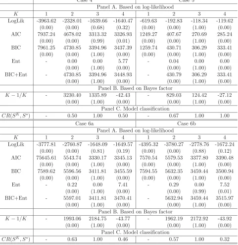
We examine the accuracy of the mixture multiple change-point model approach in grouping the simulated data set of pairs of specific turning point dates in the correct number of clusters in Table 1. For this purpose, we estimate a set of models MK forK = 1, ...., K∗, withK∗ = 4, and compute the measures described in Section 2.3 for each K in each of the 1000 simulations from Case 0 to Case 6b. For each case, the first two panels of the table report the average values of the measures that determine the number of clusters over the 1000 simulations. In addition, in brackets, the table shows the ratio of the number of times that the model selection procedure chooses modelMK over the total number of simulations, which estimates the probability that the model selection procedure chooses K clusters in the mixture model.
The table shows that the measures used to determine the number of clusters unequivocally indi-cate that the synthetic reference cycle generated in this simulation contains three separate clusters of pairs of specific turning point dates for each of the cases that we consider in the simulation. For example, for Case 0, the reported average log value of the estimated marginal likelihood reaches a maximum of −1640.50 for K = 3 clusters. The averages of AIC, BIC and BIC corrected by misclassification reach their respective minimums of 3315.00, 3396.65, and 3396.65 also for K = 3 clusters.17
Continuing with Case 0, the average of the entropy associated with the model with three clusters is zero, indicating a perfect classification of the simulated specific turning points. Finally, the sequence of averaged (twice the log of) Bayes factors also points toK= 3 because the differences of the averaged BICs are well above the values that indicate strong evidence for the model with larger number of clusters for the comparisons of the models with K = 1 versus K = 2 and the models with K = 2 versus K = 3. However, increasing K from 3 to 4 clusters implies that the difference of the averaged BICs of the models withK = 3 versus K= 4 is −43.88, which decreases the averaged odds of a model withK= 4 clusters relative to a model withK = 3 clusters. Notably, regardless of the model selection procedure, the ratios reported in brackets show that the mixture model is estimated with the right number of three clusters in all the simulations.18
It is worth pointing out that, although we use Case 0 to describe the table, the accuracy of the mixture multiple change-point model approaching to determining the correct number of clusters is consistent regardless of the case being considered. For each of these cases, the model selection procedures described in this section unambiguously chooses K= 3 clusters even if long recessions, short expansions, low quality of indicators, low number of indicators, or non-coincident indicators were involved in the dating procedure.
17Note thatBIC coincides withBIC corrected by misclassification forK= 3 because, in this case, the averaged
entropy is zero.
18The only exception is the marginal likelihood, which overestimate the number of clusters 18% of the time because
this method tends to choose models with a large number of components.
which will result in skewness around these clusters of turning points. To examine the effect of departures from the symmetry implied by the Gaussian mixtures, in Cases 6a and 6b, we simulate the specific turning points from right-skewed and left-skewed distributions, respectively, by com-puting a mixture of two distributions. The first one is a normal distribution with the true mean parameters and the second one is a normal distribution that displaces the mean parameters by -3 months in Case 6a and by +3 months in Case 6b. The proportion of the two distributions is 90% and 10%, respectively.
where #
s(im)=k
counts the number of times that observationiis allocated to cluster kacross theM replications, with k= 1, . . . , K. A natural classification indicator SK =sK1 , . . . , sKN that arises from the classification probabilities of a Markov-switching mixture model withKclusters will associate each observation τi with component k, i.e. sKi =k, if P r(si =k|θ) reaches a maximum atkover the K components.
LetS∗= (s∗1, . . . , s∗N) be the true allocation of the simulated data. To measure the ability of a mixture model to assign any specific pair of turning points to thekth group with the classification indicatorSK when it actually arises from that group according to the true classification S∗, we use
whereI{sK
i =s∗i}takes the value of one whenever observationiis classified byS
K in the same cluster
as the true allocationS∗ and zero when this observation is misclassified. Evidently, an allocation
SKwith a classification rate of 1 indicates perfect classification becausesKi =s∗i for alli= 1, . . . , N. For each case, the extent to which the selection of the number of clusters in the mixture model of simulated pairs of turning point dates determines a good partition of the underlying reference date is examined in the last panel of Table 1. The table reports the average value over the 1000 simulations of the classification rate for various numbers of clusters. For example, in Case 0, when the number of clusters is under-fitted, which occurs whenK = 2, only 46% of the observations are allocated in the correct cluster. The classification rate of the model with an over-fitted number of clustersK = 4 is 0.5, indicating that about half of the observations are misclassified. Notably, the classification rate of the model that correctly uses K = 3 clusters is one, which implies that, on average, all the observations are allocated correctly.
Again, although we used Case 0 as a basis to describe the results reported in Table 1, a detailed inspection of this table reveals that all the results obtained for Case 0 are consistent for each of the cases that we consider in the simulation study. This highlights the valuable ability of the model to provide an accurate classification of the specific pairs of turning point dates into the different phases of the reference cycle even when the latter contains double dip recessions, uncertain turning points, short samples of specific turning points, and asymmetric cycles, which appear when the disaggregated economic indicators are not coincident.
3.4 Model estimation
In this section, we use the MCMC draws for each of the 1000 simulations for the analysis of the accuracy of the mixture multiple change-point model to recover the true parameters of the means and the variances of theK distributions of the mixture.
3.3 Model classification
In addition to model selection, it is worth examining the ability of the Markov-switching mixture model to provide a posterior classification of the simulated pairs of specific turning point dates into the different time partitions provided by the reference dates. For this purpose, for each of the 1000 simulations, we estimate the posterior classification probabilities from the 2000 MCMC draws by the corresponding relative frequency from the retained state draws
Pr (si =k|θ) = 1
M#
s(im) =k
, (17)
the classification rate
N
CRSK, S∗= 1
N
N
i=1
I{sK
To check for the accuracy of the model to estimate the means, the first panel of Table 2 shows the Mean Squared Errors (M SE) as the averages over the 1000 simulations of the squared differences between the posterior means and the true reference dates. Compared to the values of the true reference dates, which range from 1980 to 2000, the estimated M SE, which range from 1.50 to 10.17, indicate that the estimated parameter values tend to be very close to the true parameter values. This high precision in parameter estimation is also observed in the low M SE in the comparison of the posterior variances and the traces of the covariance matrices and their respective true values.
Notably, these accurate results are consistent regardless of the case being evaluated, even in the cases where inference about the reference cycle is computed from a reduced set of coincident indicators or from a set of low-quality indicators. However, the accuracy in recovering the true parameters diminishes a bit when the specific reference dates are computed from non-coincident indicators.
4.1 Dating the historical turning points
The set of disaggregated coincident economic indicators that we use to evaluate the method is based on the latest available decisions of the NBER Business Cycle Dating Committee about the timing of the US business cycle turning points. In its most recent memorandum explaining the June 2009 trough (NBER Business Cycle Dating Committee 2010), the Committee mentions that it pays particular attention to ten monthly indicators when determining the trough of the Great Recession in the US reference cycle.19 These indicators are a measure of monthly GDP that has been developed by the private forecasting firm Macroeconomic Advisers, three measures of monthly GDP and GDI that have been developed by Stock and Watson (2010b), real manufacturing and trade sales, industrial production, real personal income excluding transfers, the payroll and household measures of total employment, and an aggregate of hours of work in the total economy. Although the number of available observations differs across indicators due to different starting dates and different release lags, the largest sample spans the period from January 1959 to August 2010, during which there were eight complete NBER-referenced business cycles.20
The first step of the empirical illustration consists of identifying the individual chronologies of turning points in each of the ten indicators. To this end, we apply the peak and trough dating
algo-20The Great Recession of 2008 marked the last complete cycle in our sample. Therefore, no further specific turning
point is detected since then and the sample is still valid to compute historical dates.
19An Excel spreadsheet containing the data for the indicators of economic activity considered by the committee is
available at
mirror.nber.org/cycles/BCDCFiguresData100920 ver5.xls
The objective of this section is to provide an empirical assessment of the extent to which the mixture multiple change-point model described in this paper is able to compute accurate inferences about the reference business cycle turning points in an empirical example with real data. For this purpose, we focus on the comparison of chronologies of two methods of dating the US reference cycle: the NBER-referenced business cycle dates, which serves as the standard for accuracy, and the reference dates obtained from the mixture multiple change-point model.
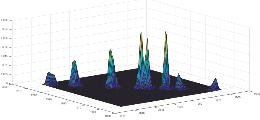
rithm code implemented by Watson (1994), who followed the lines suggested by Bry and Boschan (1971).21 Figure 1 provides a preliminary inspection of the data by plotting the kernel density estimator of the bivariate distribution of the resulting pairs of specific peaks and troughs. The figure reveals that the distribution of turning points is multimodal, exhibiting various modes that cluster the individual turning points around periods of NBER-referenced recoveries and declines. The modes of the kernel density of pairs of specific peaks and troughs suggest that the tentative number of different clusters in the reference cycle could be eight, which correspond with the distinct local maxima.
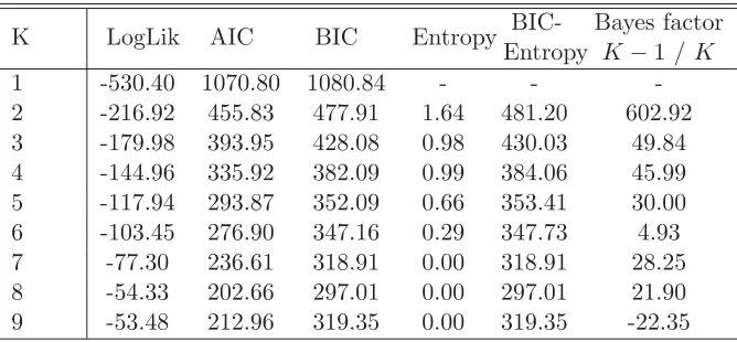
To determine the number of clusters formally, we estimate a set of models MK for K = 1, ...., K∗, with K∗ = 9, and compute the measures described in Section 2.3 for each K, whose
21In short, the algorithm isolates local minima and maxima of each of the ten indicators, subject to constraints on
both the length and amplitude of expansions and contractions.
estimates are reported in Table 3. The first column of the table shows that the log of the marginal likelihood increases uninterruptedly when the number of clusters increases from K = 1 to K = 9, where it reaches a peak at −53.48. This corresponds with K = 9, although this value is very close to that obtained for K = 8, −54.33. Although this suggests choosing K = 9, the marginal likelihood does not take into account the number of parameters in model selection and tends to overestimate the number of clusters.
Regarding model selection criteria that introduce penalties in model selection, the reported values in Table 3 of AIC, BIC and BIC corrected by misclassification reach their minimums of 202.66, 297.01, and 297.01, respectively, whenK = 8. This indicates that the US reference cycle requires eight separate cycles. In addition, the entropy of the mixture model with eight clusters is zero, showing that the model produces a clear segmentation of the reference cycle. Finally, the sequence of (twice the log of) Bayes factors that compare two models withK−1 and K different numbers of clusters, with K = 1, . . . ,9, also points to K = 8. The differences of the BICs are above the numbers favoring K in the comparison of models with K −1 versus K clusters, for
K = 1, . . . ,8. However, the difference of the BICs that compares a model with K = 9 versus a model with K−1 = 8 becomes negative (−22.25), which supports the conclusion that there is strong empirical evidence that the number of complete cycles in the US reference cycle from 1959 to 2010 is eight, as the NBER-referenced chronology establishes.
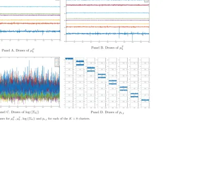
Figure 3 shows diagnostic plots of the post burn-in draws from the conditional distributions of μPk, μTk, log (|Σk|) and pk,k and pk,k+1 for each of the K = 8 clusters. These panels help us to detect potential convergence problems or label switching, which arise when the mixture likelihood function is not invariant to relabeling the components of a mixture model. The paths of the draws show that the rejection sampler that imposes, μPk(m) < μkT(m) < μPk+1(m), for all k = 1, . . . , K, is useful to prevent label switching because the sampler stays within the modal regions corresponding to the initial labeling. So, these regions are well separated from the others leading to a unique labeling.
Table 4 evaluates the mixture multiple change-point model in terms of its capacity to determine the NBER reference cycle dates. The columns labeled as NBER and MSMM report the reference
22The credible intervals, which range from 0.08 to 1.08 years for peaks and from 0.07 to 1.98 years for troughs,
provide a precise estimate of the reference dates.
23The only exception is the 2001 trough, which is located only four months after the NBER dating. The difficulties
of identifying this mild recession have been documented in Kliesen (2003) and Hamilton (2011).
24
Although the ex-post identification of the reference cycle turning points is of great interest in itself, doing this on an out-of-sample basis is a bigger challenge (Hamilton, 2011). In this section, we evaluate both the accuracy and the speed with which the mixture multiple change-point model would have dated the US reference cycle as additional specific cycle turning points were appearing in (pseudo) real time. Again, the NBER chronology is the basis of comparison.
cycle dates as determined by the NBER and our Markov-Switching Mixture Model. The distinct means are estimated from the posterior distributions with the help of the rejection Gibbs sampler algorithm for the mixture model. Using the outputs of the MCMC algorithm, this table also reports, in brackets, the range of values of the posterior probability distributions that includes 95% of the probability.22 It is evident that the mixture model replicates the NBER peak and trough dates very accurately. The method provides exact matches for one peak and three troughs, differing by less than one quarter either way in the date of the remaining turning points.23 On average, the method locates the peaks about one and a half months before and the troughs about one sixth of a month after the NBER dating. Remarkably, there are no instances in which an NBER turning point date is not matched by a similar date produced by the MSMM model, whose 95% credible intervals include the NBER-referenced dates in all the episodes.
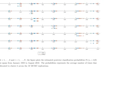
To provide the results with additional economic meaning, it is worth examining the ability of the mixture multiple change-point model to provide a posterior classification of the specific turning point dates into the different business cycles of the US reference cycle. With this aim, we estimate the posterior classification probabilities Pr (si =k|θ), with k = 1, . . . ,8 and i = 1, . . . , N, from the MCMC draws through the corresponding relative frequency of the retained state draws, as described in Section 3. Figure 4, which plots the estimated classification probabilities for each cluster, shows that the model clearly classifies each specific date, whose classification probabilities are always close to either 1 or 0. In addition, the probabilities agree with the multiple change-point behavior of the model, with a large persistence of each state and probabilities that increase nearly to unity after each structural break that occurs about the turning point dates identified by the NBER. Thus, the probabilities support the view that the mixture multiple change-point model performs a segmentation of the time span into non-overlapping business cycle episodes that agrees with the NBER-referenced cycles.
y g ( ) ( )
24Producing real-time vintages is unfeasible because the historical records of some of the ten indicators are not
available.
For this purpose, we use the same data of ten coincident economic indicators described in the in-sample analysis, which are available from 1959.01 to 2010.08. However, we develop here a pseudo real-time analysis that consists of computing inferences from successive partitions (one-month enlargements) of the latest available data set.24 In short, the new information provided by the ten economic indicators is incorporated into the model month by month as we enlarge the data set and the model converts the turning point detection into a classification problem. Each month, the model determines whether the set of incoming specific turning points dates generates a separate cluster, which would imply that a phase change occurs. To avoid false signals, we follow Chauvet and Piger (2008) and require that the Bayes factor indicates an increase in the number of clusters for 3 consecutive months, to confirm that a new reference cycle turning point has appeared. In addition, since the reference cycle dates are the means of the clusters of the specific dates, we do not date the new reference turning point until the new specific turning points appear in at least one-third of the macroeconomic indicators.25
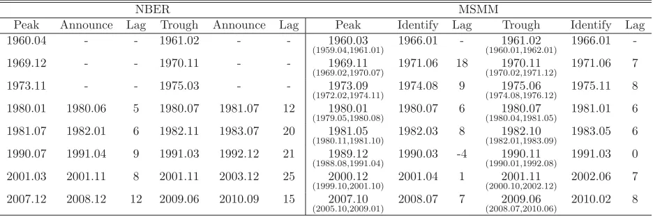
Table 5 evaluates the capacity of the mixture multiple change-point model to date the US reference cycle in pseudo real time. For a comparative assessment, the left panel reports the NBER peaks and troughs and the months of their respective announcements, while the right panel displays the estimated reference cycle turning point chronology produced by the mixture multiple change-point model and the months when the model detects the phase changes. Using the sample of the posterior draws, the table reports not only the sample means as point estimates but also the credible intervals, which are constructed using the 2.5% and 97.5% sample quantiles. Then, comparing the NBER dates with those established by MSMM measures the accuracy, while comparing the official months of the announcements with the months in which MSMM identifies the phase changes quantifies the speed of detection.
The specification whose clusters are determined by Gaussian distributions with meansμPk, μTk, the peaks and troughs of the reference cycle, is called peak-trough MSMM. On the other hand, the model that determines a reference cycle beginning with a trough and whose specific troughs and peaks are clustered around the means of bivariate Gaussians distributions μTk, μPk, is called trough-peak MSMM. The recursive analysis starts with a vintage of data that covers the period 1959.01-1966.01, which includes one pair of NBER peak-trough dates. Using this sample, we identify the specific turning points for each indicator by implementing the Bry-Boschan dating algorithm. Then, we employ the Bayes factor of the peak-trough MSMM model to confirm that there is only one cluster of specific turning point dates, which is generated from a bivariate normal density whose means are the first pair of peak-trough reference dates. According to the figures reported in Figure 5, μP1 and μT1 are dated in 1960.03 and 1961.02, respectively.
Now, the sample is enlarged by adding one month of observations to each of the ten indicators and the Bry-Boschan algorithm is re-estimated for the period 1959.01-1966.02. If the outcome of the dating algorithm does not include any new specific peak, the vintage of data is enlarged again with the observations of a new month. On the contrary, when a new specific peak is detected by the Bry-Boschan algorithm, we follow the simple automatic procedure of creating its artificial pair (trough) by adding the average duration of the preceding recessions to that peak (the preliminary
25Estimating the means with only the early available specific turning points would erroneously produce ex-ante
trough will be replaced by the actual trough as soon as it is detected by Bry-Boschan when new data arrive). In this way, we increase the sample month by month and estimate the peak-trough MSMM model with the enlarged outcomes of the Bry-Boschan algorithm. The recursive updated estimation of the first cluster stops when the Bayes factor that compares the model with K = 1 versus the model with K = 2 indicates that a new cluster has appeared. As Table 5 reports, this happens in 1971.06 and the peak μP2 is dated in 1969.11.
The procedure described above does not guarantee an accurate estimation of the trough μT2 because it could be partially based on artificial specific troughs. The approach we follow to detect the following trough is to move to the trough-peak MSMM model as soon as a new peak is detected. In this case, we omit the peak dated in 1960.03, which converts the reference cycle in a sequence of clusters centered in pairs of troughs and peaks. Then, the procedure follows the same rules described above: (i) the sample is updated by one period; (ii) the Bry-Boschan routine is used to detect new troughs, which are matched up with artificial peaks that guarantee that the current expansion will last the average of the preceding expansions (replaced by actual peaks when they appear as the outcome of the Bry-Boschan algorithm); and (iii) the peak-trough MSMM model is estimated and the Bayes factor that compares the trough-peak MSMM model with K = 1 versus the model with K = 2 is computed. The automatic procedure continues until K = 2 is preferred toK = 1, which happens in 1971.06 as reported in Table 5. At this point, we date the trough μT2 in 1970.11 and we move again to the trough-peak MSMM model with the aim of detecting a new phase change and dating the following peak μP3.
This automatic procedure goes back and forth from the peak-trough model to the trough-peak model when new turning points are detected, increasing the sample month by month and applying the classification procedure provided by MSMM to the enlarged data sets until the end of the sample in 2010.08. Table 5 examines the success of an analyst who applies MMSM to date the NBER reference cycle turning point dates in (pseudo) real time each month between 1966.01 and 2010.08, both in terms of timeliness and accuracy. Beginning with the accuracy, the dates assigned to the reference cycle turning points in pseudo real time are in close agreement to those determined by the NBER, although the precision of these estimates varies across episodes. The mixture model produces the same turning points as the NBER in one out of eight peaks and in five out of eight troughs, and are within a quarter of each other in all but one case. The noticeable exception is the peak dated in 1989.12 by our method, well before the peak dated in 1990.07 by the NBER, suggesting that this peak is associated with a leading pattern of some of the coincident indicators. It is remarkable that the credible intervals contain the NBER dates in all cases.
in the speed with which the dating methods surveyed by Hamilton (2011) identify the turning points of the Great Recession.
5
Conclusion
Since the early work of Burns and Mitchell (1946), the reference cycle is viewed as a sequence of business cycle fluctuations occurring at about the same turning points in many economic activities, where the dates of the shifts determine the reference dates. However, the fact that the cyclical turns of different processes are concentrated around certain points in time does not imply that dating the reference cycle is merely a matter of counting the economic time series that rise and that fall at about the same time. In fact, dating the reference cycle has been the source of much debate in both the research literature and policy. The approach pursued in this paper to date the reference cycle is based on aggregating the specific turning points from a set of coincident economic indicators.
In our novel proposal, the set of specific turning points dated from a set of coincident indicators is viewed as a sequence of data with a natural ordering which can be broken down into segments by the reference cycle turning points. In particular, the specific turning points are supposed to be drawn from the same Gaussian distribution within each segment, but from different Gaussian distributions in different segments. Thus, the set of bivariate individual turning points are con-sidered to arise from a mixture distribution where the different model parameters are assumed to evolve according to a latent random discrete-state Markov process with the transition probabilities constrained as in the multiple-change break point model proposed by Chib (1998). In this repre-sentation, the means of the different Gaussian distributions are viewed as natural estimates of the reference cycle turning points and the state probabilities are used to determine the change points of the different reference cycles and to classify the specific turning point dates into the different business cycles of the reference cycle. In this context, standard Bayesian estimation of finite Markov mixture modeling techniques is suggested to estimate the model.
The reliability of the proposed framework is validated with simulated data in a Monte Carlo experiment that try to mimic some stylized facts of business cycle analyses such as short business cycle phases, uncertain turning points, short samples and specific cycles that come from non-coincident indicators. The results suggest that the method is very accurate to determine the number of clusters, to classify the set of specific turning points and to recover the true parameters, regardless of the stylized business cycle fact being analyzed.