M E T H O D O L O G Y A R T I C L E
Open Access
A probabilistic algorithm to process
geolocation data
Benjamin Merkel
1,2*, Richard A. Phillips
3, Sébastien Descamps
1, Nigel G. Yoccoz
2, Børge Moe
4and Hallvard Strøm
1Abstract
Background:The use of light level loggers (geolocators) to understand movements and distributions in terrestrial and marine vertebrates, particularly during the non-breeding period, has increased dramatically in recent years. However, inferring positions from light data is not straightforward, often relies on assumptions that are difficult to test, or includes an element of subjectivity.
Results:We present an intuitive framework to compute locations from twilight events collected by geolocators from different manufacturers. The procedure uses an iterative forward step selection, weighting each possible position using a set of parameters that can be specifically selected for each analysis.
The approach was tested on data from two wide-ranging seabird species - black-browed albatrossThalassarche melanophrisand wandering albatrossDiomedea exulans–tracked at Bird Island, South Georgia, during the two most contrasting periods of the year in terms of light regimes (solstice and equinox). Using additional information on travel speed, sea surface temperature and land avoidance, our approach was considerably more accurate than the traditional threshold method (errors reduced to medians of 185 km and 145 km for solstice and equinox periods, respectively). Conclusions:The algorithm computes stable results with uncertainty estimates, including around the equinoxes, and does not require calibration of solar angles. Accuracy can be increased by assimilating information on travel speed and behaviour, as well as environmental data. This framework is available through the open source R packageprobGLS, and can be applied in a wide range of biologging studies.
Keywords:Animal tracking, Global Location Sensors, GLS, Method assessment, Sea surface temperature, Probability sampling,probGLS, Threshold method
Background
The ability to track animals across large distances in space and time has revolutionized our understanding of their movements during the breeding and nonbreeding seasons [1, 2]. Thanks to the development of light-level data loggers (geolocators; also termed Global Location Sensor or GLS loggers) [3], we are now able to track small animals which cannot carry heavy satellite-transmitters or GPS (‘global positioning system’) loggers (e.g. [4, 5]). Indeed, geolocators are used very frequently on nonbreeding seabirds, because long-term deployment
of satellite or GPS devices using harnesses is a major welfare concern (e.g. [6]) and also on other marine or-ganisms, including fish, that rarely, if ever, are at the sea surface and so cannot be tracked using radio wave tech-nology. Currently, miniaturized GPS loggers in the same weight range as geolocators record few locations throughout the deployment period; thus, the data are unsuitable for answering ecological questions on finer temporal scales.
Geolocators record ambient light intensities and elapsed time, from which longitude and latitude can be estimated [3, 7]. They can record data for up to a year or longer, and cover one or several annual migration cy-cles [8, 9]. Their small size and mass (to <1 g) allow a wide range of species to be tracked, and because of the relatively low cost (compared with miniaturized GPS
* Correspondence:[email protected] 1
Norwegian Polar Institute, Fram Centre, P.O. Box 6606 Langnes, NO-9296 Tromsø, Norway
2Department of Arctic and Marine Biology, UiT The Arctic University of
Norway, NO-9037 Tromsø, Norway
Full list of author information is available at the end of the article
© The Author(s). 2016Open AccessThis article is distributed under the terms of the Creative Commons Attribution 4.0 International License (http://creativecommons.org/licenses/by/4.0/), which permits unrestricted use, distribution, and reproduction in any medium, provided you give appropriate credit to the original author(s) and the source, provide a link to the Creative Commons license, and indicate if changes were made. The Creative Commons Public Domain Dedication waiver (http://creativecommons.org/publicdomain/zero/1.0/) applies to the data made available in this article, unless otherwise stated.
Merkelet al. Movement Ecology (2016) 4:26
devices), they can be used to track many individuals for multi-population studies (e.g. [10–13]).
A number of methods have been developed to esti-mate locations from light data (Table 1), and to filter the resulting outputs in various ways [14–17]. These are mainly based on either a threshold [7, 18] or template-fit approach [19]. In the former, longitude is computed from the timing of local noon, and latitude from day length, based on the timing of twilight events (i.e. dusk and dawn) which are determined using a pre-defined light intensity threshold. Further, latitude depends on the solar angle below the horizon at which the threshold is crossed [7]. This sun elevation angle, which is affected by shading during the twilight period (related to behav-iour and activity patterns as well as weather), and lati-tude [20], has to be calibrated, and for practical purposes, is generally assumed to stay constant during the entire deployment period. In contrast, the template-fit method involves template-fitting a simplified geophysical model for various latitudes (i.e. the template) to recorded light intensities for each day at a longitude estimated in the same way as in the threshold method [21].
Unlike other tracking methods, locations derived from light data lack a constant spatial error structure. Lati-tudes are most accurate (i.e. least affected by shading) where the timing of twilight events is most distinct, i.e., during solstices and at high latitudes [7]. However, within the Arctic or Antarctic circles, position estimates are impossible around the solstices due to the lack of twilight events (i.e. polar night and midnight sun). In contrast, the error in latitude (due to shading) is highest during the equinoxes where day length is the same around the globe, and around the equator where there is little variation in day length [7].
Given the wide range of alternative methods and po-tential observer-specific biases, there would clearly be advantages in determining a common method for ana-lysing all geolocation data. Any method that requires raw light values and not just timing of twilight events (Table 1) cannot be applied to data from all brands of geolocators. For instance, Lotek geolocators (Lotek Wireless Inc., Ontario, Canada) do not store these data by default and have been deployed in many studies of marine organisms. The aim of this paper is to propose an intuitive, probabilistic algorithm, implemented in R [22] through the new package probGLS, that can be used on data from all existing geolocator brands. Our method is relatively simple, easy to implement, fast to compute (compared to other more complex methods), does not require the use of a constant solar angle (as needed in theGeoLightpackage [23]), provides uncer-tainty estimates, can incorporate additional information to increase accuracy (e.g. land avoidance for marine or-ganisms), and greatly reduces location error around the
equinoxes (if additional information is available) without making assumptions about behavioural states as in state space models (SSM, e.g. [24–27]). Here we validate the approach for two open landscape species (flying sea-birds), but its usability would need to be confirmed for other organisms, particular those that dive or live in closed terrestrial habitats (e.g. forests).
Methods Method principle
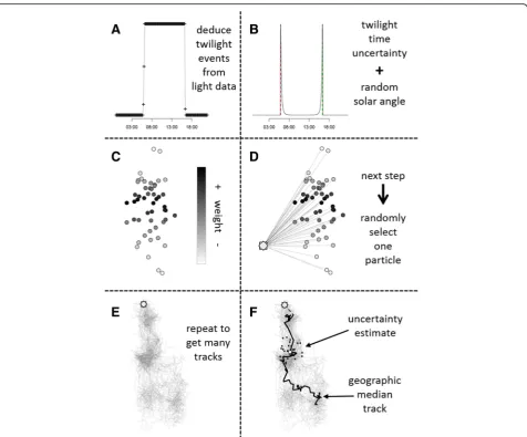
The method is an iterative forward step selection based on [28]. The algorithm uses twilight events (Panel A, Fig. 1) identified using a range of brand-specific software for analysing light data (e.g. TransEdit2, British Antarctic Survey (BAS), Cambridge, UK), the twilightCalc
function (GeoLight package; also incorporated into IntiProc, Migrate Technology, Cambridge, UK), or in the case of Lotek loggers by back-calculating twilight thresh-olds from computed locations as implemented in the
lotek_to_dataframe function (probGLS package, this study). The framework can incorporate various sources of uncertainty (e.g. uncertainty in solar angle) as well as knowledge of the behaviour and habitat use of the study species (e.g. travel speed), by defining associ-ated parameter values a priori (Table 3). The main steps are described below:
1. The algorithm assumes that the first position at time
t1is known without error (i.e. release location),
regardless of the time difference betweent1and the
first twilight event.
2. The next available pair of twilight events (dusk/dawn or dawn/dusk) is replicated x times with an
additional twilight error term (from a log-normal distributionN, μ and σ on the log scale = user-defined, See Additional file 1 for information about setting these parameters) and a random solar angle (from a user-defined range) applied to each twilight before a location is calculated (Panel B, Fig.1).
3. Using the threshold method and the twilight events computed in step 2, a cloud of positions (i.e. particles) attiis calculated. To make computations more robust, all particles outside a defined boundary box (based on known range) are removed. Further, latitudes are unreliable for a variable period around the equinoxes. For these periods (user-defined), random latitudes (with uniform distribution) within the boundary box are added to each computed longitude estimate.
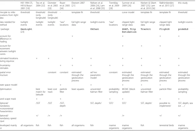
Table 1Comparison of available methods to process geolocation data Hill 1994 [7],
Hill & Braun 2001 [18]
Teo et al. 2004 [32]
Domeier et al. 2005 [33]
Royer et al. 2005 [34]
Ekstrom 2007 [21]
Nielsen et al. 2006 [24], Lam et al. 2008 [35]
Tremblay et al. 2009 [28]
Sumner et al. 2009 [26]
Nielsen & Sibert 2007 [25], Lam et al. 2010 [36]
Rakhimberdiev et al. 2015 [27]
this study
Principle to infer locations from light data threshold threshold (only longitude) threshold (only longitude)
- template fit threshold - curve model template fit template fit threshold
Data needed for method twilight events twilight events twilight events
“raw” locations
full light range data
twilight events “raw” locations
clipped light range data
full light range data
clipped light range data
twilight events
R package GeoLight [23]
Ukfsst SGAT, Trip
Estimation
Trackit FlightR probGLS
Account for difference in shading + + + + Account for movement between twilight events + + + Estimated locations during equinox + + + + + + + + Uncertainty estimates + + + + + + + + Spatial error structure
constant constant estimated through the geolocation process ad hoc parametric model constant estimated through the geolocation process estimated through the geolocation process estimated through the geolocation process estimated through the geolocation process
State space model + + + + +
Optimisation best match for latitude least cost track particle filter
least squares unscented Kalman filter probability sampling MCMC (block update) unscented Kalman filter
particle filter probability sampling
Land scape mask + + + + + +
Optional/ mandatory environmental characteristics
/SST /SST /SST, depth
SST, depth/ SST/ SST/ SST, depth/ possible to implement/
SST, depth, sea ice…/
Optional/ mandatory speed input +/ /+ /+ /+ +/ +/ Developed mainly for
all organisms fish fish fish all organisms fish marine organisms
marine organisms
5. Then, one particle is randomly selected following a distribution based on the assigned weights (Panel D, Fig.1). If all particles in a given cloud have a weight of 0, the entire cloud is considered unlikely and discarded.
6. The algorithm moves one time step forward toti+1 and steps 2 to 5 are repeated untiltn(nbeing the last set of twilight events).
7. Steps 1 to 6 are iterated a set number of times to construct several probable movement paths (Panel E, Fig.1).
8. The most likely movement path is computed as the geographic median (Additional file2) for each computed location cloud; the variation in positions
of all computed paths denotes the uncertainty at each step in time (Panel F, Fig.1).
Tremblay et al. [28] defined their particle clouds based on “raw” locations as the geographic average with a spatial error structure. This is the case for locations de-rived using satellite-transmitters. However, locations es-timated from light data using the threshold method can only be assumed to be the geographic average if the cor-rect solar angle for each day is selected, shading was similar both at dawn and dusk, and the animal only moved a short distance between twilight events. If any of these conditions is violated the position could be strongly biased. Therefore, we based our method on the
timing of twilight events, incorporating uncertainty and unknown solar angle (steps 2 & 3). This allows uncer-tainties to be incorporated that are related to differences in behaviour and weather patterns, as well as dynamic latitudinal uncertainty, which reflects the season and latitude-specific uncertainty of the geolocation method. Uncertainty in twilight events is assumed to follow a log-normal distribution. This skewed distribution takes into account that a sunrise may falsely appear to occur later, due to shading, while it is improbable that light is falsely detected prior to sunrise (and the inverse is true for sunsets). The error parameters for this uncertainty can be
generated using twilight_error_estimation
(package probGLS, this study). It is important that the error distribution mirrors the actual behaviour of the ani-mal. This should be done using calibration data (i.e. ~2 weeks of data recorded on the individual at a known location). Solar angles do not have to be calibrated or as-sumed to be constant, but rather a reasonable range of possible angles can be defined (step 2). Also, due to the above mentioned pitfalls regarding use of“raw”locations and unknown latitude and time specific error distribu-tions, we do not interpolate between positions to utilize the higher frequency of temperature measurements by the loggers as described by [28]. Steps 4 to 8 are in principle equivalent to [28]. However, we do not include weighted distributions of individual speeds computed using the next x particles in the record, but rather use a defined speed distribution. This is because there are no specific locations on which to base these distributions; instead, there is a cloud of possible locations. Moreover, we do not consider the geographic average track to be the most probable track, but the geographic median defined as the position with the minimum sum of all distances to all other iter-ated locations. Therefore the selected position will always be a computed location. In contrast, the average geo-graphic position might, for example, be on land if the cloud of points is around a land mass, even if this is un-realistic for the study species (Additional file 2).
Method assessment
The framework was tested using data from black-browed (Thalassarche melanophris) and wandering (Diomedea exulans) albatrosses (Table 2) tracked in December-January (incubation) and March-April (brood-guard), respectively, in 2015 from Bird Island, South Georgia (54°00’S, 38°03’W). All individuals were
equipped with an i-gotU GPS logger (Mobile Action Technology Inc., New Taipei City, Taiwan) taped to back feathers and programmed to log a position every 10 min, and an Intigeo C250 geolocator (Migrate Technology Ltd, Cambridge, UK) attached by cable-tie to a plastic leg ring, which measured light in the range 1.1 to 74418 lux (maximum recorded at 5 min intervals) and temperature every 20 min of continuous wet (maximum, minimum and mean saved every 4 h), and tested for salt-water immersion every 6 s.
Twilight events from raw light intensities were com-puted with twilightCalc (light threshold of 2; log-gers calibrated on Bird Island). To increase precision we included sea surface temperature (SST) and land avoid-ance. The daily median water temperature encountered by each bird was computed from temperature data col-lected every 4 h by the loggers. The daily mean satellite-derived SST and mean SST error was extracted from the NOAA optimally-interpolated, high resolution SST data-set at 0.25° resolution [29]. Each movement path incor-porated parameter values based on the ecology of the species and information extracted from GPS data (Table 3, and Additional file 3).
To compare GPS tracks to locations estimated from geolocator data, we calculated the average GPS loca-tion between two twilight events. Devialoca-tion for each geographic median, and nearest location (both derived from geolocator data) from the average GPS positions was computed as the great-circle distance [14]. Add-itionally, each average GPS position was compared to locations estimated using the classical threshold method with a fixed solar angle of -5.0° and -5.8° for black-browed and wandering albatross data, respect-ively. These angles give the smallest average deviation of the estimated locations from the corresponding average GPS location in a range of -1° to -7°. In addition, all positions outside the boundary box were removed (Table 2). Finally, we ran sensitivity analyses to assess how many particles (1 – 10 000) and track iterations (1 – 200) were necessary to obtain a stable and reliable track output (see R script in Additional file 4) as well as how changes in the uncertainty dis-tribution of twilight events changes accuracy.
Results
Combined geolocator and GPS data were obtained for 33 and 27 black-browed and wandering albatrosses,
Table 2Summary of tracking data available for method assessment
Species # of
individuals
# of tracks
mean ± sd (min–max) trip duration [days]
mean ± sd (min–max)
# of locations per track
Deployment period
black-browed albatross 33 33 9 ± 4 (3–17) 15 ± 7 (5–31) 10 Dec 2014 to 6 Jan 2015
wandering albatross 27 32 3 ± 1 (1–7) 4 ± 2 (2–9) 14 Mar 2015 to 3 Apr 2015
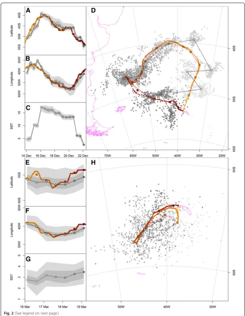
respectively, in two contrasting periods characterized by minimal (solstice) and maximal (equinox) uncertainty in latitude estimation using light data (Table 2). Examples for a black-browed albatross track during the summer solstice and a wandering albatross track during the fall equinox showing both processed geolocator and GPS lo-cations are illustrated in Fig. 2. The overall median dis-tance between the most probable geolocator and mean GPS locations was 185 km (range 5 to 2740 km) and 145 km (range 8 to 493 km) for tracks during the summer solstice and fall equinox, respect-ively (Table 4, Additional file 5). The median closest distance of each iterated location cloud to the mean GPS location was 19 km and 17 km during the sum-mer solstice and fall equinox, respectively. Using the threshold approach with a constant solar angle of -5.0° and -5.8° resulted in median distances to average GPS locations of 226 km (22% lower accuracy than the new method) and 662 km (357% lower accuracy) for the black-browed albatross data during the sum-mer solstice and wandering albatross data during the fall equinox, respectively. Moreover, only 54% of posi-tions could be calculated using the threshold method with the GeoLight package and a constant angle of -5.8° during the fall equinox compared to our new approach (Table 3).
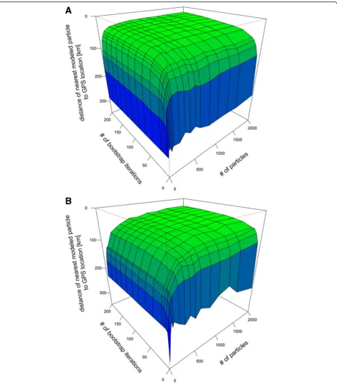
The relationship between number of particles used, number of iterations and median minimum distance of each point cloud to the average GPS locations for both time periods is illustrated in Fig. 3. Accuracy increases with increasing iterations and particles numbers, reach-ing an asymptote at around 60 iterations, and 300 and 800 particles during the solstice and equinox periods, re-spectively. Varying the shape parameter (μ) for the as-sumed twilight uncertainty distribution for both twilight events simultaneously from 1 to 4 and thereby increas-ing the possible range of error from ~8 min to ~2 h, while keeping the maximum probability at the input twi-light timing, did not seem to affect the accuracy of the results for either time period (Additional file 6).
Discussion
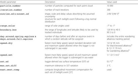
By comparing locations calculated from light and temperature data to concurrent GPS positions during two contrasting times of the year (close to the solstice and equinox), we demonstrated that our new method provides consistently high accuracy throughout the year, similar to the minimum uncertainty of the standard threshold method (i.e. during solstices at high latitudes; Table 4) [14, 30]. Tracks from two fast moving seabird species, black-browed and wandering albatrosses, could be reconstructed using this approach by incorporating Table 3Algorithm parameters used to compute locations for both assessment data sets
Model parameter Description Value used
particle.number number of particles computed for each point cloud 10 000
iteration.number number of track iterations 200
sunrise.sd & sunset.sd shape, scale and delay values describing the assumed uncertainty
structure for each twilight event following a log normal distribution
2.49/ 0.94/ 0a
range.solar range of solar angles used -7° to -1°
boundary.box the range of longitudes and latitudes likely to be used by tracked individuals
120 W to 40 E 90 S to 0
day.around.spring.equinox & days.around.fall.equinox
number of days before and after an equinox event in which a random latitude will be assigned
includes the entire wandering albatross tracking period
speed.dry fastest most likely speed, speed standard deviation (sd) and maximum speed allowed when the logger is not submerged in sea water
12/ 6/ 45 m/s
for black-browed albatrossb & 12/ 7/ 70 m/s
for wandering albatrossb
speed.wet fastest most likely speed, speed sd and maximum speed allowed when the logger is submerged in sea water
1/ 1.3/ 5 m/sc
sst.sd logger-derived sea surface temperature (SST) sd 0.5 °Cd
max.sst.diff maximum tolerance in SST variation 3 °C
east.west.comp compute longitudinal movement compensation for each set of twilight event [37]
used
a
The resulting uncertainty structure for both twilight events is illustrated in Additional file1. These parameters are chosen as they resemble the twilight error structure of open habitat species in [20]
b
inferred from GPS tracks (see Additional file3for details)
c
Antarctic circumpolar current speed up to fast current speeds (i.e. Malvinas current) [38] as the tagged animal is assumed to not actively move when the logger is immerged in seawater
d
Fig. 2(See legend on next page.)
additional environmental data (notably SST). In addition to providing positions around the equinox, this method provides an uncertainty associated with each computed position. This uncertainty could be used, for example, to build more realistic models of the measurement compo-nent of SSM for further behavioural analysis to account for the complex error structure of geolocations.
Our method for estimating locations from light-level data offers a simple, fast and intuitive approach access-ible via the R package probGLS. This method is not Baysian or based on Kalman filter in contrast to the other statistically-advanced methods that are currently available (such as the R packagesTrackit[25],SGAT/ tripEstimation [26], and FlightR [27], Table 1) and we hope it will be less of a “black box” for many ecologists, with assumptions being more transparent at the expense of a mathematically rigorous framework. As with FlightR, our method generates a cloud of pos-sible particles for each location, but uses probability sampling to construct a path rather than a particle filter. Further, the current implementation of probGLS takes about 30 min for a 1 year track (2000 particles, 100 iter-ations; Intel Core i7-3540 M 3 GHz, 16 GB RAM). This is to our knowledge faster than any SSM method (Table 1). With a run time per track of less than an hour it is feasible to run sensitivity analyses on input parame-ters (as in this study). Unlike the R packages based on SSM, probGLS cannot account for movement of the study animal between consecutive twilight events, which can reduce certainty in location estimation for certain taxa. However, it does not require the assumption or calibration of a constant solar angle throughout the year
[20, 31], unlike the classical threshold method. The rea-son is that the added uncertainty around each twilight event as well as the range of solar angles accounts for different behaviour and levels of sensor shading around sunrise and sunset during the tracking period.
Twilight events for both albatross species computed by twilightCalc were not inspected manually for false or low-confidence transitions (reflecting interrup-tions to light records), and only outliers outside the de-fined boundary box (Table 3) were removed during processing. The range in accuracy, in particular for black-browed albatross data (Table 4), shows that the method was unable to correct twilight events which are far from the correct time (i.e. falsely assigned). These re-sult in unreliable location clouds which the algorithm will attempt to fit into the movement path. However, most of these outliers were removed subsequently in the algorithm based on the assumed speed distribution, as well as land avoidance and SST weighting (steps 4 & 5). Accuracy could be improved if twilight events are either
edited manually, filters such as loessFilter
(GeoLight package) are applied, or the extent of the boundary box reduced before running the new method.
The number of particles needed for computation depends on the range of latitudes set in the param-eter boundary.box (i.e. assumed latitudinal range during the equinox) as well as the longitudes defined
through the parameters sunrise.sd and
sunset.sd. We let latitude during the equinox vary by 90° (Table 3) as we did not expect the tracked in-dividuals to cross the equator, whereas longitudinal uncertainty was assumed to vary over ~35 min to (See figure on previous page.)
Fig. 2Examples trips from a black-browed albatross during the summer solstice (a-d) and a wandering albatross during the fall equinox (e-h). (a toc & etog) show the change in latitude, longitude and encountered sea surface temperature (SST) with time while (d & h) represent the tracks. Grey scale positions show all processed geolocator locations; black framed grey positions represent median geographic geolocator locations; red symbols represent 10 min resolution GPS locations; black framed red squares are daily average GPS locations; track direction from light to dark. Shaded grey areas in (a) to (c) represents 95 and 50% uncertainty
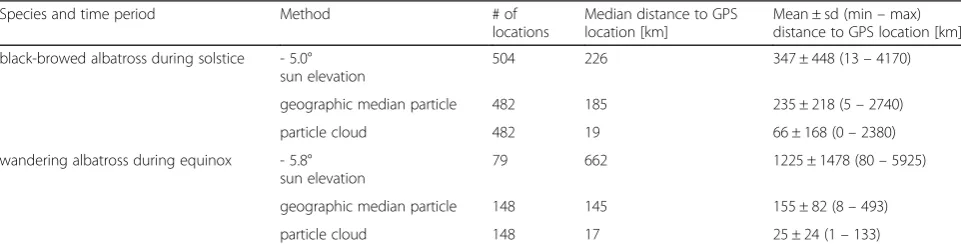
Table 4Summary of number of locations estimated and distance to average GPS position using two methods of light level location estimation
Species and time period Method # of locations
Median distance to GPS location [km]
Mean ± sd (min–max) distance to GPS location [km]
black-browed albatross during solstice - 5.0° sun elevation
504 226 347 ± 448 (13–4170)
geographic median particle 482 185 235 ± 218 (5–2740)
particle cloud 482 19 66 ± 168 (0–2380)
wandering albatross during equinox - 5.8° sun elevation
79 662 1225 ± 1478 (80–5925)
geographic median particle 148 145 155 ± 82 (8–493)
particle cloud 148 17 25 ± 24 (1–133)
account for differences in shading due to behaviour and weather patterns (Table 3, Additional file 1). Based on Fig. 3, at least 800 particles are needed for stable results throughout the year. If the latitudinal uncertainty during the equinox is 180° (i.e. from pole to pole) the number of particles would need to be
doubled. The minimum number of iterations needed for a consistent output was already reached at 60.
The median closest distance of each iterated location cloud to the mean GPS location of 19 and 17 km in the two time periods (Table 4) reflects the 0.25° spatial reso-lution of the satellite-derived SST dataset. Using a higher
Fig. 3Median distance between the nearest particle and its associated average GPS location in relation to number of iterations and number of particles used.aBlack-browed albatross data during the summer solstice;bWandering albatross data during the fall equinox
resolution SST dataset will likely increase the accuracy of this approach for this particular example. This illus-trates that the selected weightings, as well as their reso-lution influence the accuracy and degree of uncertainty of a track. A high range of solar angles, a high uncer-tainty in twilight events and high assumed movement speed, combined with a lack of available environmental characteristics will lead to greater uncertainty and lower accuracy overall. Conversely, the accuracy of the method would increase if the range of solar angles as well as the twilight event uncertainty could be restricted based on previous knowledge (e.g. calibration periods).
We have demonstrated here that the algorithm achieves stable results with fast moving species in open landscapes (flying seabirds) and are optimistic that re-sults would be comparable for animals inhabiting other habitats (e.g. terrestrial birds and diving organisms), es-pecially if additional information to weight the com-puted particles is available. We already have preliminary indications that the algorithm performs well on diving species such as penguins. However, the suitability of the method for a wider range of species has to be confirmed in further studies.
Conclusion
We presented an intuitive and time-efficient algorithm which makes it possible to analyse geolocator data from loggers of different types and manufacturers, deployed on any animal, throughout the year, including equinox periods (if sufficient additional information is available), in a consistent way, while acknowledging the limitations and uncertainties associated with light data. We do not claim that it is the most accurate method, but rather that it can be used widely and easily, regardless of whether the data were processed using outmoded software or new methods, without requiring a subjective step in determining or filtering locations.
Additional files
Additional file 1:Twilight event uncertainty structure. (PDF 362 kb)
Additional file 2:Geographic median description. (PDF 205 kb)
Additional file 3:Recorded ground speed frequencies. (PDF 246 kb)
Additional file 4:R script for sensitivity analyses. (TXT 9 kb)
Additional file 5:Histograms of deviation of GLS computed locations to average GPS locations using two methods of light level location estimation. (PDF 257 kb)
Additional file 6:Sensitivity analysis for changing shape parameters determining the twilight event uncertainty. (PDF 308 kb)
Abbreviations
GLS:Global location sensor; GPS: Global positioning system; SSM: State space model; SST: Sea surface temperature
Acknowledgements
We are grateful to Karen Lone, Simeon Lisovski, Vegard Bråthen and Halfdan H. Helgason for comments on the method and early drafts, and to Jessica Walkup and Lucy Quinn for assistance with fieldwork at Bird Island. Further, we would like to thank two anonymous reviewers whose comments helped to improve the manuscript considerably.
Funding
The study was financed by the Norwegian SEATRACK programme which is funded by the Norwegian Ministry of Climate and Environment, Ministry of Foreign Affairs and the Norwegian Oil and Gas Association along with seven oil companies (Statoil Petroleum AS, Det norske oljeselskap ASA, Eni Norge AS, Total E&P Norge AS, ConocoPhillips Skandinavia AS, Engie and DEA Norge AS).
Availability of data
The source code for the probGLS R package as well as an example workflow for several logger manufacturers is available on GitHub: https://github.com/ benjamin-merkel/probGLS.
Authors’contributions
BMe conceived the study. BMe, RP, NY and SD developed the detailed method. BMe coded the R package. BMe wrote the first draft of the manuscript, with contributions from RP, SD, NY, BMo and HS. All authors read and approved the final manuscript.
Competing interests
The authors declare that they have no competing interests.
Consent for publication Not applicable.
Ethics approval and consent to participate
All fieldwork was approved by the British Antarctic Survey Ethics Committee and carried out under permit from the Govt. of South Georgia and the South Sandwich Islands.
Author details
1Norwegian Polar Institute, Fram Centre, P.O. Box 6606 Langnes, NO-9296
Tromsø, Norway.2Department of Arctic and Marine Biology, UiT The Arctic
University of Norway, NO-9037 Tromsø, Norway.3British Antarctic Survey,
Natural Environment Research Council, High Cross, Madingley Road, Cambridge CB3 0ET, UK.4Norwegian Institute for Nature Research, P.O. Box
5685Sluppen, NO-7485 Trondheim, Norway.
Received: 2 May 2016 Accepted: 4 November 2016
References
1. Block BA, Jonsen ID, Jorgensen SJ, Winship AJ, Shaffer SA, Bograd SJ, Hazen EL, Foley DG, Breed GA, Harrison AL, et al. Tracking apex marine predator movements in a dynamic ocean. Nature. 2011;475:86–90.
2. Bowlin MS, Bisson I-A, Shamoun-Baranes J, Reichard JD, Sapir N, Marra PP, Kunz TH, Wilcove DS, Hedenström A, Guglielmo CG, et al. Grand Challenges in Migration Biology. Integr Comp Biol. 2010;50:261–79.
3. Wilson RP, Ducamp J-J, Rees WG, Culik BM, Niekamp K. Estimation of location: global coverage using light intensity. In: Priede IG, Swift SM, editors. Wildlife telemetry - Remote Monitoring and Tracking of Animals. England: Ellis Horwood; 1992. p. 131–4.
4. Egevang C, Stenhouse IJ, Phillips RA, Petersen A, Fox JW, Silk JRD. Tracking of Arctic terns Sterna paradisaea reveals longest animal migration. Proc Natl Acad Sci. 2010;107:2078–81.
5. Stutchbury BJM, Tarof SA, Done T, Gow E, Kramer PM, Tautin J, Fox JW, Afanasyev V. Tracking Long-Distance Songbird Migration by Using Geolocators. Science. 2009;323:896.
7. Hill RD: Theory of geolocation by light levels. In Elephant seals: population biology, behavior, and physiology (Le Boeuf BJ, Laws RM eds.). Berkely, CA, USA.: Univ. California Press.; 1994:pp. 227-236.
8. Croxall JP, Silk JRD, Phillips RA, Afanasyev V, Briggs DR. Global Circumnavigations: Tracking Year-Round Ranges of Nonbreeding Albatrosses. Science. 2005;307:249–50.
9. Weimerskirch H, Wilson RP. Oceanic respite for wandering albatrosses. Nature. 2000;406:955–6.
10. Frederiksen M, Moe B, Daunt F, Phillips RA, Barrett RT, Bogdanova MI, Boulinier T, Chardine JW, Chastel O, Chivers LS, et al. Multicolony tracking reveals the winter distribution of a pelagic seabird on an ocean basin scale. Divers Distrib. 2012;18:530–42.
11. Tranquilla LAM, Montevecchi WA, Hedd A, Fifield DA, Burke CM, Smith PA, Regular PM, Robertson GJ, Gaston AJ, Phillips RA. Multiple-colony winter habitat use by murres Uria spp. in the Northwest Atlantic Ocean: implications for marine risk assessment. Mar Ecol Prog Ser. 2013;472:287–303.
12. Fort J, Pettex E, Tremblay Y, Lorentsen S-H, Garthe S, Votier S, Pons JB, Siorat F, Furness RW, Grecian WJ, et al. Meta-population evidence of oriented chain migration in northern gannets (Morus bassanus). Front Ecol Environ. 2012;10:237–42.
13. Ramos R, Sanz V, Militão T, Bried J, Neves VC, Biscoito M, Phillips RA, Zino F, González-Solís J. Leapfrog migration and habitat preferences of a small oceanic seabird, Bulwer’s petrel (Bulweria bulwerii). J Biogeogr. 2015;42:1651–64.
14. Phillips RA, Silk JRD, Croxall JP, Afanasyev V, Briggs DR. Accuracy of geolocation estimates for flying seabirds. Mar Ecol Prog Ser. 2004;266:265–72.
15. Guilford T, Meade J, Willis J, Phillips RA, Boyle D, Roberts S, Collett M, Freeman R, Perrins CM. Migration and stopover in a small pelagic seabird, the Manx shearwater Puffinus puffinus: insights from machine learning. Proc R Soc Lond B Biol Sci. 2009;276:1215–23.
16. Mosbech A, Johansen K, Bech N, Lyngs P, Harding AA, Egevang C, Phillips R, Fort J. Inter-breeding movements of little auks Alle alle reveal a key post-breeding staging area in the Greenland Sea. Polar Biol. 2012;35:305–11. 17. Hanssen SA, Gabrielsen GW, Bustnes JO, Bråthen VS, Skottene E, Fenstad AA,
Strøm H, Bakken V, Phillips RA, Moe B: Migration strategies of common eiders from Svalbard: Implications for bilateral conservation management. Polar Biol. 2016;39(10):1–10.
18. Hill R, Braun M: Geolocation by Light Level. In Electronic Tagging and Tracking in Marine Fisheries. Volume 1. Edited by Sibert J, Nielsen J: Springer Netherlands; 2001: 315–330: Reviews: Methods and Technologies in Fish Biology and Fisheries].
19. Ekstrom P. An advance in geolocation by light. Memoirs National Ins Polar Res Special Issue. 2004;58:210–26.
20. Lisovski S, Hewson CM, Klaassen RHG, Korner-Nievergelt F, Kristensen MW, Hahn S. Geolocation by light: accuracy and precision affected by environmental factors. Methods Ecol Evol. 2012;3:603–12.
21. Ekstrom P. Error measures for template-fit geolocation based on light. Deep-Sea Res II Top Stud Oceanogr. 2007;54:392–403.
22. R Development Core Team. R: A language and environment for statistical computing. Vienna, Austria: R Foundation for Statistical Computing; 2016. 23. Lisovski S, Hahn S. GeoLight–processing and analysing light-based
geolocator data in R. Methods Ecol Evol. 2012;3:1055–9.
24. Nielsen A, Bigelow KA, Musyl MK, Sibert JR. Improving light-based geolocation by including sea surface temperature. Fish Oceanogr. 2006;15:314–25.
25. Nielsen A, Sibert JR. State–space model for light-based tracking of marine animals. Can J Fish Aquat Sci. 2007;64:1055–68.
26. Sumner MD, Wotherspoon SJ, Hindell MA. Bayesian Estimation of Animal Movement from Archival and Satellite Tags. PLoS One. 2009;4:e7324. 27. Rakhimberdiev E, Winkler D, Bridge E, Seavy N, Sheldon D, Piersma T,
Saveliev A. A hidden Markov model for reconstructing animal paths from solar geolocation loggers using templates for light intensity. Movement Ecol. 2015;3:25.
28. Tremblay Y, Robinson PW, Costa DP. A Parsimonious Approach to Modeling Animal Movement Data. Plos One. 2009;4:e4711.
29. Reynolds RW, Smith TM, Liu C, Chelton DB, Casey KS, Schlax MG. Daily High-Resolution-Blended Analyses for Sea Surface Temperature. J Clim. 2007;20:5473–96.
30. Shaffer S, Tremblay Y, Awkerman J, Henry RW, Teo SH, Anderson D, Croll D, Block B, Costa D. Comparison of light- and SST-based geolocation with satellite telemetry in free-ranging albatrosses. Mar Biol. 2005;147:833–43.
31. Fudickar AM, Wikelski M, Partecke J. Tracking migratory songbirds: accuracy of light-level loggers (geolocators) in forest habitats. Methods Ecol Evol. 2012;3:47–52.
32. Teo SLH, Boustany A, Blackwell S, Walli A, Weng KC, Block BA. Validation of geolocation estimates based on light level and sea surface temperature from electronic tags. Mar Ecol Prog Ser. 2004;283:81–98.
33. Domeier ML, Kiefer D, Nasby-Lucas N, Wagschal A, O’Brien F. Tracking Pacific bluefin tuna (Thunnus thynnus orientalis) in the northeastern Pacific with an automated algorithm that estimates latitude by matching sea-surface-temperature data from satellites with temperature data from tags on fish. Fish Bull. 2005;103:292–306.
34. Royer F, Fromentin JM, Gaspar P. A state–space model to derive bluefin tuna movement and habitat from archival tags. Oikos. 2005;109:473–84. 35. Lam CH, Nielsen A, Sibert JR. Improving light and temperature based
geolocation by unscented Kalman filtering. Fish Res. 2008;91:15–25. 36. Lam CH, Nielsen A, Sibert JR. Incorporating sea-surface temperature to the
light-based geolocation model TrackIt. Mar Ecol Prog Ser. 2010;419:71–84. 37. Biotrack: M-Series Geolocator User Manual V11. 2013.
38. Lumpkin R, Johnson GC. Global ocean surface velocities from drifters: Mean, variance, El Niño–Southern Oscillation response, and seasonal cycle. Geophys Res Oceans. 2013;118:2992–3006.
• We accept pre-submission inquiries
• Our selector tool helps you to find the most relevant journal
• We provide round the clock customer support
• Convenient online submission
• Thorough peer review
• Inclusion in PubMed and all major indexing services
• Maximum visibility for your research
Submit your manuscript at www.biomedcentral.com/submit