R E S E A R C H
Open Access
Spatial variability of the effect of air
pollution on term birth weight: evaluating
influential factors using Bayesian
hierarchical models
Lianfa Li
1,2, Olivier Laurent
1and Jun Wu
1*Abstract
Background:Epidemiological studies suggest that air pollution is adversely associated with pregnancy outcomes. Such associations may be modified by spatially-varying factors including socio-demographic characteristics, land-use patterns and unaccounted exposures. Yet, few studies have systematically investigated the impact of these factors on spatial variability of the air pollution’s effects. This study aimed to examine spatial variability of the effects of air pollution on term birth weight across Census tracts and the influence of tract-level factors on such variability.
Methods:We obtained over 900,000 birth records from 2001 to 2008 in Los Angeles County, California, USA. Air pollution exposure was modeled at individual level for nitrogen dioxide (NO2) and nitrogen oxides (NOx) using spatiotemporal models. Two-stage Bayesian hierarchical non-linear models were developed to (1) quantify the associations between air pollution exposure and term birth weight within each tract; and (2) examine the socio-demographic, land-use, and exposure-related factors contributing to the between-tract variability of the associations between air pollution and term birth weight.
Results:Higher air pollution exposure was associated with lower term birth weight (average posterior effects:−14.7 (95 % CI:−19.8,−9.7) g per 10 ppb increment in NO2and−6.9 (95 % CI:−12.9,−0.9) g per 10 ppb increment in NOx). The variation of the association across Census tracts was significantly influenced by the tract-level socio-demographic, exposure-related and land-use factors. Our models captured the complex non-linear relationship between these factors and the associations between air pollution and term birth weight: we observed the
thresholds from which the influence of the tract-level factors was markedly exacerbated or attenuated. Exacerbating factors might reflect additional exposure to environmental insults or lower socio-economic status with higher vulnerability, whereas attenuating factors might indicate reduced exposure or higher socioeconomic status with lower vulnerability.
Conclusions:Our Bayesian models effectively combineda prioriknowledge with training data to infer the posterior association of air pollution with term birth weight and to evaluate the influence of the tract-level factors on spatial variability of such association. This study contributes new findings about non-linear influences of socio-demographic factors, land-use patterns, and unaccounted exposures on spatial variability of the effects of air pollution.
Keywords:Bayesian hierarchical model, Spatial variability, Health effect, Air pollution, Term birth weight
* Correspondence:[email protected] 1
Program in Public Health, College of Health Sciences, University of California, Anteater Instruction & Research Bldg (AIRB) # 2034, 653 East Peltason Drive, Irvine, CA 92697-3957, USA
Full list of author information is available at the end of the article
Background
Pregnant women and fetuses are vulnerable to adverse ef-fects of air pollution [1–3]. Studies have associated air pol-lution exposures with adverse pregnancy outcomes [1, 4]. Exposure to toxic compounds in traffic-generated air pol-lutants may result in impaired placental hemodynamics with subsequent reduction of nutrients and oxygen sup-ply, which reduces intrauterine growth and probably causes low birth weight [1]. The adverse health effect of air pollution is likely heterogeneous in space and possibly influenced by other environmental, socioeconomic, demo-graphical and psychological factors [3, 5–7]. In particular, neighborhood socioeconomic status (SES) was found to be significantly associated with the heterogeneity of the ef-fects of air pollution on birth weight [8, 9].
A few studies quantified between-region heterogeneity of air pollution effects. Dadvand et al. [10] reported stronger associations of reduction in term birth weight with higher median levels of particular matter (PM) with diameter <2.5 μm (PM2.5) across 14 study centers from
North America, Europe, South America and Asia. Parker et al. [11] suggested that the composition of PM may in-fluence the variability of the observed associations be-tween PM mass and term birth weight in seven regions in the US. Williams et al. [12] quantified the spatially varying effects of sulfur dioxide and lead on birth weight across Census tracts in Tennessee. Recently, Coker et al. [13] and Hao et al. [14] respectively investigated the spatially varying effects of PM2.5 on low birth weight
across Census tracts in Los Angeles and divisions in the contiguous United States. Most previous studies focused on particulate matter. Nitrogen dioxide (NO2) and
nitro-gen oxides (NOx) have been shown to be the best
avail-able indicators of local traffic emissions [15]. However, few studies have systematically investigated the spatial variability of the association between exposure to NO2
or NOxand adverse pregnancy outcomes at a fine spatial
resolution (e.g. Census tract).
As important geographic regions of survey and adminis-tration, Census tracts are designed to be relatively homo-geneous with respect to population characteristics, socioeconomic status, and living conditions. On average, Census tracts has about 4000 (ranging from 1200 to 8000) inhabitants [16]. Socioeconomic status, demographics, and natural and built environment across Census tracts may modify the effects of air pollutants. In addition, spatial confounders may affect pregnancy outcomes, as shown in English et al. [17] where low birth weight was in-fluenced by spatial autocorrelation. Confounders not cap-tured in the models may result in biased estimates, which might lead to residual spatial autocorrelation (positive cor-relation between the residuals from the estimates made at nearby locations) [18]. Such unaccounted confounders can be partly accounted for by including spatial
autocorrelation in the models [17, 19]. However, spatial autocorrelation has been ignored in many previous studies linking pregnancy outcomes to air pollution.
Previous studies have associated air pollution exposure with reduction in term birth weight [1, 3], although they reported varying effect sizes of air pollutants, possibly due to differences in study region, population, sample size, and exposure assessment methods [10]. We assume that the literature-reported mean effects of air pollution (weighted by the sample size) from independent studies follow a normal distribution according to the central limit the-orem [20]. By using a priori knowledge of the effect of air pollution (i.e. quantitative summary of the ef-fect sizes reported by previous studies), a Bayesian approach can be employed to combine a priori evi-dence and new data from a specific study setting to obtain the posterior estimates of the effects [21] in the study setting of interest.
Linear and logistic regressions have been used in most previous studies on the associations of air pollution and birth weight [1]. Logistic regression assumes a linear and additive relationship on a logistic scale, although the lin-ear assumption may be over-simplistic for characterizing the influence of multiple factors [22, 23]. Non-linear methods have been used to directly evaluate associations between air pollution and birth weight [24, 25], and to adjust for individual confounding factors [26, 27]. In the non-linear methods, the penalized splines have been mostly used to construct the non-linear associations [28]; however, it may cause overfitting under the condi-tion of a high number of degrees of freedom and a small size of sample. Bayesian hierarchical additive regression, while taking into account non-linear association and spatial effects, can combinea prioriknowledge and new data to minimize potential overfitting.
This study aims to examine spatial variability of the as-sociations between local traffic-related air pollutants (NO2
and NOx) and birth weight in term births (≥37 weeks)
across Census tracts, and the influence of socio-demographic, land-use pattern and other spatial factors on these associations.
Methods
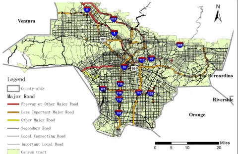
records were anonymized and de-identified prior to ana-lysis for protection of privacy. Term birth was defined as births occurring between 37 and 45 weeks of gestation. Multiple births (n= 35,213) were excluded as well as in-fants with recorded birth defects (n= 3353) or unknown birth defects status (n= 398). The study domain included 2043 Census tracts (Fig. 1), among which 1948 tracts remained for analysis after we removed those with too large an area (>50 km2, approximately the top 98.3 % per-centile by area;N= 37), too small sample size (less than 50 births;N= 29), islands (isolated Census tracts disconnected with any other tracts) (N= 12), or those with extreme values of term birth weight or covariates in the tracts (the outer fences [30] were used to filter the outlier tracts;N= 17). The 1.7 % very large tracts usually had a small popula-tion that were more heterogeneously distributed within the tracts than most of the other tracts, thus the statistics of environmental exposure and other parameters within the tract might not be representative of the whole tract. A very small sample size might introduce imprecision in model training, while the islands without neighbors would lead to difficulty in spatial modeling. Overall, we removed 95 (about 4.7 %) out of the 2043 tracts.
To study the association between air pollution and term birth weight, it is essential to obtain exposure
estimates at a fine spatiotemporal resolution since air pollution can be highly heterogeneous in time and space [31, 32] and the fetus is likely to be more sensitive to air pollution during specific time windows of exposure [33, 34]. We employed an advanced spatiotemporal models recently developed and validated in the same study re-gion [35] to estimate weekly NO2 and NOx
concentra-tions at the residence of each subject. Two major advantages of the models were the combination of long-term time-series data (high temporal but low spatial resolution) with dense sampling data from field cam-paigns (high spatial but low temporal resolution), and the incorporation of non-linear relationships between the predictor variables and the pollutant concentrations. The models showed good performance based on cross validation: for the weekly temporal trends, Pearson’s cor-relation was 0.84–0.91 for NO2and 0.81–0.90 for NOx
(-Additional file 1: Figures S1 and S2). We averaged weekly exposure estimates to compute exposures in each of the three trimesters of pregnancy and the entire pregnancy period (more details in Additional file 1: Section 1).
According to a priori knowledge [1, 4] and the de-scriptive statistics of this study, we included the follow-ing confoundfollow-ing factors in the models: maternal age, length of gestation, ethnicity, educational level, parity,
primary health care, and gender of the infant. In sensitivity analysis, we also tested the influence of pregnancy compli-cations (i.e. diabetes, hypertension and preeclampsia) and their influence was limited. All the confounders were dir-ectly retrieved from the birth certificates.
Laurent et al. [36] showed the beneficial effect of greenness (indicated by normalized difference vegetation index [NDVI]) on birth weight for a subset of the present study’s population; thus, we included NDVI in this analysis as well. NDVI within a 500 m buffer of each residence was extracted and averaged based on a set of mostly cloud-free Landsat scenes (resolution: 30 m) from the Global Land Survey 2005 (United States Geo-logical Survey) dataset covering Southern California.
Selection of the tract-level influential factors was based on a priori knowledge. We obtained information on these factors from the following sources:
(1)Community survey data from the TIGER 2006–2010 5-year estimation [37]. The community survey data included the socio-demographic factors (median household income, percentages of race/ethnicity [Hispanic, White, Black or Asian], female educational level) as well as the factors that may be related to air pollution exposure at the tract level but were not accounted for in the individual-level exposure estimates (percentages of the people driving cars, trucks or vans to work, walking or bicycling to work, commuting time shorter than 30 min, using utility gas for heating). The commuting patterns of the population may directly influence personal exposures to traffic-related pollutants [38]. For these variables, we aggregated the Census block data to Census tracts by weighting the area of blocks within a tract. (2)Land-use patterns. We obtained the 2008
parcel-level land-use data from the Southern California Association of Government (SCAG). The percentages of areas for the following land-uses were extracted for each tract: low/high density residential community, heavy industry (including manufacturing, petroleum refining and processing, major metal and chemical processing and mineral extraction), electrical power facilities, park and recreational space (including local, developed or undeveloped parks and recreations, wildlife preserves and sanctuaries, specimen gardens and arboreta and beach parks).
(3)Others: We obtained the 2005 TeleAtlas roadway network data from ArcGIS 10.1 (ESRI, Redlands, CA). The shortest distance to freeways/highways was calculated as the distance from the center point of each tract to the nearest freeways/highways. The same 30-m NDVI we used before for individual-level exposure was averaged over the entire area of each tract to characterize neighborhood greenspace.
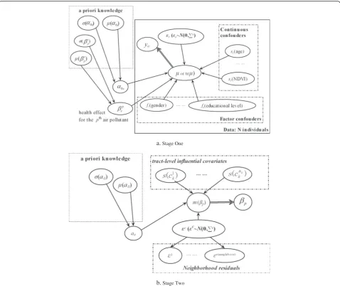
Based on the Bayesian framework, we developed a hierarchical two-stage model to: 1) quantify the associa-tions (effects) of individual air pollutants with term birth weight by adjusting for individual-level factors; and 2) investigate the influence of tract-level factors on the spatial variability of such effects.
Stage One: Within each Census tract, Bayesian addi-tive model was used to link term birth weight with air pollution exposure while adjusting for individual-level confounding factors:
yiceNðμic;σcÞ
μð Þyic ortrðμð Þyic Þ ¼a0cþxpcβpcþ
X
jsc xjc þ
X
kfcð Þ þxkc εc
μð Þ ¼yic E yicjAllμ ylc lð Þ≠i
8 > > < > > :
ð1Þ
wherecis the index of Census tract (c= 1,…,n),yicis the ith
individual term birth weight for the tract c, μ(yic) is
the expected value of the target variable (yic), tr(μ(yic)) is
the transformation (e.g. log, box-cox) of μ(yic), xcpis the
average of the pth air pollutant (NO2or NOx) during a
study period,a0c is the intercept,βcpis the regular health
effect (change in term birth weight per unit increase in ex-posure) of thepthair pollutant;xjcindicates thejth
continu-ous confounder such as NDVI and maternal age, while xkcindicates the factor variables such as race/ethnicity,
par-ity and educational level. sc() is a semi-parametric spline function and fc() is a factor function. yic, a0c and βcp
are assumed to be normally distributed: yic~N(μc,σc), a0c or βcp~N(0,σp). μ(yic) is the expected value of the ith
individual yic conditional on their neighborhood
[E(yic|All μ(ylc(l≠i)))] and modeled using spatial resid-uals, εc~N(0,Σc). Σc= [σijc] represents spatial
autocor-relation (σijc based on the distance between the ith and
jth
subject locations, modeled using the variogram).
We used Moran’s I [39] to determine the magnitude
of spatial autocorrelation and whether it is necessary
to incorporate it into the model [40]. In the end, we
did not include spatial autocorrelation in the stage one model since insignificant spatial autocorrelation was found for 91 % of the Census tracts.
The associations of air pollution with term birth weight were estimated based on a posterior distribution using full Bayesian inference via Markov Chain Monte Carlo (MCMC) simulation, which updated full condi-tionals of single or blocks of parameters [41]. Additional file 1: Section 2 presents the details for this.
Figure 2a shows the stage one model of our approach, in which the intercept (a0c) and effect coefficient of air pollutant (βpc) were assumed to be normally distributed and their hyper-parameters (mean:m; standard variance:
by the sample size (Additional file 1: Table S1). To avoid double counting, we excluded the meta-analysis papers and only included the individual studies that they cov-ered (plus other independent studies) without duplicates in the summary (Additional file 1: Figure S3). We also made sensitivity analyses using the pooled estimates re-ported by Stieb et al. [3] (−14.1 g per 10 ppb for NO2) as a prioriknowledge in the models.
Only a few published studies reported the association between NOx and term birth weight and mixed results
were observed [42]. Therefore, we assumed a uniform distribution of the NOx effect with a mean of 0 (no
ef-fect) with a standard deviation of 1 as non-informative prior knowledge [3, 43].
Stage Two: the effects (β) of air pollution on term birth weight were modeled against the tract-level covari-ates to examine their influence on spatial variability ofβ.
βpeNk m βp ;Vp
μ βp ¼h ηp ηp¼α0þ
Xmp
j¼1s cj þεp μ βp ¼E βpjNei βpj jð Þ≠c
8 > > > > > > < > > > > > > :
ð2Þ
where prepresents the pthair pollution exposure, μ(βp) represents the expected estimates forβp,h(ηp) is the link function for μ(βp) (h(ηp) =ηpfor normal distribution),cj
are the influential factors at the tract level, s(cj) is the
semi-parametric non-linear spline function for the factor
cj. The intercept, α0 represents the average estimate of
air pollution effect [α0~N(0,σp)]. εp is assumed to be spatially auto-correlative (εp|Σ~Np(0,Σp)) and is
mod-eled by spatially conditional auto-correlative regression (∑p= [σijp] represents spatial covariance) [44]. The
a. Stage One
b. Stage Two
variance ofβpmeasures the variability of the association between air pollution and term birth weight across
Cen-sus tracts. Moran’s I was used to determine whether
spatial autocorrelation of the effects of air pollution should be included in the stage two model.
The conditional expectation of the target variable (βp) incorporates spatial effects [41] and is determined by Census tract-level covariates and the weighted sum of the residuals of the effect coefficient from the means at neighborhoods [Nei(βpj(j≠c)) in Eq. (2)]. In this study,
spatial adjacency is based on the rook type that defines two tracts with at least one shared common boundary as neighbors [45]. The residual to incorporate spatial influ-ence from neighborhood is:
εp¼ρXj≠cwcj βpj−m βpj
ð3Þ
where ρ represents the effects of adjacent neighbors to
be estimated, wcj are spatial weights determining the
relative influence of neighborhood Census tract j on
Census tractc[44] (wcj= 1 if tractcis an adjacent
neigh-bor of tractj;wcj= 0 otherwise).
Point estimates (means) of the posterior effects of air pollutants and the impact of tract-level factors on the ef-fects were calculated based on the posterior distribution using full Bayesian inference in the stage two model, which is similar to Bayesian inference via Markov Chain Monte Carlo simulation in stage one. Additional file 1: Section 2 provides more details for the models. In the stage one and two models, we ran nine times of MCMC simulations and used the Gelman and Rubin approach to diagnose the convergence of the simulations to the stationary posterior distribution [45].
Figure 2b shows the stage two model of the Bayesian framework. The hyper-parameters (mean: μ; standard variance:σ) of the tract-level influential factors were de-termined according to a priori knowledge or as unin-formative priors. The outputs included the uncertainty of the posterior estimates of the effects, and the 95 % credible intervals (CI).
For evaluation of Bayesian hierarchical models, we used deviance information criterion (DIC) as a generalization of the Akaike information criterion and Bayesian informa-tion criterion. In Bayesian models, DIC has the advantage over other criteria mainly because it can be easily calcu-lated from the samples generated by a Markov Chain Monte Carlo simulation. Smaller values of DIC indicate a better fitting model.
Although some variables (e.g. ethnicity and NDVI) were simultaneously used in the stage one and two models, they represented individual-level characteristics in the stage one model, and neighborhood or context characteristics as aggregated features in the stage two model [46, 47]. We treated ethnicity as a categorical
variable in stage one, but as continuous variables (e.g. percentages of Hispanic, White, Black and Asian) in stage two. The NDVI was extracted as the average over a 500 m buffer of a specific residence in stage one but as the average over the entire Census tract in stage two.
Our models were constructed in R 3.2.1 (Bell Labora-tories, New Jersey, US) with the JAGS [48] and BayesX [49] packages. Details about the use of the packages are described in the last paragraph in Additional file 1: Sec-tion 2. We also include the main codes used for the two stage models as Additional files 2, 3, 4 and 5.
The study has been approved by the Institutional Re-view Board of the University of California, Irvine.
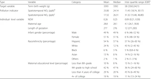
Results
Table 1 presents summary statistics (mean, median and inter-quartile range [IQR]) for the means of individual-level variables across 1948 Census tracts (statistics of Census tracts: mean area: 4.0 km2; variance of the areas: 26.9 km2). Mean term birth weight was 3393 g with an IQR of 58 g among all the tracts. Spatiotemporally-modeled NO2 and NOx exposures (IQR: 11.4 ppb for
NO2; 31.3 ppb for NOx) had high variability (defined as
standard variance divided by mean: 0.42 for NO2, 0.83
for NOx). Table 2 lists the statistics of the association
be-tween air pollution and term birth weight for each indi-vidual tract across all the tracts. Since a stronger association was found for exposure during the entire pregnancy than trimester-specific exposures (Table 2), we mainly reported the results for exposure during the entire pregnancy period. The DIC value was 454 for NO2 and 465 for NOx and the difference in DIC was
relatively small (Table 2).
From the existing literature, the summary of the prior effects of air pollution on term birth weight confirmed the normal distribution of the effect size (Additional file 1: Figure S3). Our sensitivity analysis showed limited influ-ence ofa prioriknowledge on posterior estimates (means NO2effect:−13.7 g per 10 ppb [our summary] vs.−13.9 g
per 10 ppb [Stieb’s pooled estimate]) despite the small to moderate differences ina prioriestimates using our sum-mary (as a priori knowledge, Additional file 1: Table S1 and Figure S3) vs. the pooled estimates [3].
Global Moran’s I tests showed spatially-clustering distri-bution of the associations between air pollutants and term birth weight. The Z-scores (6.4 for NO2; 6.1 for NOx) were
outside the range of−2.5 and 5.4 withp-value< 0.01, indi-cating moderate to strong spatial autocorrelation [50]. Therefore, we incorporated spatial effects in stage two.
birth weight (Additional file 1: Table S3) was −14.7 (95 % CI: −19.8, −9.7) g per 10 ppb for NO2, and−6.9
(95 % CI:−12.9,−0.9) g per 10 ppb for NOx.
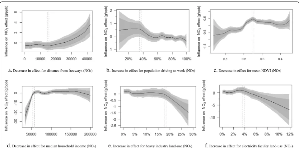
We found significant non-linear associations of exposure-related factors, socio-demographic factors, land-use patterns, and greenness with spatial variability of air pollution effects across Census tracts; the non-linear trends varied by these factors. The results of non-linear models (Additional file 1: Table S2) obscured significant nonlinear trends of such associations. The non-linear model captured the thresholds of the influential factors when their effects started to change markedly (Fig. 3 and Additional file 1: Figures S4 and S5). For illustration pur-poses, Additional file 1: Table S3 shows the changes in the average effects of air pollutants between the 1st and
the 4th quartiles of the tract-level factors, compared with the average posterior effects as the reference.
We found that the tracts further away from freeways/ highways generally had smaller reduction in term birth weights associated with exposure to NO2and NOx(less
weight reduction from the 1st to the 4th quartile of the distance: 3.7 g per 10 ppb for NO2; 4.9 g per 10 ppb for
NOx). The tracts with a higher percentage of the people
driving to work (approximately 36–60 %) were associ-ated with higher reduction in term birth weight for ex-posure to NO2 and NOx (more weight reduction from
the 1st to the 4th quartile of the percentage of the popu-lation driving to work: 1.6 g per 10 ppb for NO2; 14.7 g
per 10 ppb for NOx). Additionally, the tracts with more
people using gas for indoor heating had larger reduction Table 1Statistics for the means of the target and individual-level variable across Census tracts
Type Variable Category Mean Median Inter quartile range (IQR)a
Target variable Term birth weight (g) 3393 3392 58 (3363,3421)
Pollution indicator Spatiotemporal NO2(ppb)b 25.00 24.14 11.43 (18.74, 30.17)
Spatiotemporal NOx(ppb)c 17.32 26.31 31.32 (15.48, 46.80)
Individual- level variable NDVI 0.26 0.25 0.09 (0.21, 0.30)
Maternal age 28.8 28.1 4.1 (26.7, 30.8)
Length of gestation 277 276 12 (271,283)
Infant gender (percentage) Male 49 % 49 % 6 % (46–52 %)
Female 51 % 51 % 6 % (48–54 %)
Race/ethnicity (percentage) Hispanic 54 % 57 % 57 % (26–83 %)
White 24 % 12 % 43 % (2–45 %)
Black 6 % 3 % 5 % (0.8–6 %)
Asian 13 % 8 % 14 % (2–16 %)
Others 2 % 1 % 2 % (1–3 %)
Maternal educational level (percentage) Less than 8th grade 10 % 8 % 15 % (1–16 %)
9th grade to high school 42 % 47 % 36 % (24–60 %)
Less than 4 years of college 29 % 20 % 43 % (6–49 %)
4+ of college 19 % 19 % 11 % (13–24 %)
a
IQR for the mean (continuous variables) or percentage (categorical variables); b
Estimates of NO2by the spatiotemporal model;cEstimates of NOxby the spatiotemporal model
Table 2Statistics of the effectsaof NO2and NOxon term birth weight across all the tracts
Pollutants Period Mean (g/ppb) 95 % confidence intervals Mean of deviance
information criterion
NO2(ppb) 1st trimester −0.99 [−1.39,−0.59] 512
2st trimester −0.79 [−1.26,−0.32] 501
3st trimester −1.27 [−1.72,−0.82] 505
Entire Pregnancy −1.89 [−2.23,−1.55] 454
NOx(ppb) 1st trimester −0.54 [−0.80,−0.28] 514
2st trimester −0.52 [−0.78,−0.26] 512
3st trimester −0.61 [−0.90,−0.32] 512
Entire Pregnancy −0.87 [−1.09,−0.65] 465
a
in term birth weight from air pollution (more weight re-duction from the 1st to the 4th quartile of the percent-age of the population using gas for indoor heating: 1.8 g per 10 ppb for NO2; 17.4 g per 10 ppb for NOx).
For the tract-level socio-demographic factors, house-hold income, ethnicity and education level played im-portant roles in spatial variability of the health effects on term birth weight. Higher household income was associ-ated with smaller reduction in birth weight from air pol-lution exposure (less weight reduction from the 1st to the 4th quartile: 1 g per 10 ppb for NO2; 3.4 g per 10 ppb
for NOx). Race/ethnicity showed significant influence on
the effects of air pollution: a higher percentage of the Whites were associated with a lower risk of reduced birth weight from air pollution exposure (less weight reduction from the 1st to the 4th quartile: 0.3 g per 10 ppb for NO2). Further, a higher percentage (>10 %) of the women
with no or low education (below bachelor level) was asso-ciated with a higher risk of reduced birth weight from NO2exposure (more weight reduction by 5.1 g per 10 ppb
from the 1st to the 4th quartile).
For the land-use patterns, a higher percentage (>ap-proximately 18 %) of heavy-industry land-use (range: 0– 30 %) was linked to larger effects of NO2 and NOx on
reduced birth weight (more weight reduction by 13.0 g per 10 ppb of NO2and 3.9 g per 10 ppb of NOx, about
56–88 % of the tract-level posterior average effects, from the 1st to the 4th quartile of the percentage of heavy-industry land-use area]. A higher percentage (>5.8 % for NO2; >3.8 % for NOx) of electrical power facilities
land-use (range: 0–12 %) resulted in higher risks of NO2and
NOx (more weight reduction by 31.4–62.3 g per 10 ppb
from the 1st to the 4th quartile). Conversely, park and recreational land-use and NDVI (Fig. 3-f ) were respect-ively associated with smaller reduction in birth weight from NOx (less weight reduction by 6.7 g per 10 ppb
from the 1st to the 4th quartile) and NO2 (less weight
reduction by 4.8 g per 10 ppb from the 1st to the 4th quartile) exposure.
Spatial effects accounted for an important proportion (35–46 %) of the spatial variability of air pollution effect on term birth weight. Additional file 1: Figure S6 showed moderate-to-strong spatial clustering of the spatial dis-tribution of posterior effects of NO2(a) and NOx (b) on
term birth weight and the spatial clustering patterns were similar between the two pollutants. Additional file 1: Figure S7 presents the uncertainty of the results, i.e. the probability that air pollution effect is negative (adverse effect) in a given Census tract.
Discussion
Using the two-stage hierarchical Bayesian models, we quantified the effects of air pollution exposure on term birth weight and examined Census tract-level factors contributing to the spatial variability of such effects. Overall, the posterior estimates confirmed the negative association between air pollution exposure and term birth weight although the associations with NO2 were
more supported by the previous studies than that with NOx. The sensitivity analysis shows small difference
a. Decrease in effect for distance from freeways (NO2) b. Increase in effect for population driving to work (NO2) c. Decrease in effect for mean NDVI (NO2)
d. Decrease in effect for median household income (NOx) e. Increase in effect for heavy industry land-use (NOx) f. Increase in effect for electricity facility land-use (NOx)
between the prior effects of NO2and our posterior
esti-mates. This may reflect the consistency about the ad-verse effect of NO2 on term birth weight. The average
posterior output showed adverse effects of NO2 and
NOxon term birth weight: NO2and NOx may suppress
antioxidant defense system, cause lipid peroxidation and disturb fetus development, thus potentially leading to low birth weight [2].
To our knowledge, this is the first study employing the Bayesian non-linear approach to examine spatial vari-ability of the effects of air pollution on term birth weight across Census tracts and the factors contributing to such variability. Whereas the previous studies used the penal-ized smooth splines to adjust for the covariates [26, 27] or to simulate non-linear exposure-response associations [24, 25], this study used Bayesian hierarchical regression to quantify non-linear trends for the influence of the Census tract-level factors on the associations between ambient air pollutant concentrations and term birth weight, e.g. identifying the thresholds where the influ-ence had significant marked change, as shown in Fig. 3. Compared to the other non-linear methods, the Bayesian approach can minimize over-fitting by combining data with a priori knowledge; the latter is used as a penalty on the parameters (e.g. effects of NO2 on term birth
weight) to be learned to reflect the prior knowledge. Epi-demiological studies have frequently linked air pollution with adverse birth outcomes [3]. Based on the literature, we summarized the mean effect and the variance, and use them asa priori knowledge in the Bayesian models. The variances of a priori knowledge and the training sample determine the weights between both [43]: if the prior mean effect has a small variance, indicating rela-tively consistent findings from the previous studies, higher weight is assigned to the prior mean effect; con-versely, if the prior mean effect has a high variance, indi-cating heterogeneity in previous findings, lower weight is given to the prior mean effect and higher weight is given to the training sample. Thereby, the use of variances as the weights fora priori knowledge and data can effect-ively control the influence of over-smoothing by using the prior mean. Further, the incorporation of spatial ef-fects within the Bayesian model enabled the identifica-tion of spatial patterns of the adverse effects of NO2and
NOxon term birth weight.
The emissions of air pollutants not accounted for by NO2 and NOx exposures may influence the spatial
vari-ability of the effects of the two pollutants on term birth weight. Being away from freeway/highway might lead to lower local traffic-related air pollutant exposure and lower noise exposure at residential locations, thus lowering the effect of NO2 and NOx at the Census tract level. We
found lower risk of air pollution for reduction in term birth weight in Census tracts with a higher percentage of
people biking or walking to work, or with a higher per-centage of people who commute less than 30 min to work. For the working population taking vehicles, average ex-posure to traffic-related pollutants may be higher due to their exposure in commutes [38]. Further, more work-related commutes may increase the concentrations of traffic-related air pollution in local communities that were not captured by the spatiotemporal models for NO2and
NOx. Additionally, long commuting time is likely
associ-ated with a higher stress level (e.g. driving activity itself and shorter time with family) that might lead to the ob-served higher risk associated with air pollution [8, 51].
Besides ambient pollution, we observed that house heat-ing was significantly associated with increase of the tract-level adverse effects. This may indicate an effect of increased exposure to indoor air pollution [52]. Although house heating is uncommon in Los Angeles, the availabil-ity of gas heaters may indicate a 50 % probabilavailabil-ity of use of gas stove at least for cooking according to the US Residen-tial Energy Consumption Survey [53, 54]. Gas stove use may increase indoor concentrations of NO2, particulate
matter and other pollutants [52, 55, 56], which may add to the observed risk of NO2and NOx.
This study suggests important influence of socio-demographic factors. Higher household income reflects higher SES and likely lower vulnerability to the effects of air pollution, consistent with the previous studies [9, 57]. Results also showed a non-linear trend: beyond the thresh-old of about $40,000–60,000, the influence of income on the effects of air pollution became much weaker [58].
Further, Census tracts with a higher percentage of Whites had a lower risk of reduced birth weight. Previ-ous studies [6, 57, 59] consistently showed weaker ad-verse effects of air pollution in White mothers than in African American mothers. Besides genetic differences, SES in different race groups may also contribute to the observed differences in health effects. In our study popu-lation, tract-level median household income was nega-tively associated with the percentage of African Americans and positively correlated with the percentage of Whites (Pearson’s correlation:−0.19 vs. 0.54).
Higher maternal education may indicate higher SES, more knowledge on potential adverse effects of environ-mental agents, and healthier life style, which may reduce the adverse effects of air pollution on pregnancy outcomes. Our results agree with a number of previous studies that linked lower maternal educational level with adverse preg-nancy outcomes including term low birth weight [6].
spatiotemporal models. Heavy industry might also be as-sociated with other environmental insults such as noise. Further, we found a non-linear trend, with a threshold (approximately 18 % of area) for heavy industrial land-use, above which the influence was noticeably exacerbated for the effects of NO2and NOx. Further, the land-use of
elec-trical power facilities had significant influence on the effects. Electrical power facilities included electric power installa-tion, welding, induction heaters and electrified transport sys-tems that were important sources of extremely low frequency fields [60]. We found non-linearly increased ad-verse effects of air pollution on term birth weight beyond the threshold of 3.8–5.8 % of area for electrical power facil-ities. Several studies [61–63] showed adverse influence of the extremely low frequency fields on pregnant women. A possible mechanism for this is that the extremely low fre-quency fields might disturb the balance between plasma and vascular cell Ca2+, subsequently resulting in disruption of placental vascular function change and suboptimal growth of the fetus, thus potentially impairing fetal growth. How-ever, more investigation is required to evaluate whether the electrical power facility land-use as a neighborhood factor might aggravate the adverse effects of air pollution.
Contrarily, the exposure to the park and recreational land-use and greenness was associated with a smaller re-duction in term birth weight from NO2and NOx
expos-ure. A higher value of the two variables might be associated with more active social and physical activities in the neighborhoods [64], reduced local temperature and exposure level to air pollution and noise, and less stress [65]. Our findings on the beneficial effects of greenness are consistent with the previous studies [36, 64, 66].
Traditional regression analysis, without considering spatial effects, may generate the estimates with spatially auto-correlative residuals [67]. In this study, NO2 and
NOx had similar patterns of spatial clustering. Strong
spatial patterns might indicate significant influence of the regional factors such as regional patterns (potentially cor-related with pregnancy outcomes) in diet and lifestyle, and surrounding terrain or physical setting (not included in the model) on the health effects of air pollution.
Our finding of spatially varying effects of air pollution is consistent with the recent finding of Coker et al. [13] for the same study region (Los Angeles). Our study advanced the previous studies [12–14] by using Bayesian hierarch-ical models to assess which factors contributed to the varying spatial effects of air pollution. We identified the tract-level factors that attenuate or exacerbate the associ-ation between air pollutants and term birth weight.
This study has several limitations. First,a priorieffect of air pollution on term birth weight was derived from a limited number of studies that either used air pollution measures of relatively coarse spatial resolution or used simplistic regression models. To minimize the potential
inconsistency and bias in the estimation of air pollution effects, we incorporated the variance of the prior evi-dence as an uncertainty indicator and used it as weights between data learning and a priori knowledge. Second, although advanced spatiotemporal models were used to estimate air pollutant concentrations, there was still un-certainty in estimating the personal exposure of preg-nant women. We did not consider exposures at workplace and in vehicles. In addition, we relied on the address at delivery for exposure assessment and did not consider the change of address during pregnancy due to a lack of data. This might introduce exposure misclassifi-cation for a limited number of mothers. Third, we did not account for the influence of multiple pollutants. However, it is difficult to put the pollutants together in one model since this may introduce co-linearity (we found strong correlation [Pearson’s r = 0.81] between NO2and NOx). Fourth, although our non-linear models
detected the thresholds of the land-use from which the in-fluences on the effects of air pollutants had pronounced var-iations, such thresholds may vary across cities or regions. For example, the heavy-industry land-use may be affected by the type of industry, spatial distribution of population and emission sources, and thus such threshold may vary by city. In addition, the greenness indicator of NDVI did not specify types of vegetation, which may differ by region and have different influence on the effects of air pollutants. However, the spatial effect included in our models might partially account for such confounding effects. Fifth, our ap-proach quantified the associations between the influential factors and the effects of air pollutants, but such associations were not necessarily causal. For example, the distance from highway may just represent suburban tracts, which are very different from the urban tracts.
Conclusions
Additional files
Additional file 1:Section 1.Spatiotemporal models for exposure estimation of NO2and NOx.Section 2.Two-stage models.Table S1.
Effects of NO2and NOxon birth weight from the previous studies. Table S2.Contribution of each tract-level factor in linear models to the NO2and NOxeffects.Table S3.Change in effects of NO2and NOx
-between the 1st and 4th quartiles of each tract-level factor in non-linear models.Figure S1.NO2and NOxtime series predicted by the spatiotemporal
model.Figure S2.NO2(a) and NOx(b) long-term averages of the predicted
time series vs. the measurements for all the 25 stations.Figure S3.A priori
statistics of the effects of NO2on birth weight summarized from the previous
studies (Table S1).Figure S4.Non-linear effects of NO2on birth weight
(smooth term) from Stage Two.Figure S5.Non-linear effects of NOxon birth
weight (smooth term) from Stage Two.Figure S6.Posterior estimates of the effects of NO2and NOx.Figure S7.Probability map of the Census tract NO2
and NOxeffects for term birth weight [P(β< 0)]. (PDF 1852 kb)
Additional file 2:Stage one no2: Code file for the stage one model for NO2. (R 6 kb)
Additional file 3:Stage one nox: Code file for the stage one model for NOx. (R 5 kb)
Additional file 4:Stage two no2: Code file for the stage two model for NO2. (R 5 kb)
Additional file 5:Stage two nox: Code file for the stage two model for NOx. (R 5 kb)
Abbreviations
CI:Credible intervals; DIC: Deviance information criterion; IQR: inter-quartile range; MCMC: Markov Chain Monte Carlo; NDVI: Normalized difference vegetation index; NO2: Nitrogen dioxide; NOx: Nitrogen oxides; PM: Particular
matter; PM2.5: Particular matter with diameter <2.5μm; SCAG: Southern
California Association of Government; SES: Socioeconomic status.
Competing interests
The authors declare that they have no competing interests.
Authors’contributions
LL contributed to the study conception, constructed the Bayesian hierarchical models, performed all statistical analyses, and drafted the manuscript. OL processed the data of the birth certificate records and contributed to acquirement ofa prioriknowledge and the manuscript’s revision. JW contributed to the introduction of this study’s background, adjustment of the models and the manuscript’s revision. All authors reviewed and approved the final manuscript.
Acknowledgments
The study was supported by the Health Effect Institute (HEI 4787-RFA09-4110-3 WU) and the Natural Science Foundation of China (41471376, 41171344). The authors gratefully acknowledge the data support from US Census Bureau and constructive comments from the reviewers. They also acknowledge Jason Li for his help in editing the manuscript.
Author details
1
Program in Public Health, College of Health Sciences, University of California, Anteater Instruction & Research Bldg (AIRB) # 2034, 653 East Peltason Drive, Irvine, CA 92697-3957, USA.2State Key Lab of Resources and Environmental Information Systems, Institute of Geographical Sciences and Natural Resources Research, Chinese Academy of Sciences, A11 Datun Road, Anwai, Chaoyang, Beijing 100101, China.
Received: 16 June 2015 Accepted: 1 February 2016
References
1. Proietti E, Roosli M, Frey U, Latzin P. Air pollution during pregnancy and neonatal outcome: a review. J Aerosol Med Pulm Drug Deliv. 2013;26(1):9–23. 2. Shah PS, Balkhair T. Air pollution and birth outcomes: a systematic review.
Environ Int. 2011;37(2):498–516.
3. Stieb DM, Chen L, Eshoul M, Judek S. Ambient air pollution, birth weight and preterm birth: a systematic review and meta-analysis. Environ Res. 2012; 117:100–11.
4. Bonzini M, Carugno M, Grillo P, Mensi C, Bertazzi A, Pesatori C. Impact of ambient air pollution on birth outcomes: systematic review of the current evidences. Med Lav. 2010;101(5):341–63.
5. Dominici F, Sheppard L, Clyde M. Health effects of air pollution: a statistical review. Int Stat Rev. 2003;71(2):243–76.
6. Sram RJ, Binkova B, Dejmek J, Bobak M. Ambient air pollution and pregnancy outcomes: a review of the literature. Environ Health Perspect. 2005;113(4):375–82.
7. Strickland MJ, Klein M, Darrow LA, Flanders WD, Correa A, Marcus M, et al. The issue of confounding in epidemiological studies of ambient air pollution and pregnancy outcomes. J Epidemiol Community Health. 2009;63(6):500–4. 8. Gray SC, Edwards SE, Schultz BD, Miranda ML. Assessing the impact of race,
social factors and air pollution on birth outcomes: a population-based study. Environ Health. 2014;13(1):4.
9. Zeka A, Melly SJ, Schwartz J. The effects of socioeconomic status and indices of physical environment on reduced birth weight and preterm births in Eastern Massachusetts. Environ Health. 2008;7:60.
10. Dadvand P, Parker J, Bell ML, Bonzini M, Brauer M, Darrow LA, et al. Maternal exposure to particulate air pollution and term birth weight: a multi-country evaluation of effect and heterogeneity. Environ Health Perspect. 2013;121(3): 267–373.
11. Parker JD, Rich DQ, Glinianaia SV, Leem JH, Wartenberg D, Bell ML, et al. The international collaboration on air pollution and pregnancy outcomes: initial results. Environ Health Perspect. 2011;119(7):1023–8.
12. Williams BL, Pennock-Roman M, Suen HK, Magsumbol MS, Ozdenerol E. Assessing the impact of the local environment on birth outcomes: a case for HLM. J Expo Sci Environ Epidemiol. 2007;17(5):445–57.
13. Coker E, Ghosh J, Jerrett M, Gomez-Rubio V, Beckerman B, Cockburn M, et al. Modeling spatial effects of PM on term low birth weight in Los Angeles County. Environ Res. 2015;142:354–64.
14. Hao Y, Strosnider H, Balluz L, Qualters JR. Geographic variation in the association between ambient fine particulate matter (PM2.5) and term low
birth weight in the United States. Environ Health Perspect. 2015. doi:10. 1289/ehp.1408798.
15. Levy I, Mihele C, Lu G, Narayan J, Brook JR. Evaluating multipollutant exposure and urban air quality: pollutant interrelationships, neighborhood variability, and nitrogen dioxide as a proxy pollutant. Environ Health Perspect. 2014;122(1):65–72.
16. US Census Bureau. Census Tracts and Block Numbering Areas. 2000. https:// www.census.gov/history/www/programs/geography/tracts_and_block_ numbering_areas.html. Accessed 12 Dec 2015.
17. English PB, Kharrazi M, Davies S, Scalf R, Waller L, Neutra R. Changes in the spatial pattern of low birth weight in a southern California county: the role of individual and neighborhood level factors. Soc Sci Med. 2003;56(10):2073–88. 18. Anselin L. Discrete space autoregressive models. In: Goodchild M, Parks B,
Steyaert L, editors. Environmental modeling with GIS. New York: Oxford University Press; 1993. p. 454–69.
19. Li L, Wang J, Wu J. A spatial model to predict the incidence of neural tube defects. BMC Public Health. 2012;12:951.
20. Kallenberg O. Foundations of modern probability. New York: Springer; 1997. 21. Gelman A, Carlin BJ, Stern SH, Rubin BD. Bayesian data analysis. Florida:
Chapman & Hall/CRC; 2004.
22. Currie J, Neidell M. Air pollution and infant health: what can we learn from California’s recent experience? Q J Econ. 2005;120(3):1003–30.
23. Zhou Y, Hammitt J, Fu JS, Gao Y, Liu Y, Levy JI. Major factors influencing the health impacts from controlling air pollutants with nonlinear chemistry: an application to China. Risk Anal. 2014;34(4):683–97.
24. Ha EH, Hong YC, Lee BE, Woo BH, Schwartz J, Christiani DC. Is air pollution a risk factor for low birth weight in Seoul? Epidemiology. 2001;12(6):643–8. 25. Savitz DA, Bobb JF, Carr JL, Clougherty JE, Dominici F, Elston B, et al.
Ambient fine particulate matter, nitrogen dioxide, and term birth weight in New York, New York. Am J Epidemiol. 2014;179(4):457–66.
26. Gouveia N, Bremner SA, Novaes H. Association between ambient air pollution and birth weight in Sao Paulo, Brazil. J Epidemiol Community Health. 2004;58(1):11–7.
28. Hastie TJ. Generalized additive models. New York: Chapman and Hall; 1990. 29. Laurent O, Hu J, Li L, Cockburn M, Escobedo L, Kleeman MJ, et al. Sources
and contents of air pollution affecting term low birth weight in Los Angeles County, California, 2001–2008. Environ Res. 2014;134:488–95.
30. Iglewicz B, Hoaglin CD. How to detect and handle outliers. In: Mykytka FE, editor. The ASQ basic references in quality control: Statistical techniques. Milwaukee: American Society for Quality; 1993. p. 1–87.
31. Mercer DL, Szpiro AA, Sheppard L, Lindstrom J, Adar DS, Allen WR, et al. Comparing universal kriging and land-use regression for predicting concentrations of gaseous oxides of nitrogen (NOx) for Multi-Ethnic Study of Attherosclerosis and Air Pollution (MESA AIR). Atmos Environ. 2011;45:4412–20. 32. Zhu Y, Hinds W, Kim S, Shen S, Sioutasc S. Study of ultrafine particles near a major highway with heavy-duty diesel traffic. Atmos Environ. 2002;36(27): 4323–35.
33. Geer LA, Weedon J, Bell ML. Ambient air pollution and term birth weight in Texas from 1998 to 2004. J Air Waste Manage Assoc. 2012;62(11):1285–95. 34. Rose N, Cowie C, Gillett R, Marks BG. Validation of a spatiotemporal land use
regression model incorporating fixed site monitors. Environ Sci Technol. 2011;45(1):294–9.
35. Li L, Wu J, Ghosh JK, Ritz B. Estimating spatiotemporal variability of ambient air pollutant concentrations with a hierarchical model. Atmos Environ. 2013; 71:54–63.
36. Laurent O, Wu J, Li L, Milesi C. Green spaces and pregnancy outcomes in Southern California. Health Place. 2013;24:190–5.
37. US Census Bureau. TIGER/Line® with Selected Demographic and Economic Data. 2012.http://www.census.gov/geo/maps-data/data/tiger-data.html. Accessed 12 Dec 2015.
38. Wu J, Tjoa T, Li L, Jaimes G, Delfino RJ. Modeling personal particle-bound polycyclic aromatic hydrocarbon (pb-pah) exposure in human subjects in Southern California. Environ Health. 2012;11:47.
39. Getis A, Ord KJ. The analysis of spatial association by use of distance statistics. Geogr Anal. 2010;24:189–206.
40. Dormann CF. Response to comment on“Methods to account for spatial autocorrelation in the analysis of species distributional data: a review”. Ecography. 2009;32(3):379–81.
41. Fahrmeir L, Lang S. Bayesian inference for generalized additive mixed models based on Markov random field priors. J Roy Stat Soc C-App. 2001; 50:201–20.
42. Pedersen M, Giorgis-Allemand L, Bernard C, Aguilera I, Andersen AM, Ballester F, et al. Ambient air pollution and low birthweight: a European cohort study (ESCAPE). Lancet Respir Med. 2013;1(9):695–704. 43. Carlin PB, Louis TA. Bayesian methods for data analysis (third edition).
Florida: Taylor & Francis Group, LLC; 2009.
44. Cressie N. Statistics for spatial data, revised edition. NY: Wiley; 1993. 45. Belitz C, Brezger A, Klein N, Kneib T, Lang S, Umlauf N. BayesX: Methodology
Manual; 2015. http://www.statistik.lmu.de/~bayesx/manual/methodology_ manual.pdf. Accessed 12 Dec 2015.
46. Macintyre MS, Ellaway A, Cummins S. Place effects on health: how can we conceptualise, operationalise and measure them? Soc Sci Med. 2002;55:125–39. 47. Pickett KE, Pearl M. Multilevel analyses of neighbourhood socioeconomic
context and health outcomes: a critical review. J Epidemiol Community Health. 2001;55(2):111–22.
48. Plummer M. JAGS: a program for analysis of Bayesian graphical models using Gibbs sampling. In: Hornik K., Leisch F. and Zeileis A. (Eds.) Proceedings of the 3rd International Workshop on Distributed Statistical Computing. 2003. Vienna, Austria. Published as http://www.ci.tuwien.ac.at/ Conferences/DSC-2003/.
49. Brezger A, Lang S. Generalized structured additive regression based on Bayesian P-Splines. Comput Stat Data Anal. 2006;50:967–91.
50. Ebdon D. Statistics in geography: A practical approach. Oxford: Blackwell; 1985. 51. Sable MR, Wilkinson DS. Impact of perceived stress, major life events and
pregnancy attitudes on low birth weight. Fam Plann Perspect. 2000;32(6): 288–94.
52. Logue JM, Klepeis NE, Lobscheid AB, Singer BC. Pollutant exposures from natural gas cooking burners: a simulation-based assessment for Southern California. Environ Health Perspect. 2014;122(1):43–50.
53. KEMA-XENERGY, Itron, RoperASWCEC. California Statewide Residential Appliance Saturation Study. Final Report. 400-04-009. California Energy Commission. 2014. http://www.energy.ca.gov/reports/400-04-009/2004-08-17_400-04-009VOL2B.PDF. Accessed 12 Dec 2015.
54. US Energy Information Administration. Residential Energy Consumption Survey. 2009. https://www.eia.gov/consumption/residential/data/2009/. Accessed 12 Dec 2015.
55. Nicole W. Cooking up indoor air pollution: emissions from natural gas stoves. Environ Health Perspect. 2014;122(1):A27.
56. Vrijheid M, Martinez D, Aguilera I, Bustamante M, Ballester F, Estarlich M, et al. Indoor air pollution from gas cooking and infant neurodevelopment. Epidemiology. 2012;23(1):23–32.
57. Padula AM, Mortimer K, Hubbard A, Lurmann F, Jerrett M, Tager IB. Exposure to traffic-related air pollution during pregnancy and term low birth weight: estimation of causal associations in a semiparametric model. Am J Epidemiol. 2012;176(9):815–24.
58. Phelps CE. Health economics. Addison Wesley: Boston; 2003.
59. Maisonet M, Bush TJ, Correa A, Jaakkola JJK. Relation between ambient air pollution and low birth weight in the northeastern United States. Environ Health Perspect. 2001;109:351–6.
60. SCENIHR. Health Effects of Exposure to EMF. Brussels of Belgium; European Commission. 2009.
61. Adamova Z, Ozkan S, Khalil RA. Vascular and cellular calcium in normal and hypertensive pregnancy. Curr Clin Pharmacol. 2009;4(3):172–90.
62. de Vocht F, Hannam K, Baker P, Agius R. Maternal residential proximity to sources of extremely low frequency electromagnetic fields and adverse birth outcomes in a UK cohort. Bioelectromagnetics. 2014;35(3):201–9. 63. de Vocht F, Lee B. Residential proximity to electromagnetic field sources
and birth weight: Minimizing residual confounding using multiple imputation and propensity score matching. Environ Int. 2014;69:51–7. 64. Dadvand P, de Nazelle A, Figueras F, Basagana X, Su J, Amoly E, et al. Green
space, health inequality and pregnancy. Environ Int. 2012;40:110–5. 65. Paoletti E, Bardelli T, Giovannini G, Pecchioli L. Air quality impact of an
urban park over time. Procedia Environ Sci. 2011;4:10–6.
66. Donovan GH, Michael YL, Butry DT, Sullivan AD, Chase JM. Urban trees and the risk of poor birth outcomes. Health Place. 2011;17(1):390–3.
67. Parker JD, Woodruff TJ. Influences of study design and location on the relationship between particulate matter air pollution and birth weight. Paediatr Perinat Epidemiol. 2008;22(3):214–27.
• We accept pre-submission inquiries
• Our selector tool helps you to find the most relevant journal
• We provide round the clock customer support
• Convenient online submission
• Thorough peer review
• Inclusion in PubMed and all major indexing services
• Maximum visibility for your research
Submit your manuscript at www.biomedcentral.com/submit