R E S E A R C H A R T I C L E
Open Access
Network meta-analysis on the log-hazard scale,
combining count and hazard ratio statistics
accounting for multi-arm trials: A tutorial
Beth S Woods
1*, Neil Hawkins
1,2, David A Scott
1Abstract
Background:Data on survival endpoints are usually summarised using either hazard ratio, cumulative number of events, or median survival statistics. Network meta-analysis, an extension of traditional pairwise meta-analysis, is typically based on a single statistic. In this case, studies which do not report the chosen statistic are excluded from the analysis which may introduce bias.
Methods:In this paper we present a tutorial illustrating how network meta-analyses of survival endpoints can combine count and hazard ratio statistics in a single analysis on the hazard ratio scale. We also describe methods for accounting for the correlations in relative treatment effects (such as hazard ratios) that arise in trials with more than two arms. Combination of count and hazard ratio data in a single analysis is achieved by estimating the cumulative hazard for each trial arm reporting count data. Correlation in relative treatment effects in multi-arm trials is preserved by converting the relative treatment effect estimates (the hazard ratios) to arm-specific outcomes (hazards).
Results:A worked example of an analysis of mortality data in chronic obstructive pulmonary disease (COPD) is used to illustrate the methods. The data set and WinBUGS code for fixed and random effects models are provided. Conclusions:By incorporating all data presentations in a single analysis, we avoid the potential selection bias associated with conducting an analysis for a single statistic and the potential difficulties of interpretation, misleading results and loss of available treatment comparisons associated with conducting separate analyses for different summary statistics.
Background
Network meta-analyses enable us to combine trials that compare different sets of treatments, and form a net-work of evidence, within a single analysis [1] and to use all available direct and indirect evidence to inform a given comparison between treatments. Network meta-analysis is based on the assumption that, on a suitable scale, we can add and subtract within-trial estimates of relative treatment effects i.e. the difference in effect between treatments A & B (dAB) is equal to the
differ-ence in effects between treatments A & C and B & C (dAB=dAC- dBC) [1-3].
In this paper we show how network meta-analyses of survival endpoints can be conducted on the hazard ratio
scale when some or all trials report cumulative count data. We also describe how trials with more than two arms reporting relative treatment effects (such as hazard ratios) should be included.
A survival endpoint is one where, over time, an increasing number of patients experience an event. Although death is the ultimate survival endpoint, many other endpoints may also be considered as survival end-points. For example, in the study of epilepsy, seizure freedom may be regarded as a survival endpoint as over time the number of patients experiencing one or more seizures can only increase and the probability of being seizure free decreases. In contrast, the number of patients with a greater than 50% reduction in seizure frequency relative to baseline is not a survival endpoint as the number of patients achieving this response can increase or decrease over time.
* Correspondence: [email protected]
1
Oxford Outcomes Ltd., Oxford, UK
Data on survival endpoints may be expressed either in the form of hazard ratio statistics derived from para-metric or non-parapara-metric methods of survival analysis [4,5] or as cumulative count statistics (the total number of subjects who have experienced an event at a specific time point). Unlike cumulative count statistics, hazard ratio statistics from survival analysis account for censor-ing, incorporate time to event information, and may be adjusted for co-variables. Where both hazard ratio and cumulative count statistics are available for a given study, use of the hazard ratio data may therefore be considered preferable.
The methods described in this paper allow hazard ratio and cumulative count survival statistics to be com-bined within a single network meta-analysis on the log-hazard scale; this might be termed a multi-statistic evi-dence synthesis. Treatment effects can then be esti-mated based on an inclusive set of data, and separate analyses for hazard ratio and count statistics are avoided [6-9].
Network meta-analyses should account for the corre-lations in relative treatment effect estimates that arise from trials with more than two treatment arms (multi-arm trials) [10]. These correlations are accounted for‘by default’ when count statistics for individual trial arms are included in a network meta-analysis [10]. When hazard ratio statistics are used, we show how these cor-relations can be accounted for by deriving estimates of the mean log hazards (and their variances) for individual trial arms.
Methods
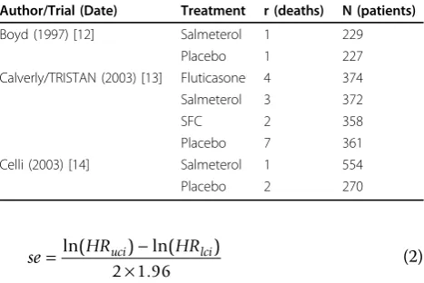
We use an example data set describing mortality in randomised controlled trials of treatments for chronic obstructive pulmonary disease (COPD). The data set consists of a subset of trials from Baker et al [11]. We chose five trials providing mortality data for the fol-lowing comparators: salmeterol, fluticasone, salmeterol fluticasone combination (SFC) or placebo. Three of the trials report count data [12-14], one reports hazard ratio data from a two arm trial [15] and one reports hazard ratio data from a multi (four)-arm trial [16]. Hazard ratio data were obtained from the trial publications and an existing meta-analysis of hazard ratio data [17].
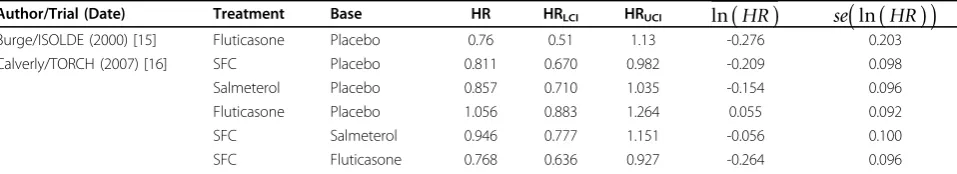
The count statistics used are presented as Table 1 and the hazard ratio statistics as Table 2. The derived
esti-mates of the mean log hazard ratio and it’s standard
error, required for the analysis, are also presented in Table 2, these were estimated using formulae (1) and (2):
ln(HR)= ln(HRuci)+ln(HRlci)
2 (1)
se= HRuci − HRlci ×
ln( ) ln( )
.
2 1 96 (2)
The results of this example analysis are purely illustra-tive of the methodology and do not provide any indica-tion of the comparative effectiveness of treatments for decision-making purposes, as the data set omits relevant direct and indirect data.
Using the example data set we show how to:
(a) Perform a meta-analysis of count statistics on the log hazard ratio scale;
(b) Reflect correlation in relative treatment effect estimates from multi-arm trials;
(c) Combine count and hazard ratio statistics in a single analysis on the log-hazard ratio scale; and (d) Include a random effect in to the analysis, whilst preserving the correlation in relative treatment effects for multi-arm trials.
We also discuss how other possible presentations of survival data, not available from our motivating exam-ple, could be incorporated into an analysis on the log-hazard ratio scale.
All analyses described were conducted using Win-BUGS [18]. The WinWin-BUGS code for the fixed and ran-dom effects analyses are presented as an Appendix.
(a) Meta-analysing count statistics on the log hazard ratio scale
The count data are incorporated in the network meta-analysis model using a binomial likelihood:
rs k, ~Bin F( s k, ,ns k, ) (3)
where rs,k is the cumulative count of subjects who
have experienced an event in armkof study s;ns,kis the
total number of subjects in arm kof studys; andFs,kis
the cumulative probability of a subject having experi-enced an event (or‘failure’).
Table 1 Count Statistics
Author/Trial (Date) Treatment r (deaths) N (patients)
Boyd (1997) [12] Salmeterol 1 229
Placebo 1 227
Calverly/TRISTAN (2003) [13] Fluticasone 4 374
Salmeterol 3 372
SFC 2 358
Placebo 7 361
Celli (2003) [14] Salmeterol 1 554
A log cumulative hazard for each trial arm ln(Hs,k) is
then derived fromFs,k.
ln(Hs k, )=ln
(
−ln(
1−Fs k,)
)
(4)The log cumulative hazard estimates are then included in a treatment effect model with a linear regression structure. The log cumulative hazard is estimated as the sum of a study specific ‘baseline’term asand a
treat-ment effect coefficientbk:
ln(Hs k, )=s+k−b (5)
whereb1 = 0 for the reference treatment (placebo in our example) andbbrepresents the treatment effect for
the baseline treatment in study s. The fixed study level
‘baseline’ term is a nuisance parameter, included to
ensure that the treatment effect estimates are informed by within trial differences between treatment arms and not by differences in baseline event rates across trials.
Under an assumption of proportional hazards, the bk
coefficient is equal to both the log cumulative hazard ratio and the log hazard ratio:
ln exp( ) ,
, ln
exp( ) ,
,
k hs b
hs b
k hs b t
hs b t ⋅
⎛ ⎝
⎜⎜ ⎞⎠⎟⎟ =
⋅ ∫
∫ ⎛
⎝ ⎜ ⎜ ⎜ ⎜ ⎜ 0
0
⎞⎞
⎠ ⎟ ⎟ ⎟ ⎟ ⎟
=k(6)
wherehs,brepresents the hazard for the baseline
treat-ment in studys. This identity allows us to combine the count statistics analysed on the log cumulative hazard scale with the hazard ratio data analysed on the log hazard scale. It also demonstrates that analysis of count statistics on the log hazard scale does not require a stronger assumption than proportional hazards.
(b) Reflecting correlations in relative treatment effects from multi-arm trials
Estimates of relative treatment effects from trials with more than two treatment arms will be correlated [10]. In our example the TORCH trial [16] is the only
multi-arm trial reporting hazard ratio data. Estimated treatment effects from TORCH will be correlated, for example, the hazard ratio comparing SFC to placebo and the hazard ratio comparing salmeterol to placebo will be correlated due to their joint dependence on the time to event data in the placebo arm.
If a network meta-analysis is based on estimates of treatment effect in individual trial arms rather than estimates of relative treatment effect between arms (“contrast” statistics), this correlation will automatically be captured in the analysis [10]. This is the case when a network meta-analysis is based on count statistics. However, if the network meta-analysis is conducted based on estimates of relative treatment effect, this correlation between arms will not automatically be captured [10].
For multi-arm trials reporting hazard ratio statistics, this problem can be addressed by converting the log hazard ratios (contrast statistics) to log hazards (arm-specific statistics). Log hazards for individual trial arms are derived by nominally setting the log hazard for the baseline treatment bfor the trial to zero. The mean log hazards for the other treatments are then equal to the log hazard ratios compared to baseline treatment.
The variance for a log hazard ratio is the sum of the variances for the individual log hazards. Standard errors of the log hazards for each trial arm can therefore be estimated by solving simultaneous equations based on the standard errors for the set of log-hazard ratios. For example:
seb =
(
(sek b1, +sek b2, −sek k1, 2) /)
2 2 2
2 (7)
Where se2i,j is the variance of the log hazard ratio
comparing armi to armjandsei is the standard error
of the log hazard for armi.
The standard errors of the log hazards for the other treatment arms are then estimated as:
sek = sek b2, −seb2 (8)
Mean log hazards and associated standard errors for each treatment in TORCH [16] are reported in Table 3. Table 2 Hazard ratio and log hazard ratio statistics
Author/Trial (Date) Treatment Base HR HRLCI HRUCI ln
(
HR)
se(
ln(
HR)
)
Burge/ISOLDE (2000) [15] Fluticasone Placebo 0.76 0.51 1.13 -0.276 0.203
Calverly/TORCH (2007) [16] SFC Placebo 0.811 0.670 0.982 -0.209 0.098
Salmeterol Placebo 0.857 0.710 1.035 -0.154 0.096
Fluticasone Placebo 1.056 0.883 1.264 0.055 0.092
SFC Salmeterol 0.946 0.777 1.151 -0.056 0.100
These are derived from the hazard ratio data presented in Table 2.
In order to estimate standard errors of the log hazards for each treatment, we required estimates of the uncer-tainty associated with four treatment contrasts. In some cases this data may not be available and thus the meth-ods presented in equations 7 and 8 may not be feasible. For example, hazard ratios and associated measures of uncertainty may only be available for each active treat-ment relative to a single common comparator (e.g. pla-cebo) as is commonly reported in the published literature.
In this situation, we can approximate the standard error for the comparison between active treatments by assuming the standard error is proportional to 1n . For example
sek k sek b sek b nk nk nk nk nb
1 2 1 2 1 2 1 2
2 2 1 1 1 1 2
, =
(
(
(
, + ,)
⋅(
+)
)
(
+ +)
)
(9)(c) Combining count and hazard ratio statistics in a network meta-analysis
The log hazard ratio statistics from two arm trials
comparing treatments k to b are incorporated in the
network meta-analysis model using a normal likelihood:
x hs k
hs b se s k b, , ~ ln , s k b, ,
, ,
N ⎛
⎝ ⎜⎜ ⎞⎠⎟⎟ ⎛
⎝ ⎜ ⎜
⎞
⎠ ⎟ ⎟
2 (10)
where xs k b, , is the log hazard ratio estimate for study s comparing treatments ktob and ses k b2, , is the corre-sponding variance.
The log hazard ratio estimates are then included in a treatment effect model with a linear regression struc-ture, with the predicted log hazard ratio for a study s
comparing treatments kand b equal to the difference
between the two treatment coefficients:
ln , , hs k
hs b k b
⎛ ⎝
⎜⎜ ⎞⎠⎟⎟ = − (11)
where b1 = 0 for the reference treatment (in our
example placebo) andbbrepresents the treatment effect
for the baseline treatment in studys. As in equation 5, the bk coefficient is equal to the log hazard ratio for
treatmentkcompared to the reference treatment. The log hazard statistics from a multi-arm trial are incorporated in the analysis using the following likeli-hood functions. For the baseline treatment,b:
xs b, ~ N 0,
(
ses b2,)
(12)For the other treatments:
xs k, ~N
(
ln( )
hs k, ,ses k2,)
(13)where xs k, is the log hazard for treatment armkfrom studysand ses k2, is the associated variance.
The log hazard estimates are then included in a treat-ment effect model with a linear regression structure. The log hazard is estimated as the sum of a study speci-fic ‘baseline’term asand a treatment effect coefficient
bk:
ln
( )
hs k, =s+k−b (14)whereb1 = 0 for the reference treatment (placebo in our example) andbbrepresents the treatment effect for
the baseline treatment in study s. The fixed study level
‘baseline’ term is a nuisance parameter, included to
ensure that the treatment effect estimates are informed by within trial differences between treatment arms and not by differences in baseline event rates across trials. As thebkcoefficient is equal to the log hazard ratio for
the cumulative count data, the log hazard ratio data and the log hazard data, they can be combined within a sin-gle analysis. Where an individual study reports both cumulative count and hazard ratio data, only one set of data should be included in the analysis to avoid double counting.
(d) Incorporating a random effect
In a random effects analysis of a network containing multi-arm trial contrast data, the correlation in the ran-dom effects must also be taken in to account. Again this is due to the joint dependence of the multiple contrast estimates on common trial arms.
This correlation is reflected in the model by separating the random effect deviation for each contrast in to the contributions to the random effect deviation of the two treatments that form the contrast. This is achieved by modifying the linear predictor component of the model Table 3 Log hazard statistics for a multi-arm trial (TORCH
[16])
Comparator Log-hazard se(log-hazard)
SFC -0.209 0.072
Salmeterol -0.154 0.070
Fluticasone 0.055 0.063
for the cumulative count, log hazard ratio and log hazard data:
ln
(
Hs k,)
=s +k−b+res k, −res b, (15)ln hs k
hs b k b res k res b ,
, , ,
⎛ ⎝
⎜⎜ ⎞⎠⎟⎟ = − + − (16)
ln
( )
hs k, =s+k−b+res k, −res b, (17) whereres,k is the random effect deviation for armkofstudysand is assumed to be normally distributed with
zero mean and variance s2 /2 where s2 is the random
effect variance for a treatment contrast:
res k, ~N( ,02 2) (18)
This approach assumes thats2is the same for all treat-ments and consequently that the random effect variance will be the same for all treatment contrasts. The assump-tion of a common random effect variance across treat-ment contrasts implies that the covariance for any pair of treatment contrasts from the same study will equal half the treatment contrast random effect variance [10].
A vague prior for the study specific baseline as~N
(0,106) is used to ensure estimates of treatment effect are informed by within trial differences between treat-ment arms, and not by differences in absolute response between trials. A vague prior is also used for the treat-ment effect coefficients with bk ~ N(0,106) and b1 = 0 (representing placebo).
Each model was run for 40,000 burn-in simulations
and 200,000 runs which were then thinned every 20th
simulation to reduce autocorrelation.
Two sets of initial values were used and convergence was assessed by examining caterpillar plots and Brooks Gelman-Rubin (BGR) statistics. The deviance informa-tion criteria (DIC) was used to compare the fit of the fixed and random effects models [19].
Results
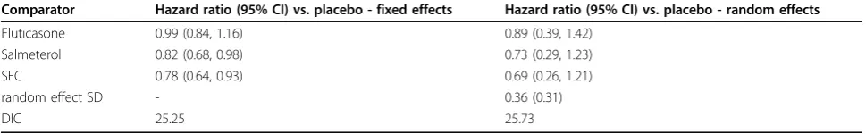
Results of the fixed and random effects models are pre-sented as Table 4. The results provide no evidence that
the random effects model is preferred; the DIC for the random effects model is marginally higher (lower DIC values are preferred, with differences of 2-5 considered important [19,20]) and the high level of uncertainty around the random effects standard deviation estimate indicates that there is little information to inform the random effect parameter.
Figure 1 provides a presentation of the uncertainty in the analysis, showing the probability that each treatment takes each possible ranking (1st best, 2nd best, etc). For example, the figure tells us that there is a very low prob-ability that fluticasone is the first or second most effica-cious treatment in this analysis and that there is a 56% probability that is the third best and a 42% probability that it is the worst treatment.
Again it must be noted that this example data set is not an appropriate basis for answering the clinical ques-tion of which is the most efficacious treatment with respect to the mortality endpoint.
Discussion
In this tutorial we have described how network meta-analysis can be conducted on the log-hazard ratio scale when the data on the survival endpoint available from the network of studies takes varying forms: count statis-tics and hazard ratio statisstatis-tics from two and multi-arm trials.
In highlighting the importance of network sis as an extension to conventional pairwise
meta-analy-sis Ades et al point out that “...to ignore indirect
evidence either makes the unwarranted claim that it is irrelevant, or breaks the established precept of systema-tic review that synthesis should embrace all available
evidence” [6]. A similar criticism can be levelled at
meta-analyses that omit data points on the basis of the summary measure reported. This may result in inten-tional or uninteninten-tional selection bias. Furthermore, even if separate analyses are conducted for each summary measure available, this may have undesirable conse-quences by: producing conflicting results; producing coherent results that would not be supported by an‘all
embracing’analysis; and unlinking some comparators
from the network entirely.
Other authors have presented methods for combining arm-based mean change from baseline data with contrast
Table 4 Network meta-analysis results
Comparator Hazard ratio (95% CI) vs. placebo - fixed effects Hazard ratio (95% CI) vs. placebo - random effects
Fluticasone 0.99 (0.84, 1.16) 0.89 (0.39, 1.42)
Salmeterol 0.82 (0.68, 0.98) 0.73 (0.29, 1.23)
SFC 0.78 (0.64, 0.93) 0.69 (0.26, 1.21)
random effect SD - 0.36 (0.31)
mean difference data [21] and for combining mean time, median time and count data within a parametric survival model [22]. Further research is required in this area, for example in to methods for combining incidence rate data with count data, as these summary measures are often reported interchangeably across trials.
Other approaches to combining alternative reporting of time to event data have been discussed [8,23-26], recommended [27] and implemented [28,29]. These approaches involve the approximation of the log hazard ratio and its variance using available count statistics. The methods used in this tutorial avoid the use of approximations, instead utilising cumulative count sta-tistics directly in the analysis.
A further common statistic reported for survival end-points is arm-specific median survival time. This data can be incorporated using a similar approach as for count data. A binomial likelihood is used to incorporate the number of subjects experiencing an event (half the number of patients) and the number of patients ana-lysed in to the model:
rs k, ~Bin F( s k, ,ns k, ) (19)
Note thatrs,kshould be calculated outside the model
to ensure it is a whole number. A log hazard for each
trial arm ln (hs,k) is then derived from the cumulative
failure probabilityFs,kand median survival timeTs,k:
ln( ) ln ln( , ) ,
,
h Fs k
Ts k s k =
− ⎛ ⎝
⎜⎜ ⎞⎠⎟⎟ (20)
The arm-specific log hazard estimates are then included in a treatment effect model that takes the same form as that for hazard ratio reporting multi-arm trials (see equation 14). It should be noted that analysis of median survival times requires the strong assumption of a constant hazard in each trial arm. The code for incor-porating median survival time data is also provided in the Appendix.
Where multiple statistics are reported for a trial, hazard ratio statistics should be used in preference to median survival time and count data as hazard ratio statistics incorporate information about time to event and censor-ing, and analysis of hazard ratio statistics does not require assumptions stronger than proportional hazards. If both median survival time and count data are reported, a judgement is required to weigh up the relative merits of each presentation, as median survival time incorporates information about censoring but its analysis requires the stronger assumption of constant hazards.
Finally, this tutorial discusses methods for running analyses on the log hazard ratio scale. However, the question of which is the most appropriate scale for a given analysis (the scale on which transitivity and exchangeability are most likely to hold) - is an empirical question. Further work is required to develop methods for selecting the most appropriate scale for a given data set.
Conclusions
Meta-analysis of summary statistics continues to play an important role in medical research [30,31]. Where only summary statistics are available, the analyst performing pairwise or network meta-analysis may be faced with multiple summary statistics for a given endpoint. We present methods for meta-analysing different statistics summarising survival data on the hazard ratio scale. By incorporating all data presentations in a single analysis, we avoid the potential selection bias associated with conducting an analysis for a single statistic only, and the potential difficulties of interpretation, misleading results and loss of available treatment comparisons associated with conducting separate analyses for different summary measures. The methods described also allow use of the most informative statistic available from each study.
Appendix - WinBUGS code
A) Fixed effects analysis model{
#Define Prior Distributions #On tx effect mean beta[1] < -0 for (tt in 2:nTx){ beta[tt]~dnorm(0,1.0E-6) }
#On individual study baseline effect for(ss in 1:nStudies){
alpha[ss] ~ dnorm(0,1.0E-6) }
#Fit data
#For hazard ratio reporting studies for(ii in 1:LnObs ){
Lmu[ii] < - alpha[Lstudy[ii]]*multi[ii] + beta[Ltx [ii]] - beta[Lbase[ii]]
Lprec[ii] < - 1/pow(Lse[ii],2)
Lmean[ii] ~ dnorm(Lmu[ii],Lprec[ii]) }
#For binary data reporting studies for(ss in 1:BnObs){
logCumHaz[ss] < - alpha[Bstudy[ss]] + beta[Btx [ss]] - beta[Bbase[ss]]
cumFail[ss] < - 1-exp(-1*exp(logCumHaz[ss])) Br[ss] ~ dbin(cumFail[ss], Bn[ss])
}
# Calculate HRs for (hh in 1:nTx) { hr[hh] < -exp(beta[hh]) }
# Ranking plot for (ll in 1:nTx) {
for (mm in 1:nTx) {
rk[ll,mm] < - equals(ranked(beta[],mm),beta[ll]) }
} } # Data
# Data set descriptors
list(LnObs = 5, BnObs = 8, nTx = 4, nStudies = 5) # Log hazard ratio and log hazard data
Lstudy[] Ltx[] Lbase[] Lmean[] Lse[] multi[]
1 1 1 0 0.066 1
1 2 1 0.055 0.063 1
1 3 1 -0.154 0.070 1
1 4 1 -0.209 0.072 1
2 2 1 -0.276 0.203 0
END
# Binary data
Bstudy[] Btx[] Bbase[] Br[] Bn[]
3 3 1 1 229
3 1 1 1 227
4 2 1 4 374
4 3 1 3 372
4 4 1 2 358
4 1 1 7 361
5 3 1 1 554
5 1 1 2 270
END # Initial values
list(alpha = c(-0.50,-0.50,-0.50,-0.50,-0.50), beta = c(NA,-0.5,-0.5,-0.5))
list(alpha = c(0.50,0.50,0.50,0.50,0.50), beta = c (NA,0.5,0.5,0.5))
B)Random effects analysis (changes required to incorporate random effect in bold)
model{
#Define Prior Distributions #on random tx effect variance sd~dunif(0,5)
reTau < - 2/pow(sd,2) #On tx effect mean beta[1] < -0 for (tt in 2:nTx){ beta[tt]~dnorm(0,1.0E-6) }
#On individual study baseline effect for(ss in 1:nStudies){
#Define random effect for (ss in 1:nStudies){
for(tt in 1:nTx){
re[ss,tt]~dnorm(0,reTau) }
} #Fit data
#For hazard ratio reporting studies for(ii in 1:LnObs ){
Lmu[ii] < - alpha[Lstudy[ii]]*multi[ii]+ re[Lstudy [ii],Ltx[ii]]
-re[Lstudy[ii],Lbase[ii]] + beta[Ltx[ii]] - beta [Lbase[ii]]
Lprec[ii] < - 1/pow(Lse[ii],2)
Lmean[ii] ~ dnorm(Lmu[ii],Lprec[ii]) }
#For binary data reporting studies for(ss in 1:BnObs){
logCumHaz[ss] < - alpha[Bstudy[ss]]+ re[Bstudy [ss],Btx[ss]]
-re[Bstudy[ss],Bbase[ss]] + beta[Btx[ss]] - beta [Bbase[ss]]
cumFail[ss] < - 1-exp(-1*exp(logCumHaz[ss])) Br[ss] ~ dbin(cumFail[ss], Bn[ss])
} # Calculate HRs
for (hh in 2:nTx) { hr[hh] < -exp(beta[hh]) }
# Ranking plot for (ll in 1:nTx) {
for (mm in 1:nTx) {
rk[ll,mm] < - equals(ranked(beta[],mm),beta[ll]) }
} }
# Data as for fixed effects analysis ############################ # Initial values
list(alpha = c(-0.50,-0.50,-0.50,-0.50,-0.50), beta = c(NA,-0.5,-0.5,-0.5),sd = 0.1)
list(alpha = c(0.50,0.50,0.50,0.50,0.50), beta = c (NA,0.5,0.5,0.5),sd = 1)
C) Additional code required for data reported as median survival times
for (ii in 1:medianNObs ){
medianMu[ii] < - alpha[medianStudy[ii]] + beta [medianTx[ii]]
-beta[medianBase[ii]]
prob[ii] < - exp(-median[ii]*exp(medianMu[ii])) medianR[ii] ~ dbin(prob[ii],medianN[ii]) }
Acknowledgements
James Roger and Oliver Keene are acknowledged for their valuable comments on the methods presented in this paper.
Author details
1Oxford Outcomes Ltd., Oxford, UK.2University of York, York, UK.
Authors’contributions
BW conducted the statistical analysis and drafted the manuscript. NH conceived the study and developed the winBUGS code. DAS contributed to the design of the study and drafting of the manuscript and validated the statistical analysis. All authors reviewed and approved the manuscript.
Competing interests
No specific funding was provided for the preparation of this manuscript. However, some of the methods presented were developed as part of an empirical project funded by GlaxoSmithKline.
Received: 9 May 2009 Accepted: 10 June 2010 Published: 10 June 2010
References
1. Caldwell DM, Ades AE, Higgins JPT:Simultaneous comparison of multiple treatments: combining direct and indirect evidence.BMJ2005, 331:897-900.
2. Ades AE:A chain of evidence with mixed comparisons: model for multi-parameter synthesis and consistency of evidence.Stat Med2003, 22(19):2995-3016.
3. Hasselblad V:Meta-analysis of multitreatment studies.Med Decis Making
1998,18:37-43.
4. Collett D:Modelling survival data in medical research., Second 2003, Chapman & Hall/CRC.
5. Kleinbaum DG, Klein M:Survival analysis: a self-learning text.Springer, U.S, Second 2005.
6. Ades A, Sculpher M, Sutton AJ, Cooper NJ, Abrams KR, Welton N, Lu G: Bayesian Methods for Evidence Synthesis in Cost-Effectiveness Analysis.
Pharmacoeconomics2006,24:1-19.
7. Chan AW, Hróbjartsson A, Haahr MT, Gøtzsche PC, Altman DG:Empirical evidence for selective reporting of outcomes in randomized trials: comparison of protocols to published articles.JAMA2004, 291(20):2457-65.
8. Parmar MKB, Torri V, Stewart L:Extracting summary statistics to perform meta-analyses of the published literature for survival endpoints.Stat Med1998,17:2815-34.
9. Whitehead A:Meta-Analysis of Controlled Clinical Trials.John Wiley and Sons: Chichester 2002.
10. Salanti G, Higgins JP, Ades AE, Ioannidis JP:Evaluation of networks of randomised trials.Stat Methods Med Res2008,17(3):279-301. 11. Baker WL, Baker EL, Coleman C:Pharmacologic treatments for chronic
obstructive pulmonary disease: a mixed-treatment comparison meta-analysis.Pharmacotherapy2009,29(8):891-905.
12. Boyd G, Morice AH, Pounsford JC, Siebert M, Peslis N, Crawford C:An evaluation of salmeterol in the treatment of chronic obstructive pulmonary disease (COPD).Eur Respir J1997,10:815-21.
13. Calverley P, Pauwels R, Vestbo J, Jones P, Pride N, Gulsvik A, Anderson J, Maden C, Trial of Inhaled Steroids and Long-Actingb2-Agonists (TRISTAN) Study Group:Combined salmeterol and fluticasone in the treatment of chronic obstructive pulmonary disease: a randomized controlled trial.
Lancet2003,361:449-56.
14. Celli B, Halpin D, Hepburn R, Byrne N, Keating ET, Goldman M:Symptoms are an important outcome in chronic obstructive pulmonary disease clinical trials: results of a 3-month comparative study using the breathlessness, cough, and sputum scale (BCSS).Resp Med2003,97(suppl A):S35-43.
15. Burge PS, Calverley PMA, Spencer S, Anderson JA, Maslen TK, on behalf of the ISOLDE Study Investigators:Randomised, double-blind, placebo-controlled study of fluticasone propionate in patients with moderate to severe chronic obstructive pulmonary disease: the ISOLDE trial.BMJ
16. Calverley PMA, Anderson JA, Celli B, Ferguson GT, Jenkins C, Jones PW, Yates JC, Vestbo J, for the TORCH Investigators:Salmeterol and fluticasone propionate and survival in chronic obstructive pulmonary disease.N Engl J Med2007,356:775-89.
17. Sin DD, Wu L, Anderson JA:Inhaled corticosteroids and mortality in chronic obstructive pulmonary disease.Thorax2005,60:992-7. 18. Lunn DJ, Thomas A, Best N, Spiegelhalter D:WinBUGS - a Bayesian
modelling framework: concepts, structure, and extensibility.Stat Comput
2000,10:325-337.
19. Spiegelhalter DJ, Best NJ, Carlin BP, Van der Linde A:Bayesian measures of model complexity and fit (with discussion).J R Stat Soc2002,64:1-34. 20. The BUGS project:DIC: Deviance Information Criterion.
[http://www.mrc-bsu.cam.ac.uk/bugs/winbugs/dicpage.shtml#q9], Accessed 10/02/2010. 21. Welton NJ:Mixed treatment comparisons: outcome measures. Lecture
notes from Indirect and Multiple Comparisons course.Leicester University 2008.
22. Welton NJ, Cooper NJ, Ades AE, Lu G, Sutton AJ:Mixed treatment comparison with multiple outcomes reported inconsistently across trials: Evaluation of antivirals for treatment of influenza A and B.Stat Med
2008,27:5620-39.
23. Ma J, Liu W, Hunter A, Zhang W:Performing meta-analysis with incomplete statistical information in clinical trials.BMC Med Res Methodol
2008,8(1):56.
24. Michiels S, Piedbois P, Burdett S, Syz N, Stewart L, Pignon JP:Meta-analysis when only the median survival times are known: a comparison with individual patient data results.Int J Technol Assess2005,21(1):119-25. 25. Tierney JF, Stewart LA, Ghersi D, Burdett S, Sydes MR:Practical methods
for incorporating summary time-to-event data into meta-analysis.Trials
2007,8:16.
26. Williamson PR, Tudur Smith C, Hutton JL, Marson AG:Aggregate data meta-analysis with time-to-event outcomes.Stat Med2002,21:3337-51. 27. Higgins JPT, Deeks JJ, (editors):Chapter 7: Selecting studies and collecting
data.Cochrane Handbook for Systematic Reviews of Interventions Version 5.0.0 (updated February 2008). The Cochrane CollaborationHiggins JPT, Green S 2008 [http://www.cochrane-handbook.org].
28. Green JA, Kirwan JM, Tierney JF, Symonds P, Fresco L, Collingwood M, Williams CJ:Survival and recurrence after concomitant chemotherapy and radiotherapy for cancer of the uterine cervix: a systematic review and meta-analysis.Lancet2001,358(8):781-86.
29. Langendijk JA, Leemans CR, Buter J, Berkhof J, Slotman BJ:The Additional Value of Chemotherapy to Radiotherapy in Locally Advanced Nasopharyngeal Carcinoma: A Meta-Analysis of the Published Literature.
J Clin Oncol2004,22(22):4604-12.
30. Lyman GH, Kuderer NM:The strengths and limitations of meta-analyses based on aggregate data.BMC Med Res Methodol2005,5(1):14. 31. Riley RD, Simmonds MC, Look MP:Evidence synthesis combining
individual patient data and aggregate data: a systematic review identified current practice and possible methods.J Clin Epidemiol2007, 60(5):431-9.
Pre-publication history
The pre-publication history for this paper can be accessed here: http://www.biomedcentral.com/1471-2288/10/54/prepub
doi:10.1186/1471-2288-10-54
Cite this article as:Woodset al.:Network meta-analysis on the log-hazard scale, combining count and log-hazard ratio statistics accounting for multi-arm trials: A tutorial.BMC Medical Research Methodology201010:54.
Submit your next manuscript to BioMed Central and take full advantage of:
• Convenient online submission
• Thorough peer review
• No space constraints or color figure charges
• Immediate publication on acceptance
• Inclusion in PubMed, CAS, Scopus and Google Scholar • Research which is freely available for redistribution
![Table 3 Log hazard statistics for a multi-arm trial (TORCH[16])](https://thumb-us.123doks.com/thumbv2/123dok_us/9320492.1919360/4.595.56.291.111.175/table-log-hazard-statistics-for-multi-trial-torch.webp)