Synchronization of Chaos in Nonlinear Finance System by means of Sliding Mode and Passive Control Methods: A Comparative Study

ISSN 1392–124X (print), ISSN 2335–884X (online) INFORMATION TECHNOLOGY AND CONTROL, 2015, T. 44, Nr. 2

Synchronization of Chaos in Nonlinear Finance System by means of Sliding

Mode and Passive Control Methods: A Comparative Study

Uğur Erkin Kocamaz

1*

_{, Alper Göksu}

2

_{, Harun Taşkın}

3

_{, Yılmaz Uyaroğlu}

4

1 _{Department of Computer Technologies, Vocational School of Karacabey,}

Uludağ University, 16700 Karacabey, Bursa, Turkey e-mail: [email protected]

2 _{Department of Industrial Engineering, Engineering Faculty,}

Sakarya University, 54187 Serdivan, Sakarya, Turkey e-mail: [email protected]

3 _{Department of Industrial Engineering, Engineering Faculty,}

Sakarya University, 54187 Serdivan, Sakarya, Turkey e-mail: [email protected]

4 _{Department of Electrical & Electronics Engineering, Engineering Faculty,}

Sakarya University, 54187 Serdivan, Sakarya, Turkey e-mail: [email protected]

http://dx.doi.org/10.5755/j01.itc.44.2.7732

Abstract. In this paper, two different control methods, namely sliding mode control and passive control, are investigated for the synchronization of two identical chaotic finance systems with different initial conditions. Based on the sliding mode control theory, a sliding surface is determined. A Lyapunov function is used to prove that the passive controller provides global asymptotic stability of the system. Numerical simulations validate the synchronization of chaotic finance systems with the proposed sliding mode and passive control methods. The synchronization performance of these two methods is compared and discussed.

Keywords: Chaotic finance system, chaos synchronization, sliding mode control, passive control.

1. Introduction

Financial system dynamics have a significant role in micro- and macroeconomics [6, 10, 39]. The financial and economic systems become more complicated and economic growth changes from low to high financial markets. Based on multiple variables, the process of economical development and growth is more complex. They have some nonlinear factors such as interest rate, the price of goods, investment demand, and stock [25]. Even if an economical system possesses deterministic characteristics, a chaotic behaviour can occur in the financial system. Chaotic systems have sensitive dependence on initial conditions. Because of slight errors, chaotic dynamical systems can lead to completely different trajectories. Hence, the synchronization of chaos in the financial systems is required. It has great importance from the management point of view to avoid undesirable trajectories and

make the precise economic adaptation and prediction possible.

control. This method provides discontinuous control by enforcing the system states to stay on the sliding surface [19]. Recently, the sliding mode control has been used to synchronize many chaotic systems [14, 21, 29]. Nowadays, applying the synchronization using only one state controller is preferred due to its considerable significance in reducing the cost and complexity [33, 37]. The passive control method has been gaining importance in synchronization and control of chaotic systems on account of using only a single controller. The main idea of passivity theory is to keep the system internally stable with implementing a controller which renders the closed loop system passive upon the properties of the system. In recent years, the passive control method has been successfully implemented for the synchronization of hyperchaotic Lorenz [31], unified [32], Rikitake [34], and other chaotic systems. The methodology of sliding mode and passive control is studied in many papers [14, 19, 21, 29, 31, 32, 34].

In the last decade, some chaotic finance systems were introduced [3, 8, 25]. The dynamic behaviours of the chaotic finance systems such as equilibrium points, stability, topological structure, Lyapunov exponents and Hopf bifurcation analysis were investigated in detail [1, 10, 25–27, 38, 39]. The control of the chaotic finance systems was implemented with effective speed feedback control [5, 8, 35, 38], linear feedback control [5, 30, 35, 38], adaptive control [5], the selection of gain matrix control [35], the revision of gain matrix control [35], passive control [9], and time-delayed feedback control [6, 11, 39] methods. The control of fractional-order chaotic finance system has been realized using a sliding mode control method [7]. Active controllers [17, 40], nonlinear feedback controllers [4, 16], adaptive controllers [15], and a single controller based on Lyapunov stability theory and linear matrix inequality [20] are employed for synchronizing the chaotic finance systems. To the knowledge of the authors, neither sliding mode control nor passive control approach for the synchronization of the chaotic finance systems exist in the literature.

In this study, further investigations on the synchronization of chaotic finance system have been explored. First, a brief description of the chaotic finance system is given. Then, sliding mode controllers are employed for achieving the synchronization of two identical chaotic finance systems. Based on the property of passivity theory, a single passive controller

is designed for synchronization of this nonlinear system. Afterwards, numerical simulations are performed for the synchronization of the chaotic finance systems to show the effectiveness of the proposed sliding mode and passive control methods. Finally, the advantages and disadvantages are discussed.

2. Chaotic Finance System

Financial systems consist of enterprise units and markets that interact, generally in a complex manner, for the purpose of economic growth within investment and the demand of commercials. In this study, the considered finance model defines the time variations of three state variables: x is the interest rate, y is the investment demand, and z is the price exponent. The interest rate is the amount charged, expressed as a percentage of principal by a lender to a borrower for the use of assets. Investment demand can be defined as the desired or planned capitals and inventories by the firms. It has a negative relation between investment expenditures and the interest rate. Price exponent determines the variance of the price distribution. The chaotic finance system is described by the set of three first-order differential equations as follows

cz x z

x by y

x a y z x

  

  

  

  

, 1

, ) (

2 ₍₁₎

where a, b, c are positive constant parameters, and represent the saving amount, the per-investment cost, and the elasticity of demands of commercials, respectively [25]. In a financial system, saving amount means that enterprise unit increases its gross financial. Per-investment cost is defined as the ratio of original cost less distribution received from target funds. The elasticity of demands of commercials is a measure of the relationship between a change in the quantity demanded of a particular good and a change in its price. The nonlinear finance system exhibits chaotic behaviour when the parameter values are taken as

a = 0.9, b = 0.2, and c = 1.2 [35]. The time series of the chaotic finance system under the initial conditions

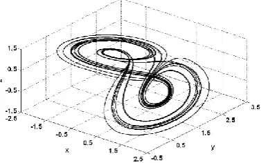
x(0) = 1, y(0) = 2, and z(0) = –0.5 are shown in Fig. 1, the 2D phase portraits are shown in Fig. 2, and the 3D phase plane is shown in Fig. 3.

Figure 2. Phase portraits of chaotic finance system in (a) x–y phase plane, (b) x–z phase plane, (c) y–z phase plane

Figure 3. 3D phase plane of chaotic finance system

3. The Synchronization of Chaotic Finance

Systems using Sliding Mode Control

The parameters a, b and c are taken in a range to ensure the system (1) will display chaotic behaviour. In order to observe the synchronization, it is assumed that two chaotic finance systems are taken where the drive system controls the response system. The initial position on the drive system is different from that of the response system. The drive system is denoted by subscript 1 and the response system is denoted by subscript 2. The drive system is given by:

, , 1 , ) ( 1 1 1 2 1 1 1 1 1 1 1 cz x z x by y x a y z x             (2)

and the response system is defined as:

) ( ), ( 1 ), ( ) ( 3 2 2 2 2 2 2 2 2 1 2 2 2 2 t u cz x z t u x by y t u x a y z x                (3)

where u1(t), u2(t), and u3(t) in Eq. (3) are the sliding

mode control functions to be determined. The drive system is subtracted from response system to obtain the control function for synchronization. The e1, e2,

and e3 state errors between finance system (3) that is

to be controlled and the controlling finance system (2) are defined as

. , , 1 2 3 1 2 2 1 2 1 z z e y y e x x e       (4)

Thus, the error dynamics become

). ( ), ( ), ( 3 3 1 3 2 2 1 2 2 2 2 1 1 1 2 2 1 3 1 t u ce e e t u x x be e t u y x y x ae e e                  (5)

The error dynamics (5) can be regularized in matrix notation as

u y x Ae

e ( , ) (6)

where , 0 ) , ( , 0 1 0 0 1 0 2 1 2 2 1 1 2 2                            

 x x

y x y x y x c b a A  . ) ( ) ( ) ( 3 2 1            t u t u t u u (7)

According to the sliding mode control methodology, the control signal u is defined as [29]:

) ( ) , ( )

(t x y Bvt

u   (8)

where v is a control signal, and B is a matrix. B is chosen so that (A, B) will be controllable. Therefore, B

is taken as

. 0 1 1            B (9)

substituted into Eq. (6), the system alters to the following linear form:

,

Bv Ae

e  (10)

where nxn

R

A , BRnxm , eRn , and vRm .

The error dynamics of system (10) are separated into two subsystems and one of them includes a control signal. In order to transform the system into its regular form, a non-singular transformation can be used as follows:

,

Te

z (11)

where T is a non-singular transformation matrix. When Eq. (11) is substituted into the linear form (10), the following alternative system, which consists of two subsystems, is revealed as

, , 2 22 1 21 2 2 12 1 11 1 Lv z A z A z z A z A z        (12)

where L is a gain matrix. Then, the sliding surface design is considered as

, 0 )

(t SzS1z1S2z2

s (13)

where 1( ) 1

m n x

R

S   , and S₂R1 . oolving for z1 in

Eq. (13) and substituting z1 into Eq. (12) yields

, ] [ _{11 12 2} 1 _{1 1}

1 A A S S z

z    (14)

which renders the ideal sliding motion. oince the dynamics of z2 depend on z1, the stabilization of z1

stabilizes z2. According to the dynamics of z1, the

eigenvalues of the expression A11 – A12S2–1S1 should be

in the left-half s-plane so that the dynamics of z1 are

asymptotically stable. In order to find S2–1S1, pole

replacement and optimal control techniques can be used. S2 may be arbitrary selected on condition that it

is not singular. After that, S1 is calculated according to

S2. Now, the sliding surface equation becomes

. )

(t Sz STe Ce

s    (15)

This implies

. ST

C (16)

The eigenvalues of A11 – A12S2–1S1 have been

placed in the left-half s-plane. Then S2–1 has been

selected as identity matrix and so S1 is calculated [12].

From Eq. (16), the sliding surface vector C has been determined as [–1.75 2.75 0]. Then, the sliding mode state equation gives asymptotically stable behaviour, when the sliding mode variable is designed as



1.75 2.75 0



e 1.75e1 2.75e2. Ce

s     (17)

From the property of the sliding mode control theory [14]:



( ) sign( )



. )

( )

(t CB 1C kI Ae q s

v     (18)

where k and q are the sliding mode control parameters. A large value of k can cause chattering; an appropriate value of q reduces chattering and the time to reach the sliding surface.

Now, the v(t) control signal becomes

  



1.75( ) 1 2.75( ) 2

)

(t k ae k be

v ). 75 . 2 75 . 1 ( sign 75 .

1 e3q  e1 e2 (19) Then, the required sliding mode control signal is obtained as Eq. (8) where (e) and B are described as

in Eqs. (7) and (9), respectively:

. 0 ) ( ), ( ) ( ), ( ) ( 3 2 1 2 2 2 1 1 2 2 1         t u t v x x t u t v y x y x t u (20)

The synchronization of chaotic finance system (3) by using the sliding mode control method is completed with Eqs. (19) and (20). Hence, the synchronization of two identical chaotic finance systems by means of sliding mode control is achieved.

4. The Synchronization of Chaotic Finance

Systems using Passive Control

The drive system is again taken to be:

, , 1 , ) ( 1 1 1 2 1 1 1 1 1 1 1 cz x z x by y x a y z x             (21)

and the response system is defined as:

2 2 2 2 2 2 2 2 2 2 2 , 1 ), ( ) ( cz x z x by y t u x a y z x              (22)

where u(t) in Eq. (22) is the passive control function to be determined. As in the sliding mode control, the drive system is subtracted from response system to obtain the synchronization error. Then,

3 1 3 2 1 2 2 2 2 1 1 2 2 1 3 1 , ), ( ce e e x x be e t u y x y x ae e e                (23)

where e1, e2, and e3 are the state errors and system (23)

is called the error system.

One term of system (23) can be written as

. ) ( ) )(

( _{1 2 1 2 1 2 1}

2 1 2

2 x x x x x x x e

x      

 (24)

oo, error system (23) can be rewritten in the following form: . , ) ( ), ( 3 1 3 1 2 1 2 2 1 1 2 2 1 3 1 ce e e e x x be e t u y x y x ae e e                (25)

The purpose is to determine the passive controller

u(t) for stabilizing error system (25) at a zero equilibrium point. By assuming that the state variable

e1 is the output of the system and supposing Y = e1, Z1

= e2, Z2 = e3, z = [Z1 Z2]T, then system (25) can be

). ( , , ) ( 1 1 2 2 2 2 2 2 1 1 1 t u y x y x aY Z Y cZ Y Z Y x x bZ Z                (26)

The passive control theory has the following generalized form [31]:

, ) , ( ) , ( , ) , ( ) ( 0 u Y Z a Y Z b Y Y Y Z p Z f Z       (27)

and according to system (26):

. 1 ) , ( , ) , ( , 1 ) ( ) , ( , ) ( 1 1 2 2 2 2 1 2 1 0                         Y Z a y x y x aY Z Y Z b x x Y Z p cZ bZ Z f (28)

As in [31], let the storage function is chosen as

), ( 2 1 ) ( ) ,

(Z Y W Z Y2

V   (29)

where ( )

2 1 )

( 22

2 1 Z

Z Z

W   is a Lyapunov function

of f0(Z) with W(0) = 0. Then,

Y Y Z p Z Z W Z f Z Z W Y Y Z Z Z W Y Z V dt d ) , ( ) ( ) ( ) ( ) ( ) , ( 0 _            . ) , ( ) ,

(Z Y Ya Z Y u

Yb 

 (30)

According to Eq. (28), by taking the derivative of

W(Z)





. ) ( ) ( ) ( ) ( 2 2 2 1 2 1 2 1 0 cZ bZ cZ bZ Z Z Z f Z Z W Z W dt d Z W                  (31)

oince W(Z)0 and W(Z)0 , it can be concluded that W(Z) is the Lyapunov function of

) (

0 Z

f and that f0(Z) is globally asymptotically

stable [34]. The controlled system (25) is equivalent to a passive system and can be asymptotically globally stabilized at its zero equilibrium by the following state feedback controller [32]:





v Y Z x x y x y x aY v Y x x Z Z y x y x aY Z v Y Y Z p Z Z W Y Z b Y Z a t u T                                     _{ }           1 2 1 1 1 2 2 2 1 2 1 1 1 2 2 2 1 1 ) ( 1 ) ( ) ( 1 ) , ( ) ( ) , ( ) , ( ) ( (32)

where α is a positive constant, and v is an external input signal. By noting Z1 = e2, Z2 = e3 and Y = e1

conversions, the passive control function becomes

. )

( )

(t ae1 x2y2 x1y1 x1 x2 e2 e1 v u        (33)

The synchronization of chaotic finance system (22) by using the passive control method is completed with Eq. (33). Therefore, the synchronization of two identical chaotic finance systems by means of passive control is achieved.

5. Numerical simulations

In this section, numerical simulations are performed using MATLAB™ to demonstrate the synchronization of two identical chaotic finance systems. The fourth-order Runge–Kutta method with fixed step size being equal to 0.001 is used to simulate the system. The parameter values of nonlinear finance systems are taken as a = 0.9, b = 0.2, and c = 1.2 to ensure chaotic behaviour [35]. The initial values are chosen as x1(0) = 1, y1(0) = 2, z1(0) = –0.5, x2(0) = –1,

y2(0) = 1.7, z2(0) = 0.5. For reducing the chattering, the

sliding mode control coefficient q is considered as 0.1.

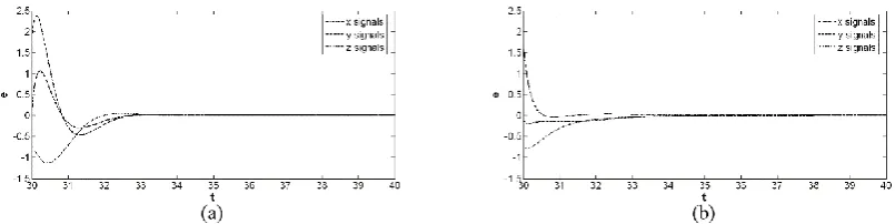
The passive control coefficient v is needed for controlling a chaotic system to its non-zero equilibrium points. oince the synchronization is stabilizing the errors between drive and response system towards to zero, v has to be 0. In order to determine the proper values of k and α control coefficients, they are varied from 1 to 7 with 2 increments. Figs. 4 and 5 show the synchronization error signals for k and α coefficients when the controllers are activated at t = 25.

As seen in Figs. 4 and 5, when the sliding mode coefficient k and the passive control coefficient α are greater then 1, the synchronization errors are not changing so much. Bigger k and α choices give slightly better results, but they can cause some difficulties in realization. As a consequence, k and α coefficients are taken as 5 in the simulations. When the sliding mode controllers and the passive controller are activated at t

Figure 4. The effect of k coefficient to synchronization errors when the sliding mode controllers are activated at t = 25 (a) e1 signals, (b) e2 signals, (c) e3 signals

Figure 5. The effect of α coefficient to synchronization errors when the passive controller is activated at t = 25 (a) e1 signals, (b) e2 signals, (c) e3 signals

Figure 7. The time response of states for synchronization of chaotic finance systems with the controllers are activated at t = 25 (a) x signals, (b) y signals, (c) z signals

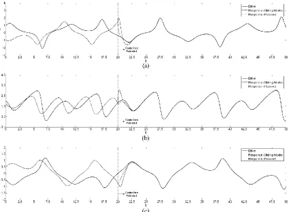
Figure 9. The time response of the error signals for synchronization of chaotic finance systems with the controllers activated at t = 20 (a) sliding mode controllers, (b) passive controller

Figure 10. The time response of the error signals for synchronization of chaotic finance systems with the controllers activated at t = 25 (a) sliding mode controllers, (b) passive controller

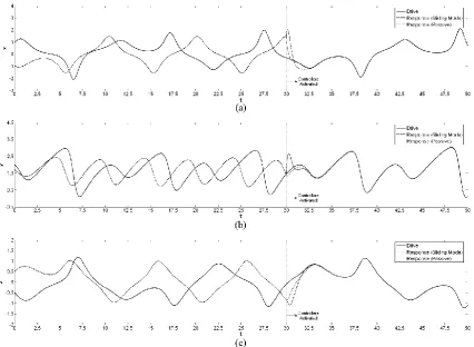
Figure 11. The time response of the error signals for synchronization of chaotic finance systems with the controllers activated at t = 30 (a) sliding mode controllers, (b) passive controller

As expected, the related Figs. 6–8 outputs show that both the sliding mode controllers and the passive controller have achieved synchronization of chaotic finance systems with an appropriate time period. The error signals that are shown in Figs. 9–11 converge asymptotically to zero. The figures include compara-tive results for the synchronization of chaotic finance systems. While synchronization is provided at t ≥ 24 by using the sliding mode control, it is reached when t

≥ 28 with the passive control when the controllers are activated at t = 20. Also, the synchronization is first observed with the sliding mode controllers when the controllers are activated at t = 25, and t = 30. Therefore, these comparisons show that the sliding mode control method performs better than the passive control method for the synchronization of two identical chaotic finance systems. The sliding mode control method realizes the synchronization using two controllers while the passive control method requires only one controller. Multiple controllers appear to reduce the synchronization time period, whereas a single controller provides simplicity in implemen-tation.

The passive control method achieves synchroni-zation by adding or subtracting a value only to the interest rate which is dependent on the saving amount, interest rates and investment demands. It does not need any changes in the investment demand and price exponent, so it is simpler to implement. On the other hand, sliding mode control method achieves synchro-nization by altering the interest rate and investment demand. It calculates the quantity of changes by using the saving amount, per-investment cost, interest rates, investment demands and price exponents. Both methods do not require the elasticity of demands of commercials for synchronization. The sliding mode control method appears to have some advantages in synchronization speed, but by comparison with the passive control, it is more difficult to apply.

6. Conclusions

factors of demand and volume changes. They lead to nonlinearity in a system. oynchronization to the global finance system utilizes some benefits to economic growth on account of obtaining the same interest rate, investment demand and price exponent. Also, it can reduce the asymmetrical economic risks.

Based on sliding mode and passive control theory, two sliding mode controllers and a single passive controller have been designed for synchronization of chaos in two identical chaotic finance systems. Numerical simulations show all the theoretical analyses of the proposed control methods are succeeded in synchronizing the two chaotic financial systems. oliding mode controllers regulate the synchronization of chaotic finance systems more effectively than the passive controller in all cases that are shown in Figs. 6–11, so the sliding mode method is more appropriate. The advantage of the passive control method is to achieve the synchronization of chaotic finance systems with only one controller which provides simplicity in implementation. While the sliding mode control realizes synchronization by altering the interest rate and investment demand, the passive control only alters the interest rate.

Acknowledgments

We would like to present our thanks to anonymous reviewers for their helpful suggestions.

References

[1] B. N. Ao. The research on financial chaos control based on dynamic theory. Int. Conf. on Computer Science and Network Technology, ICCSNT, Harbin, China, 2011, Vol. 4, pp. 2478–2481.

[2] S. Benitez, L. Acho. Impulsive synchronization for a new chaotic oscillator. International Journal of Bifurcation and Chaos, 2007, Vol. 17, No. 2, 617– 623.

[3] G. L. Cai, J. J. Huang. A new finance chaotic attractor. International Journal of Nonlinear Science, 2007, Vol. 3, No. 3, 213–220.

[4] G. L. Cai, M. Z. Yang. Globally exponentially attractive set and synchronization of a novel three-dimensional chaotic finance system. Third Int. Conf. on Information and Computing, ICIC, Wuxi, Jiangsu, China, 2010, Vol. 2, pp. 70–73.

[5] G. L. Cai, H. J. Yu, Y. X. Li. Stabilization of a modified chaotic finance system. Fourth Int. Conf. on Information and Computing, ICIC, Phuket, Thailand, 2011, pp. 188–191.

[6] W. C. Chen. Dynamics and control of a financial system with time-delayed feedbacks. Chaos, Solitons & Fractals, 2008, Vol. 37, No. 4, 1198–1207. [7] S. Dadras, H. R. Momeni. Control of a

fractional-order economical system via sliding mode. Physica A-Statistical Mechanics and Its Applications, 2010, Vol. 389, No. 12, 2434–2442.

[8] J. Ding, W. Yang, H. Yao. A new modified hyperchaotic finance system and its control.

International Journal of Nonlinear Science, 2009, Vol. 8, No. 1, 59–66.

[9] S. Emiroglu, Y. Uyaroglu, E. Koklukaya. Control of a chaotic finance system with passive control. 3rd International Symposium on Sustainable Development, Sarajevo, Bosnia and Herzegovina, 2012, pp. 125–130. [10] Q. Gao, J. H. Ma. Chaos and Hopf bifurcation of a finance system. Nonlinear Dynamics, 2009, Vol. 58, No. 1-2, 209–216.

[11] H. Gelberi, S. Emiroglu, Y. Uyaroglu, M. A. Yalcin. Time delay feedback control of chaos in a hyper chaotic finance system. 3rd _{Int. Symp. on Sustainable} Development, Sarajevo, Bosnia and Herzegovina, 2012, pp. 139–144.

[12] F. Gouaisbaut, M. Dambrine, J. P. Richard. Robust control of delay systems: A sliding mode control design via LMI. System & Control Letters, 2002, Vol. 46, No. 4, 219–230.

[13] J. M. V. Grzybowski, M. Rafikov, J. M. Balthazar. Synchronization of the unified chaotic system and application in secure communication. Communications in Nonlinear Science and Numerical Simulation, 2009, Vol. 14, No. 6, 2793–2806.

[14] Y. Y. Hou, B. Y. Liau, H. C. Chen. Synchronization of unified chaotic systems using sliding mode controller. Mathematical Problems in Engineering, 2012, Vol. 2012, Article 632712.

[15] A. Jabbari, H. Kheiri. Anti-synchronization of a modified three-dimensional chaotic finance system with uncertain parameters via adaptive control. International Journal of Nonlinear Science, 2012, Vol. 14, No. 2, 178–185.

[16] J. G. Jian, X. L. Deng, J. F. Wang. Globally exponentially attractive set and synchronization of a class of chaotic finance system. 6th _{Int. Sym. on Neural} Networks, Wuhan, China, Advances in Neural Networks – Lecture Notes in Computer Science, 2009, Vol. 5551, 253–261.

[17] S. O. Kareem, K. S. Ojo, A. N. Njah. Function projective synchronization of identical and non-identical modified finance and Shimizu–Morioka systems. Pramana – Journal of Physics, 2012, Vol. 79, No. 1, 71–79.

[18] U. E. Kocamaz, Y. Uyaroglu. Non-identical synchronization, anti-synchronization and control of single-machine infinite-bus power system via active control. Information Technology and Control, 2014, Vol. 43, No. 2, 166–174.

[19] K. Konishi, M. Hirai, H. Kokame. Sliding mode control for a class of chaotic systems. Physics Letters A, 1998, Vol. 245, No. 6, 511–517.

[20] J. Li, C. R. Xie. Synchronization of the modified financial chaotic system via a single controller. Int. Conf. on Frontiers of Manufacturing Science and Measuring Technology, ICFMM2011, Chongqing, China, Advanced Materials Research, 2011, Vol. 230, No. 1, 1045–1048.

[21] C. L. Li, K. L. Su, L. Wu. Adaptive sliding mode control for synchronization of a fractional-order chaotic system. Journal of Computational and Nonlinear Dynamics, 2013, Vol. 8, No. 3, 031005. [22] C. L. Li, Y. N. Tong. Adaptive control and

[23] A. G. Lukyanov, V. I. Utkin. Methods of reducing equations for dynamic-systems to a regular form. Automation and Remote Control, 1981, Vol. 42, No. 4, 413–420.

[24] R. Z. Luo, Y. L. Wang, S. C. Deng. Combination synchronization of three classic chaotic systems using active backstepping design. Chaos, 2011, Vol. 21, No. 4, Article 043114.

[25] J. H. Ma, Y. S. Chen. Study for the bifurcation topological structure and the global complicated character of a kind of nonlinear finance system(I). Applied Mathematics and Mechanics, 2001, Vol. 22, No. 11, 1240–1251.

[26] J. H. Ma, Y. Q. Cui, L. X. Liu. Hopf bifurcation and chaos of financial system on condition of specific combination of parameters. Journal of Systems Science & Complexity, 2008, Vol. 21, No. 2, 250–259. [27] C. Ma, X. Y. Wang. Hopf bifurcation and topological

horseshoe of a novel finance chaotic system. Communications in Nonlinear Science and Numerical Simulation, 2012, Vol. 17, No. 2, 721–730.

[28] J. W. Sun, Y. Shen, Q. Yin, C. J. Xu. Compound synchronization of four memristor chaotic oscillator systems and secure communication. Chaos, 2013, Vol. 23, No. 1, Article 013140.

[29] V. Sundarapandian, S. Sivaperumal. Global chaos synchronization of hyperchaotic Chen system by sliding mode control. International Journal of Engineering Science and Technology, 2011, Vol. 3, No. 5, 4265–4271.

[30] Y. Uyaroglu, R. Temel, H. Kirlioglu. Feedback control of chaos in a hyperchaotic finance system. 3rd Int. Symp. on Sustainable Development, Sarajevo, Bosnia and Herzegovina, 2012, pp. 135–138. [31] F. Q. Wang, C. X. Liu. Synchronization of

hyperchaotic Lorenz system based on passive control.

Chinese Physics, 2006, Vol. 15, No. 9, 1971–1975. [32] F. Q. Wang, C. X. Liu. Synchronization of unified

chaotic system based on passive control. Physica D: Nonlinear Phenomena, 2007, Vol. 225, No. 1, 55–60. [33] G. M. Wang. Stabilization and synchronization of Genesio-Tesi system via single variable feedback controller. Physics Letters A, 2010, Vol. 374, No. 28, 2831–2834.

[34] X. J. Wu, J. S. Liu, G. R. Chen. Chaos synchronization of Rikitake chaotic attractor using the passive control technique. Nonlinear Dynamics, 2008, Vol. 53, No. 1-2, 45–53.

[35] M. Yang, G. Cai. Chaos control of a non-linear finance system. Journal of Uncertain Systems, 2011, Vol. 5, No. 4, 263–270.

[36] H. T. Yau, Y. C. Pu, S. C. Li. Application of a chaotic synchronization system to secure communication. Information Technology and Control, 2012, Vol. 41, No. 3, 274–282.

[37] W. G. Yu. Synchronization of three dimensional chaotic systems via a single state feedback. Communications in Nonlinear Science and Numerical Simulation, 2011, Vol. 16, No. 7, 2880–2886. [38] H. J. Yu, G. L. Cai, Y. X. Li. Dynamic analysis and

control of a new hyperchaotic finance system. Nonlinear Dynamics, 2012, Vol. 67, No. 3, 2171– 2182.

[39] R. Y. Zhang. Bifurcation analysis for a kind of nonlinear finance system with delayed feedback and its application to control of chaos. Journal of Applied Mathematics, 2012, Vol. 2012, Article 316390. [40] X. S. Zhao, Z. B. Li, S. A. Li. Synchronization of a

chaotic finance system. Applied Mathematics and Computation, 2011, Vol. 217, No. 13, 6031–6039.