The Use of the Lambert Function Method for Analysis of a Control
System with Delays
Irma Ivanovienė
Kaunas University of Technology, Department of Applied Mathematics, Studentu st. 50, LT-51368, Kaunas, Lithuania
e-mail: [email protected]
Jonas Rimas
Kaunas University of Technology, Department of Applied Mathematics, Studentu st. 50, LT-51368, Kaunas, Lithuania
e-mail: [email protected]
http://dx.doi.org/10.5755/j01.itc.42.4.2484
Abstract. The mathematical model of the mutual synchronization system with complete graph structure, composed of 𝑛 (𝑛 ∈ 𝑁) oscillators, is investigated. This mathematical model is defined by the matrix differential equation with delayed argument. The solution of the matrix differential equation with delayed argument is obtained by applying the Lambert W function method. On the base of this solution, the step responses matrix of the synchronization system is defined and the transients in the system are investigated. The results of calculations, received by the Lambert function method, the dde23 method in Matlab and the exact method of consequent integration, are compared.
Keywords: synchronization system; differential equations; delayed argument; Lambert function.
1. Introduction
Control systems and engineering techniques have become an integral part of modern technology. These systems are often components added to other complex systems to increase their functionality or to meet the set of design criteria. Usually they are being investigated by applying their mathematical models. More exact analysis of the systems demands the use of the more complicated mathematical models. Often the delays of the signals, transferred along the control system, must be included into these models. The delays make the investigation of the model more cumbersome. Usually investigation of such model demands solution of delay differential equation. The principal difficulty in solving delay differential equation lies in its special transcendental character. The characteristic equation of linear delay differential equation is transcendental and has infinite number of roots. For solution of this characteristic equation in the present work we use a method based on the application of Lambert W functions. The Lambert W functions for analytic investigations of various dynamical systems with delays were applied by
several authors [1–5]. In [1, 2], the new analytic approach to obtain the complete solution for systems of delay differential equations based on the concept of Lambert W function is presented. In [3], Yi et al. have considered the problem of feedback controller design via eigenvalue assignment for systems of linear delay differential equations using Lambert W function method. In [4], the approach of using the Lambert W functions to time domain analysis of a class of fractional order time delay systems is extended. In [5], a survey on analysis of delay systems via Lambert W function is given. In all these works the systems of differential equations of order not greater then third were investigated by applying the Lambert W function method.
2. Formulation of the problem
In the presented work, the multidimensional control system with delays and with structure of complete graph is investigated. The mathematical model of this system is the matrix differential equation with delayed argument [6–9]
), ( = ) ( ) ( )
(t B1x t B2x t zt
x′ + + −t (1)
,0],
[
),
(
=
)
(
t
φ
t
t
∈
−
t
x
where
(
)
Tn t x t x t x t
x()= 1() 2() () is the desired
vector function, 𝑇(here and in what follows) denotes
the operation of transposition, 𝜏 is a constant time
delay,
φ
(
t
)
is a vector–valued preshape (initial)function,
z
(
t
)
is a free term (continuous functiondepending on the initial conditions), 𝜅 is a coefficient,
1
B and B2 are 𝑛×𝑛 (𝑛 ∈ 𝑁) numerical matrices
(
B B ∈Rn×n)
2
1, , , = 1 E
B
κ
(2),
1
=
2B
n
B
−
κ
(3) 0 1 1 1 1 1 1 1 0 1 1 1 1 1 0 1 1 1 1 1 0 = B (4)(
E
∈
R
n×n is the identity matrix, matrixB
∈
R
n×noutlines the structure of the internal links of the system).
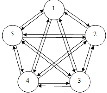
As an example of a control system, described by the equation (1), the mutual synchronization system of the communication network, having structure of the
complete graph and composed of 𝑛 oscillators, can be
pointed out [8] (in Fig. 1 the scheme of the internal links of the system, composed of 5 oscillators, is presented). In this case, the symbol xi(t) in (1) stands for the phase of the 𝑖–th oscillator.
Figure 1. The scheme of internal links of the system, when 𝑛= 5
We shall assume that
≤
+
+
∫
0;
if
,
0,
>
if
,
)
(
=
)
(
0 0 0 0t
x
t
f
t
x
d
f
t
x
i i i i t ix
x
(5)here x0i =xi(0) (i=1,n) is the initial phase of the
𝑖–th oscillator’s oscillation, f (t)
i is the frequency of
the 𝑖–th oscillator,
i
f0 is the own frequency (the
frequency of the 𝑖–th oscillator when the control
signal is disconnected). The meaning of (5) is the
following: the control signal to the 𝑖–th oscillator at
time 𝑡= 0 is connected up. Before this time moment
the 𝑖–th oscillator works with its own frequency
i
f0 . Taking into account (5), we get the following expressions for the initial vector function
φ
(
t
)
and the free vectorz
(
t
)
of (1):,
)
)
(
)
(
)
(
(
=
)
(
t
φ
1t
φ
2t
φ
nt
Tφ
(6),0], [ , 1, = , = )
( 0 0
t
φ
i t f it+xi i n t∈ − (7).
)
(
=
)
(
01 02 0 Tn
f
f
f
t
z
(8)3. Solution of the matrix differential equation
with delayed argument
If to apply the Lambert W function method (see [10], p. 23), the solution of (1) on the interval
[
0,+∞)
can be expressed as follows:
=
)
(
=
)
(
( ) = 0 =x
x
xd
z
C
e
C
e
t
x
Sk t kk t k t k S k
′
+
∞ − −∞ ∞ −∞∫
∑
∑
∑
+
− ∞ → k t k S N N k NC
e
=lim
=
lim
( )(
)
;
=
0
x
x
x
d
z
C
e
Sk t k N N k N t
′
+
− − ∞ →∑
∫
(9)here
C
k is a 𝑛× 1 coefficient matrix–columncomputed from the given preshape function
)
(
=
)
(
t
t
x
φ
, which is an initial state of delaydifferential equation (1) for
t
∈
[
−
t
,0]
, andC
k′
is a𝑛×𝑛 coefficient matrix computed from the given free
term
z
(
t
)
of the matrix differential equation (1)(procedures of calculation of these matrices are explained in [1], p. 222 and [2], p. 2434). In the
computations of the solution
x
(
t
)
we shall use theapproximate expression, obtained from (9) at fixed and finite
𝑁
:. ) ( = ) ( ( ) = 0 =
x
x
x d z C e C e t x k t k S N N k t k t k S N N k ′ + + − − −∫
∑
4. The step responses matrix of the system
A good representation about transients in the system can be obtained by determining its responses to perturbations having form of the unit jump [6]. The
response of the 𝑖–th oscillator’s oscillation phase to a
unit jump in the
j
–th oscillator’s oscillation phase weshall call the step response
h
ij(
t
)
. The set of the step responses hij(t)(
i,j=1,n)
forms 𝑛×𝑛 matrix(
())
= )
(t h t
h ij (the step responses matrix of the
synchronization system). We shall find the matrix
)
(
t
h
.When the increment of the phase of the 𝑗–th
oscillator takes form of the unit jump, the increment of the free term of the equation (1) can be expressed as follows ; ) ( = )
(t t I(j)
z δ
∆ (11)
here
I
(j) is the matrix–column all entries of whichare zeros except the𝑗–th element, which is equal to
1
,𝛿(𝑡) is the Dirac delta function. Taking this into
account and using (1), we get the following differential equation for step responses
(
i
j
n
)
t
h
ij(
)
,
=
1,
of the system:, ) ( = ) ( ) ( )
( 1 2 ( )
j j
j
j t Bh t B h t t I
h′ + + −
t
δ
(12), 1, = n j
[
,0]
; 0,= )
(t t∈ −t
hj
here
(
)
Tnj j
j
j t h t h t h t
h ()= 1 () 2 () () is the 𝑗 –th
column of the step responses matrix
h
(
t
)
, matrices1
B and B2 are defined by (2) and (3), respectively. Firstly, we shall find the solution of (12) on the interval
[ ]
0,t
.Column–vector
h
j(
t
−
t
)
is a zero column–vectoron the interval
[ ]
0,t
due to the initial conditions (see (12)). Taking this into account on the interval[ ]
0,t
, we get the following system of differential equations for the step responsesh
ij(
t
),
i,j=1,n:(
)
≠ + . if 0, , = if ), ( = ) ( ) ( ' j i j i t t h thij ij
δ
κ (13)
Solution of (13) is the set of functions:
h
ij(
t
)
=
0
if
i
≠
j
and h (t)=e t1(t)ij
κ
− if
i
=
j
(i
,
j
=
1,
n
);here
1(
t
)
is the Heaviside step function.Using the solution of (13), the differential equation
(12) on the interval
[
t
,+∞)
can be presented ashomogeneous matrix delay–differential equation
, 1, = 0, = ) ( ) ( )
(t B1h t B2h t j n
h′j + j + j −t
(
() () ())
= (), =)
(t h1 t h2 t h t t
hj j j nj T jj (14)
[ ]
0,t ; ∈t
here 𝜑𝑗(𝑡) is the preshape vector–function. The
entries of the vector–function 𝜑𝑗(𝑡) assume the
following values:
(
)
≠ − . if 0, , = if ), 1( = ) ( = ) ( j i j i t e t t t i j ij κ j j (15)Applying the Lambert function method, the
solution of (14) on the interval
[
t
,+∞)
can beexpressed as follows [see [2], p. 2434]:
= ) ( = ) ( = j C e t h k t k S k j
∑
∞ −∞[
,)
; , 1, = ), ( lim = = +∞ ∈∑
− ∞→ e Ck j j n t
t
t k S N N k N (16) here , ) ( 1
= 1 1
2Te B B
W
Sk k − Bt −
t ) ( 1 2 t B k BTe
W − is the value of the 𝑘–th branch 𝑊𝑘(𝐻)
of the matrix Lambert function 𝑊(𝐻) at
t
1 2 = B TeB
H − , 𝐶𝑘(𝑗) are the complex–valued vectors
corresponding to the preshape vector–function 𝜑𝑗(𝑡)
(see (15)). The algorithms for finding Ck(j) and 𝑊𝑘 are explained in [2, p. 2434–2435]. From (16) the approximate expression for ℎ𝑗(𝑡) follows:
, 1, = ), ( = ) ( = n j j C e t h k t k S N N k j
∑
− (17)[
,+∞)
; ∈t
there 𝑁 is a sufficiently large natural number.
5. Investigating of stability
Analyzing the distribution of roots of the transcendental characteristic equation of delay system we can obtain information about its stability. Let’s write down the characteristic equation of investigated system and find out the closed form solution of it.
Let’s write down homogeneous differential equation corresponding to (1):
0, = ) ( ) ( )
( + 1 + 2 −
t
′t B xt B xt x,0].
[
),
(
=
)
(
t
φ
t
t
∈
−
t
x
(18)Assuming that a solution of homogeneous differential equation is a vector function
C e t
x()= St (19)
and substituting it into (18), we get the transcendental characteristic equation 0 = 2 1 t S e B B
S+ + − (20)
(here 𝑆 is 𝑛×𝑛 numerical matrix, 𝐶is a nonzero
solution of the homogeneous differential equation (18)
if matrix 𝑆 in its expression will be a root of the
transcendental characteristic equation (20). We shall find the closed form expression for roots of (20).
Multiplying both sides of (20) by
e
St, we get(
S B1)
e = B2.S −
+ −t (21)
Performing further transformations, we multiply both sides of (21) by
t
e
B1t. This yields(
)
= 1 .2 1 1 t t t
t
t
S B Be B e e B
S+ − −
Recall that the matrices B1 and B2 in equation (18)
commute. Then 𝑆 and B1 will commute as well (see,
for example, [10], p. 119). Taking this into account, we can write
(
)
(
)
= 1 .2 1 1
t
t
t
t
S B Be B e
B
S+ + − (22)
We know [12] that the Lambert W function is a function satisfying equality
. = )
(z e () z
W Wz
So, we can write
. = ) ( 1 2 ) 1 2 ( 1 2 t t t t t
t B W B eB B
e B e
e B
W − − − (23)
Equating (22) and (23), we obtain
(
)
= ( 1).2 1 t t t B e B W B S+ −
From this equality, we get the closed form expression for the roots of (20):
. ) (
1
= 1 1
2 e B B
W
S − t Bt −
t
Since the Lambert W function has an infinite number of branches, the matrix transcendental characteristic equation (20) will have an infinite number of roots, which can be expressed as follows:
, ) (
1
= W B2 e 1 B1
Sk k − B −
t t t (24)
.
2,
1,
0,
=
±
±
k
If matrix
t
1t2 = B eB
H − is diagonalizable, then we
compute the eigenvalues Λi, i=1,n of 𝐻 and the
corresponding eigenvector matrix𝑉. To each branch 𝑘
)
1,0,1,...,
,...,
=
(
k
−∞
−
+∞
of the Lambert Wfunction, we get:
(
(
),
(
),...,
(
)
)
.
diag
=
)
(
H
V
W
Λ
1W
Λ
2W
Λ
V
−1W
k k k k nIf 𝐻 is not diagonalizable, then 𝑊𝑘(𝐻) has more
complicated structure (see, for example, [17], p. 2125).
Having found matrix 𝑆𝑘 (
k
=
0,
±
1,
±
2,...
), wecalculate its eigenvalues
λ
k,i(
i
=
1,
n
)
. Analysis ofdistribution of these eigenvalues on the complex plane provides information about stability of the system (the system can be asymptotically stable, unstable or marginally stable [16]).
6. Comparing the Lambert function method
with the exact method of consequent
integration
The solutions of matrix delay differential equations (1) and (14) are presented by the infinite functional series (see (9) and (16)), which determines the exact solutions. In the real calculations we apply the approximate formulas (10) and (17), obtained from (9)
and (16) with finite 𝑁 (2𝑁+ 1 indicates the number
of branches of the Lambert W function, which are used in calculation of the solutions).
We shall investigate the rate of convergence of the approximate solutions of matrix delay–differential
equation (14) to its exact solution with increasing 𝑁.
For this purpose, we shall apply the exact expressions found by the method of consequent integration (method of “steps”) [8, 11].
We present the solution of (1), applying the Laplace transform, as follows [8]:
), ( ) ( ) ( 1 2 1 1 = p Z A e B A t
x pt l
d l − − −
∑
÷ (25);
1)
(
0
<
t
<
d
+
t
here = =( ) ,
1 p E
B pE
A − +κ
Z
(
p
)
÷
z
(
t
),
Z
(
p
)
isthe Laplace transform of the vector function
z
(
t
)
(sign
÷
links function with its Laplace transform),0,1,2,...
=
d
. Taking into account (2)–(4), we write), ( ) ( 1 1 ) ( 1 0 = p Z B e p n t
x pl l
l l d l t
κ
κ
− + + − ÷∑
t
1)
(
0
<
t
<
d
+
and , ) ( ) ( 1 1 = ) ( 1 1 0 = + − − + −
∑
e Z pp L B n t x pl l l l d l t κ κ (26)
;
1)
(
0
<
t
<
d
+
t
here L−1
(
F(p))
is the inverse Laplace transform of)
(
p
F
.Let’s write down the step responses matrix of the system. Using (1), (12) and (25), we obtain
,
)
(
1
1
))
(
(
=
)
(
1 0 = l pl l l d lij
e
B
p
n
t
h
t
h
tκ
κ
− ++
−
÷
∑
.
1)
(
0
<
t
<
d
+
t
{ }
−
×
−
∑
(
!
)
1
=
)
(
0
=
l
l
t
B
n
t
h
l ij
l l d
l ij
t
κ
),
1(
)
( t
t
κ
l
t
e
t l−
×
− −(27)
;
1)
(
0
<
t
<
d
+
t
here
{ }
ij l
B is the 𝑖𝑗–th entry of the matrix
B
l. Note,that (26) and (27) represent the exact expressions of the solutions on the interval (0,(d+1)t).
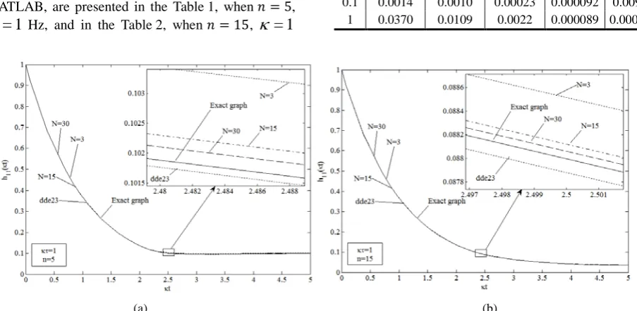
The step response h11(
κ
t) of mutualsynchronization system with a complete graph structure, computed by Lambert W function method
with different values of
N
and by the exact methodof consequent integration, are presented in Fig. 2. In this figure the graphs of the solutions, obtained by dde23 program in MATLAB, for the sake of comparison, are presented, as well.
The relative errors 𝛿 obtained at 𝜅𝑡= 2.5 (at mid
point of the interval
[0,5]
), using the Lambert Wfunction method with different values of 𝑁and the
numerical method based on the dde23 program in
MATLAB, are presented in the Table 1, when 𝑛= 5,
1
=
κ
Hz, and in the Table 2, when 𝑛= 15,κ
=
1
Hz. We can see from the tables, that, if 𝜏 is small
(𝜅𝑡 ≪1), then the results obtained by Lambert W
function method are more accurate if to compare them with the corresponding results got by the dde23 program in MATLAB. With an increase of the number
of oscillators 𝑛, the accuracy of the Lambert W
function method has tendency to increase.
Table 1. The relative error 𝛿 when 𝑛= 5
𝜿𝝉
LAMBERT
DDE23 𝑵
1 5 30 80
0.01 0.0000027 0.0000023 0.000013 0.0000054 0.0016
0.1 0.00083 0.00057 0.00013 0.000051 0.00019 1 0.017 0.0039 0.00075 0.00029 0.00092
Table 2. The relative error 𝛿 when 𝑛= 15
𝜿𝝉
LAMBERT
DDE23 𝑵
1 5 30 80
0.01 0.000045 0.000034 0.000023 0.0000092 0.0093 0.1 0.0014 0.0010 0.00023 0.000092 0.0092 1 0.0370 0.0109 0.0022 0.000089 0.00092
(a) (b)
Figure 2. Graphs of the step response ℎ11(𝜅𝑡) calculated by three methods: 1) the Lambert W function method with different values of 𝑁, 2) numerical method using dde23 program in MATLAB, 3) exact method of consequent integration (method of
“steps”)
7. Numerical results
7.1. Transients
For the calculation of the phase differences )
( )
(t x t
xi − j and the step responses hij(t), we have
applied the formulas (10) and (17), respectively, with
80 =
N (this means that we have used 161 branches of
the Lambert W function in the computations). On the base of the results in Section 6, the graphs of the transients, presented below, are sufficiently accurate
(in the presented figures these graphs practically coincide with the exact ones).
The calculations are performed assuming:
11,15 = 1999,
; 6,10 = 2001,
; 1,5 = 2003, = 0
i i i fi
κ
and
. i 0.6,
; i 0.3, = 0
even s i
odd s i
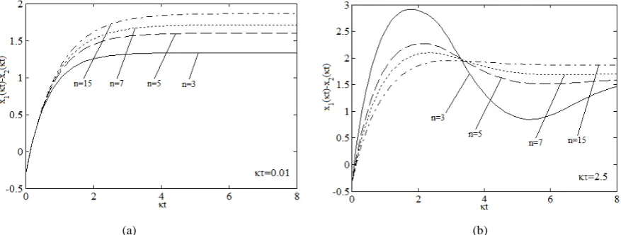
In Fig. 3 the graphs of the phase difference
) ( )
( 1
2 t x t
x − are given at different values of 𝜅𝜏 and for
different numbers of oscillators in the synchronization system with parameters of the system defined by (28). From the figure, we see that the character of the transients in the synchronization system crucially
depends on 𝑛 (the number of oscillators in the
synchronization system). If 𝑛= 3, the transients get
oscillatory features when 𝜅𝜏 ≥1, and with increase of
𝜅𝜏 the oscillatory features of the transients tend to
increase. If 𝑛= 15, the transients in the system go
without oscillatory features even when 𝜅𝜏= 2.5.
With an increase of 𝑛 and 𝜅𝜏 the duration of transients in the system changes insignificantly. In Fig. 4 the
graphs of the phase differences x1(t)−xj(t),
𝑗= 4,10,14 are presented.
(a) (b)
Figure 3. Graphs of the phase difference 𝑥1(𝑡)− 𝑥2(𝑡)
The graphs of some step responses are given in Fig. 5. The graphs presented on these figures show that the system under consideration is marginally stable since the step responses tend to positive finite
values when 𝜅𝑡 tends to infinity (the characteristic
equation of the system has simple zero root).
7.2. Stability
Analyzing the distribution of the eigenvalues of
matrices 𝑆𝑘 (𝑘= 0, ±1, ±2, …) (the roots of the
characteristic equation (20)) on the complex plane one can make a conclusion about system’s stability. In Fig. 6, the distribution of the eigenvalues λk,i(i=1,5)
of the matrices Sk(k=0,1,2) is presented on the
complex plane for the case 𝑛= 5 (the eigenvalues of
the matrices Sk(k=3,4,5,) are not shown here since they have greater in absolute value negative real parts and are located outside the drawing). From the figure
it follows that the right most eigenvalue is
λ
0,1. Thiseigenvalue is simple and has zero real part. This fact indicates that the system is marginally stable [16]. This conclusion coincides with the one obtained from the analysis of the graphs of step responses. In Fig. 7, the relation between real parts of eigenvalues
) 1,5 = (
0,i i
λ of matrix 𝑆0 and delay 𝜏 is presented.
Similar conclusions follow for other values of 𝑛.
Figure 4. Graphs of the phase differences 𝑥1(𝑡)− 𝑥𝑗(𝑡)
8. Conclusions
1. The Lambert function method is used for calculation of transients in the synchronization system, when the structure of the internal links in the system bear form of the complete graph. It is shown that using 161 branches of the Lambert W function
(taking N=80 ) in calculations of step responses
) ( t
hij κ , the relative error is not greater than 0.001 for
2.5 =
t
κ and n≤15 (here 𝑛 is the number of oscillators
in the synchronization system).
(a) (b)
Figure 5. Graphs of the step response h11(κt)
Figure 6. Distribution of eigenvalues λk,i(i=1,5) of matrices Sk(k=0,1,2) on the complex plane
Figure 7. Relation between real parts of eigenvalues
) 1,5 = (
0,i i
λ of matrix 𝑆0 and delay 𝜏
size, whereas time of calculation of transients by means of a method of consequent integration is in inverse proportion to the delay size.
3. The Lambert W function method has the advantage in comparison with a numerical method
based on the application of dde23 program in
MATLAB, if the product 𝜅𝜏 is small (𝜅𝜏 ≪1).
4. The method of research of dynamics, used in the presented work, can also be applied to other control systems, described by the linear matrix differential equations with delayed arguments and with commuting coefficient matrices.
References
[1] F. M. Asl, A. G. Ulsoy. Analysis of a system of linear delay differential equations. J. Dynamic Systems. Measurement and Control, 2003, Vol. 125, No. 2, 215–223.
[2] S. Yi, A. G. Ulsoy. Solution of a system of linear delay differential equation using the matrix Lambert function. In: Proceedings of the American Control Conference, Minneapolis, MN, 2006, pp. 2433–2438. [3] S. Yi, P. W. Nelson, A. G. Ulsoy. Eigenvalue
assignment for control of time delayed systems using the Lambert W function. Journal of Vibration and Control, 2010, Vol. 16, No. 7-8, 961–982.
[4] Y. C. Cheng, C. Hwang. Use of the Lambert W function for time-domain analysis of feedback fractional delay systems. IEE Proceedings online no.20050020 doi:10.1049/ip-cta:20050020, 2005. [5] S. Yi, P. W. Nelson, A. G. Ulsoy. Survey on Analysis
of Time Delayed Systems via the Lambert W Function.
DCDIS A Supplement, Advances in Dynamical Systems, 2007, Vol. 14(S2), 296–301.
[6] B. C. Kuo. Automatic control systems. 7-edition, Prentice-Hall, 1995.
[7] S. A. Bregni. A historical perspective on tele-communications network synchronization. IEEE Communications Magazine, 1998, Vol. 36, Issue 6, 158–166.
[8] J. Rimas. Investigation of the dynamics of mutually synchronized systems. Telecommunications and Radio Engineering, 1977, No. 32, pp. 68–79.
[10] S. Yi, P. W. Nelson, A. G. Ulsoy. Time-delay systems (analysis and control using the Lambert W function).
World Scientific, New Jersey, 2010.
[11] R. Bellman, K. L. Cooke. Differential-difference equations. Academic Press, New York, 1963.
[12] R. M. Corless, G. H. Gonnet, D. E. Hare, D. J. Jeffrey, D. E. Knuth. On the Lambert W function. Advances in Computational Mathematics, 1996, Vol. 5, 329–359.
[13] C. Coratheodary. Theory of functions of a complex variables. New York, 1954.
[14] R. Horn, C. Johnson. Matrix Analysis. Cambridge University Press, 1995.
[15] M. Malek-Zavarei, M. Jamshidi. Time-delay systems. North Holland, New York, 1987.
[16] M. Hirsh, S. Smale, R. Devaney. Differential equations, dynamical systems, and an introduction to chaos. Academic Press, 2012.
[17] E. Jarlebring, T. Damm.The Lambert W function and the spectrum of some multidimensional time delay systems. Automatica, 2007, Vol. 43, 2124–2128.