Use of Systems Analysis to Assess and Minimize
Water Security Risks
James Uber, Regan Murray, and Robert Janke
U. S. Environmental Protection Agency
UNIVERSITIES COUNCILON WATER RESOURCES
JOURNALOF CONTEMPORARY WATER RESEARCHAND EDUCATION
ISSUE 129, PAGES 34-40, OCTOBER 2004
D
rinking water systems are vulnerable tocontamination by toxic substances, whether the contaminants are introduced intentionally during a terrorist attack, or unintentionally through accidental cross-connections or backflow incidents. In this paper, we discuss the particular characteristics of distribution systems that make a “systems modeling” approach useful and effective in assessing, preventing, and mitigating water security threats, and we outline the research needed to develop robust models for water security.
Water Distribution Systems and the
Water Security Threat
Many characteristics of water distribution systems contribute to a systems-level complexity: the large spatial extent, multiple flow paths, and time and space varying flow rates. Conceptualizing this complexity is fundamental to understanding and minimizing water security risks.
Water distribution systems are spatially complex. Typically, they convey treated water to thousands or millions of customers spread across tens to hundreds of square kilometers through a looped (as opposed to a branched) network of pipes. Thus, there usually exist multiple flow paths between any set of “upstream-downstream” locations, with each path contributing a portion of the flow. Looped systems increase the reliability of the water supply through flow path redundancy, but also complicate network hydraulic and contaminant transport
behavior, which is dominated by the network topology and bulk water velocity.
Water distribution systems are also temporally complex. Water usage rates (demands) vary on hourly to monthly time scales. The ratio of peak hour to average system water demand over a one-day period varies from 3 to 6 (Haestad Methods, 2003). Most utilities use distribution system storage tanks to equalize demand, thereby economically satisfying the wide range of usage rates. Treated water is pumped to storage at a more-or-less constant rate, and excess demand or supply is accommodated by fluctuating stored volume. Thus, flow rates are time and space varying, and flow directions frequently reverse, corresponding to changes in pumping policy or water usage rates (e.g., storage tanks that were filling begin to drain, and vice-versa).
System Vulnerability and Network Flows. Source waters—rivers, reservoirs, and groundwater supplies—are vulnerable to intentional contamination because they are open and unsecured, and dilution by large flow rates and volumes will likely limit public health effects or require extremely large contaminant volumes. The impact of contamination at the water treatment plant intake or a unit process is also limited by dilution, since maximum flow occurs at the plant, and treatment processes themselves may also create a barrier for some contaminants. Distribution systems may also be vulnerable to intentional contamination, though the level of vulnerability would be system-specific.
Can distribution system flows support high concentrations of contaminants? The following contaminant mass balance equation describes the relationship between the concentration of the
introduced contaminant (contaminant source), Cs,
the contaminant volumetric flow rate, Qs, and the
distribution system pipe flow rate, Qp, and diluted
(in-situ) concentration, Cp,
, ⎟⎟
⎠ ⎞ ⎜ ⎜ ⎝ ⎛ =
p s s p
C C Q
Q or(1)
Note that there is an inverse relationship between
the pipe flow rate and the pipe concentration. If Cp
represents a concentration of health concern for downstream consumers–for example, the concentration such that an average adult drinking one liter has a 50% chance of developing illness
(ID50),
C
50p , or the concentration at which no adverseeffects are expected to be observed
(NOAEL),
C
NOAELp , then one can derivecontaminant-specific bounds on the pipe flow rates that could deliver such a dose:
(
)
(
)
⎟
⎟
⎠
⎞
⎜
⎜
⎝
⎛
≤
≤
⎟
⎟
⎠
⎞
⎜
⎜
⎝
⎛
50 50
50
max
min
p s s p
p s s
C
C
Q
Q
C
C
Q
(2)
The above bounds should represent reasonable minimum and maximum values, given uncertainty in
the various factors, and
C
pID
50(
W
/
L
)
50
=
×
, where W is the assumed body mass in kg and L is one liter.
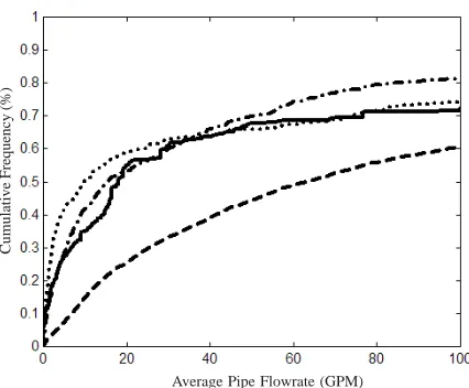
Pipe flow rate statistics, thus, can be used as a reasonable indicator of the vulnerability of distribution systems to contamination. Figure 1 shows the cumulative frequency of the temporally averaged pipe flow rates for four different operating systems (the plots are truncated at 100 gpm to highlight detail at the smaller flow rates). (These four systems were not subject to any form of pre-screening, and we did not analyze any other systems.) Note that between 60 and 80% of the average pipe flow rates are less than 100 gpm.
If security is a concern, the potential of health impacts from an intentional contamination by a given contaminant can be interpreted by computing the
above Q50p bounds. For a given contaminant, we
assumed
0
.
1
≤
Q
s≤
1
(gpm), 109 ≤Cs ≤1011(cells/L), 103 ≤ID50 ≤105(cells/Kg) or, for a 70Kg
body weight, 7x10⁴ ≤C50p ≤7x10⁶(cells/L),
which together yield maximum pipe flow bounds,
6 50
10
4
.
1
14
≤
Q
p≤
x
(gpm).The above pipe flow rate bounds show that, in the worst case, all four distribution systems may be vulnerable to contamination, as the upper bounds
onQ50p are large compared to, say, the 50th
percentile values of between 10 and 60 gpm. In this case, there remains a significant fraction (30-60%) of pipes with a flow rate less than the lower bound. We caution that this analysis is rough; it only indicates the potential for significant health consequences without fairly assessing their likelihood or severity.
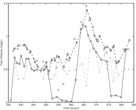
Storage Tanks, Flow Path Travel Times, and Contaminant Detection. Travel time characteristics in distribution networks affect the transport of contaminants from source to consumer, the robustness of contaminant detection schemes, and the post-detection time window for effective protection of public health. Time series of water quality indices, like those for free chlorine residual shown in Figure 2 reveal the importance of travel time characteristics. Figure 2 shows the variation in free chlorine residual at four distribution system sampling locations at one Midwest utility. These data show that the free chlorine residual can exhibit significant variability on hourly time scales, due in part to the loss of process control at the treatment plant, and in part to the interaction between travel time and chlorine decay kinetics. Chlorine decay kinetics combined with large storage tank residence Figure 1. Cumulative frequency of pipe average volumetric flow rates in four distribution systems.
s s p
pC QC
Q =
Cumulative Frequency (%)
time leads to large free chlorine loss within storage. When such tanks drain as a function of demand variation or system operation, low chlorine residual concentrations sweep across the storage tank service area, and any particular location experiences significant temporal variation in chlorine residual. More precisely, these locations are supplied at different times by distinct sets of flow paths having disparate travel time characteristics: a long travel time set that includes the storage tank, and a short travel time set that excludes it.
A comprehensive understanding of travel time characteristics in typical distribution systems requires system simulation. Here, we simulated “water age” using models of three utility distribution systems. Water age at a location is an integrated measure related to path travel time: it is the volume-weighted average of all travel times, over all paths leading back to a water source (where the age is zero). Typically, water age is simulated as a zero-order reaction with unit reaction rate coefficient. We used this standard approach, but we also prepared simulations where all water in storage used a zero reaction rate coefficient to highlight the role of storage tanks in travel time variation. In this modified approach, any water entering a tank stopped “growing old” until it left the tank and again entered the distribution system.
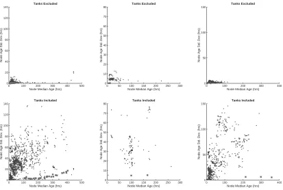
Water age histograms for the three networks are presented in Figure 3, and graphs of node water age statistics are presented in Figure 4. The latter figure is a scatter plot of water age standard deviation, at each location, versus its median value. These same
statistics are also calculated for the water stored in each tank, and they appear as squares to distinguish them from consumer nodes. In each figure, graphs on the left side exclude the effects of storage tanks on travel time, while those on the right correspond to the same network but include the effects of storage.
The water age statistics show consistent trends: storage tanks increase significantly the median water age throughout the network, and dramatically increase water age variability. Indeed, if it were not for storage tanks, the seemingly common perception that distribution systems are relatively static, save for slow (seasonal) fluctuations in water quality, might be close to correct. The large volume of finished water stored in tanks, combined with relatively small replacement rates, leads to high water ages in storage. The contrast between high age water in storage, and low age water delivered from the plant (when tanks are filling), is the source of large variability in water age and travel times.
The water age statistics relate approximately to the time available prior to consumption of contaminated water. A significant fraction of water delivered to consumers—perhaps up to one half of the total—arrives from the source within 24 hours. Yet a significant fraction of water requires days of travel time, due primarily to flow paths that involve storage tanks. These data provide at least order-of-magnitude time constraints on contaminant detection and emergency response. Near complete protection from intentional contamination may require rapid detection and emergency response within hours, but protection of a significant population fraction may still be possible days after contamination. We caution that these observations are a rough guide; in addition to being system specific, they ignore chemical and microbiological processes, proximity of population to contaminant source, disease pathology and treatment, and time varying flow paths and travel times.
Real distribution systems exhibit variability in travel time at all locations, and thus in water quality metrics affected by chemical or biochemical reaction kinetics. A travel time standard deviation on the order of days should be expected within the service area of a storage tank. If not treated carefully, such variability can affect the robustness of contaminant detection systems, specifically the frequency of false positive and negative events. is just beginning, but one Figure 2. Chlorine concentration variations over time at four
regulatory sampling locations in a Midwest utility.
335 340 345 350 355 360 365 370 375 380 385 0
0.5 1 1.5
Time (hours)
Figure 3. Water age frequency histograms for distribution systems 1 (left), 2 (center), and 3 (right). The travel time impacts of storage tanks are excluded from histograms on the left, and included on the right.
100 200 300 400 500 0
0.05 0.1 0.15 0.2 0.25 0.3 0.35 0.4 0.45 0.5
Age (hrs)
Frequency (%)
Tanks Excluded
100 200 300 400 500 0
0.05 0.1 0.15 0.2 0.25 0.3 0.35 0.4 0.45 0.5
Age (hrs)
Frequency (%)
Tanks Included
50 100 150 200 250 300 0
0.05 0.1 0.15 0.2 0.25
Age (hrs)
Frequency (%)
Tanks Excluded
50 100 150 200 250 300 0
0.05 0.1 0.15 0.2 0.25
Age (hrs)
Frequency (%)
Tanks Included
50 100 150 200 250 300 350 400 0
0.05 0.1 0.15 0.2 0.25 0.3
Age (hrs)
Frequency (%)
Tanks Included
50 100 150 200 250 300 350 400 0
0.05 0.1 0.15 0.2 0.25 0.3
Age (hrs)
Frequency (%)
Tanks Excluded
0 100 200 300 400 0
50 100 150
Node Median Age (hrs)
Node Age Std. Dev (hrs)
Tanks Excluded
0 100 200 300 400 0
50 100 150
Node Median Age (hrs)
Node Age Std. Dev. (hrs)
Tanks Included
0 50 100 150 200 250 300 0
10 20 30 40 50 60 70 80
Node Median Age (hrs)
Node Age Std. Dev (hrs)
Tanks Excluded
0 50 100 150 200 250 300 0
10 20 30 40 50 60 70 80
Node Median Age (hrs)
Node Age Std. Dev. (hrs)
Tanks Included
0 100 200 300 400 500 0
20 40 60 80 100 120 140
Node Median Age (hrs)
Node Age Std. Dev (hrs)
Tanks Excluded
0 100 200 300 400 500 0
20 40 60 80 100 120 140
Node Median Age (hrs)
Node Age Std. Dev. (hrs)
Tanks Included
straightforward approach involves on-line sensors that measure broad water quality indices, coupled with simple statistical measures of signal excursions from the expected value. Indeed, one existing sensor that could be used measures free chlorine, relying on its sensitivity as a sentinel to distribution system contamination. The large variation in normal free chlorine residual may, however, require large signal excursion thresholds to avoid false positives, and it may also reduce the effectiveness of such simple statistical warning alarms.
beginning, but one straightforward approach involves on-line sensors that measure broad water quality indices, coupled with simple statistical measures of signal excursions from the expected value. Indeed, one existing sensor that could be used measures free chlorine, relying on its sensitivity as a sentinel to distribution system contamination. The large variation in normal free chlorine residual may, however, require large signal excursion thresholds to avoid false positives, and it may also reduce the effectiveness of such simple statistical warning alarms.
The Role of Systems Analysis and
Simulation in Safeguarding Water
Supplies
Systems analysis and simulation enable an integrated analysis of the distribution system, bringing the spatial and temporal complexities together into a flexible modeling framework. Systems analysis can be used to understand the interdependencies of these complexities, and thus to aid decision-making in the operations of the system, and in the emergency response to contamination incidents. Network hydraulic models coupled with water quality models can be used to simulate threat scenarios to assess the potential impacts of contamination, and to design and pre-plan for mitigation strategies.
To adequately simulate water security contamination scenarios, many improvements to current modeling capabilities are needed. These improvements fall in two categories: improvements to the basic models and algorithms and improvements to application methods. Algorithms are needed that better reflect the following physical and chemical processes: mechanisms behind contaminant adherence to pipe walls; contaminant interactions with disinfectant residuals, disinfectant byproducts,
and corrosion products; particles and biological agents transport ; and the true time-dependent flow characteristics (Uber 2004a). In addition, basic research is needed to gain a better understanding of biofilms and their role in protecting contaminants from disinfection.
Application to Networks. In the post-9/11 environment, vulnerability assessments of water utilities are considered highly sensitive and are not widely shared. Distribution system networks may contain specific information that should not be in the public realm. (For a general discussion of securing publicly available geospatial data, see Baker, 2004.) For researchers to improve modeling capabilities, however, it is essential for them to have access to a broad variety of network data. There are at least two solutions to this problem. First, methods could be developed to transform networks visually so that they cannot be readily identified. Second, a database of “prototype” networks could be fabricated, adequately reflecting the hydraulics and water quality characteristics of real systems, but not representative of any single existing system.
Probabilistic Applications for Quantifying System Vulnerability. Because one cannot predict the behavior of terrorists, an assessment of the vulnerability of a drinking water system to intentional contamination must consider a large number of possible threat scenarios, or a threat ensemble (Murray 2004). These scenarios may include factors such as the type of contaminant, the concentration and quantity of the contaminant, and the location of contaminant introduction. System vulnerability then is based on an assessment of the entire threat ensemble. It is not obvious, however, what constitutes a sufficient ensemble. How can one determine the minimal number of scenarios that should be simulated to obtain an accurate assessment of a system’s vulnerability to contamination?
Network/Population Avg % Received Avg % Received Worst Case Received
Nonzero Dose Concentration Concern Concentration
of Concern of Concern
1 (< 10,000) 99% 17% 54%
2 (> 100,000) 75% 1% 4%
3 (>100,000) 60% 1% 6%
Table 1. Results from Monte Carlo analysis of three water distribution systems showing the average percentage of the population receiving a non-zero contaminant concentration or an LD50 concentration at the service connection. The last column lists the worst case exposure scenario.
behavior of certain contaminants in water, including chemical and biological warfare agents, and their impacts on humans from ingestion or other exposure routes. For contagious diseases, dynamic models of disease transmission must be developed to assess impacts accurately.
Applications for Assessing and Mitigating Threats. Table 1 shows the results of the probabilistic application of a hydraulic and water quality model to three distribution systems to estimate the likely health impacts from a terrorist contamination of a water distribution system. For each network, between 100 and 1,500 scenarios were simulated. Though the contaminant was the same for each scenario, other parameters were varied to reflect the uncertainty in the execution of the contamination. For each scenario, a 55-gallon drum of contaminant was introduced into the system, resulting flow paths and exposures were analyzed, and statistics were generated and examined. The contaminant was assumed to behave like a tracer and to be resistant to chlorine residuals, or to quickly deplete the residuals.
Preliminary results show that this approach has the potential to help water utilities assess the contaminants to which they are most vulnerable, identify the most vulnerable regions of their distribution systems, and select the most appropriate mitigation strategies for their system. The results in Table 1 show that the same scenario applied to various networks can have quite different outcomes, thus the unique physical and flow-dependent features of each distribution system weigh heavily on health outcomes. However, the simulations show that “on average” a low percentage of the population will be severely impacted by contamination events (1-17%). If particular nodes are protected, the vulnerability of the entire system can be dramatically reduced.
Applications for Contaminant Monitoring, Detection, and Warning. Early warning systems consisting of online sensors, remote communication devices, and data analysis tools are thought to hold great promise in protecting drinking water supplies from contamination. Probabilistic applications can be used to simulate early warning system responses to contamination and to test real-time early warning system components under realistic conditions. Algorithms can be developed to optimize the location of sensors to achieve various goals, such as the minimization of public health impacts (Uber 2004b). Many basic questions about the feasibility of early warning systems remain unanswered and realistic simulations of early warning systems would help to optimize their design and to determine how long a utility has to respond after detection of the contamination.
Such systems level models could ultimately serve as emergency response simulators that could train and test operators in their ability to rapidly respond to contamination events. Applications of models could also be used to design intervention strategies, such as the closure of valves to isolate portions of the network, or the superchlorination or decontamination of pipes. Improved models would enable the more accurate prediction of the spread of contaminant as well as its decay due to chlorine residual or treatment/decontamination.
Summary and Conclusions
particularly vulnerable to contamination are presented and discussed. In addition, the utility of a systems modeling approach in assessing, preventing, and mitigating water security threats is discussed. Research needs for better models and application capabilities are highlighted.
Author Bio and Contact Information
JAMES UBER is an Associate Professor of Environmental Engineering at the University of Cincinnati and is also with the Water Security Team at the USEPA National Homeland Security Research Center. He received a B.S. degree in Civil Engineering from Bradley University in 1983, and the M.S. and Ph.D. degrees in Environmental Engineering in 1985 and 1988 from the University of Illinois at Urbana-Champaign. His research interests are focused on the prediction and control of water quality in water distribution networks, and on general techniques for optimal planning and design of environmental systems. Address: Dept. Civil & Env. Eng., PO Box 210071, University of Cincinnati, Cincinnati, OH 45221; e-mail address: [email protected].
REGAN MURRAYis a Mathematical Statistician for the U. S. EPA’s National Homeland Security Research Center. Her research focuses on modeling of distribution systems, and the fate and transport of contaminants. She received a Bachelor of Arts from Kalamazoo College in 1994, and PhD in Applied Mathematics from the University of Arizona in 1999. Address: U.S. EPA HQ, 1200 Pennsylvania Ave, NW (8801R), Washington, DC 45220; e-mail address: [email protected]
ROBERT JANKEhas been with U.S. EPA, National Homeland Security Research Center, Office of Research and Development in Cincinnati, Ohio since June 2003, working on the Water Security Systems Modeling Program. Prior to joining EPA. As Team Leader for the Fernald cleanup, he helped in the completion of multiple, multi-million dollar Records of Decision and was instrumental in the design, construction, and deployment of a real-time radiological instrumentation program that helped shorten the soil cleanup schedule and significantly reduce costs. Rob has a Master of Science degree in Health Physics and a Bachelor of Science degree in Chemistry from the University of Cincinnati. Address: 26 West Martin Luther King Dr., Mail Stop 163, Cincinnati, Ohio 45268; e-mail address: [email protected]
References
Baker, John et al. 2004. Mapping the Risks: Assessing the Homeland Security Implications of Publicly Available Geospatial Information. The RAND Corporation.
Haestad Methods. 2003. Advanced Water Distribution Modeling and Management. Waterbury, CT: Haestad Press.
Murray, Regan, Robert Janke, and Jim Uber. 2004. The Threat Ensemble Vulnerability Assessment Program for Drinking Water Distribution System Security. Proceedings of EWRI Congress, Salt Lake City, UT. June, 2004.
Uber, James, Lewis Rossman, and Feng Shang. 2004. Extensions to EPANET for the fate and transport of multiple interacting chemical or biological components. Proceedings of EWRI Congress, Salt Lake City, UT. June, 2004.