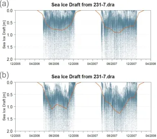
Sea ice draft in the Weddell Sea, measured by upward looking sonars

The United States Supreme Court held that the admission, at ajoint trial, of an unavailable codefendant's confession implicating the other codefendant, violates the right

Principals  support  ongoing  investigation  and  evaluation  of  diverse  teacher  education  models  and   practical  experience  placements,  including

In cases of severe thiamine deficiency, however, a broad enzymatic deficiency encompassing all three mitochondrial TPP- dependent enzymes would be expected to result in symptoms

For establishments that reported or imputed occupational employment totals but did not report an employment distribution across the wage intervals, a variation of mean imputation

see P ISANY -F ERRY , S APIR , V ERON & W OLFF , supra note 2, at 10, and ECB, Opinion of November 27, 2012 on the proposal for a Council Regulation entrusting the

While since then the SCADA data have been refined (i.e the measurements points have a lower uncertainty), and some of the models have been re-factored for offshore conditions, the

The proposed Center for Statistics and Application in Forensic Evidence (CSAFE) is a National Institute for Standards and Technology (NIST) sponsored national center of excellence