The impacts of data constraints on the predictive performance of a general process-based crop model (PeakN-crop v1.0)

(1)

www.geosci-model-dev.net/10/1679/2017/ doi:10.5194/gmd-10-1679-2017

The impacts of data constraints on the predictive performance of a

general process-based crop model (PeakN-crop v1.0)

Silvia Caldararu1,a, Drew W. Purves1, and Matthew J. Smith1

1_{Microsoft Research, Cambridge, UK}

a_{now at: Max Planck Institute for Biogeochemistry, Jena, Germany}

Correspondence to:Matthew Smith ([email protected])

Received: 17 September 2016 – Discussion started: 18 October 2016

Revised: 24 March 2017 – Accepted: 27 March 2017 – Published: 20 April 2017

Abstract. Improving international food security under a changing climate and increasing human population will be greatly aided by improving our ability to modify, understand and predict crop growth. What we predominantly have at our disposal are either process-based models of crop physiology or statistical analyses of yield datasets, both of which suf-fer from various sources of error. In this paper, we present a generic process-based crop model (PeakN-crop v1.0) which we parametrise using a Bayesian model-fitting algorithm to three different sources: data–space-based vegetation in-dices, eddy covariance productivity measurements and re-gional crop yields. We show that the model parametrised without data, based on prior knowledge of the parameters, can largely capture the observed behaviour but the data-constrained model greatly improves both the model fit and reduces prediction uncertainty. We investigate the extent to which each dataset contributes to the model performance and show that while all data improve on the prior model fit, the satellite-based data and crop yield estimates are particularly important for reducing model error and uncertainty. Despite these improvements, we conclude that there are still signif-icant knowledge gaps, in terms of available data for model parametrisation, but our study can help indicate the neces-sary data collection to improve our predictions of crop yields and crop responses to environmental changes.

1 Introduction

Improving food security is one of the greatest challenges currently facing humanity (Schmidhuber and Tubiello, 2007; Rosegrant and Cline, 2003). The increasing and developing

human population is driving up food demand and changing demand patterns. This is occurring alongside increasing an-thropogenic threats to supply, such as climate change. Pre-dicting and understanding how crops respond to changes in their environment through the use of mathematical models are needed to help address such threats, enabling advanced warning of potential threats and predictions of what alter-ations to agricultural practices might help prevent or mitigate problems. A continual challenge when developing models is knowing the generality of their predictions, either applied to multiple crops or across different space scales and timescales (Rosenzweig et al., 2014). Having one model to cover all cir-cumstances is obviously unrealistic, as are tailor-made mod-els to every conceivable circumstance. Thus, a challenge in developing models to help address the current food secu-rity crisis is identifying those that can be said to be gener-ally useful over particular scales of application. In the cur-rent study, we present a proof of concept that such an aim can be reached through using a process-based crop model (PeakN-crop v1.0), parametrised to available data using a model-fitting algorithm.

(2)

de-scribe growth phases specific to a particular crop type within their formulation. However, it is also partly because of the difficulty in developing generally applicable process-based crop models; it can be unclear which aspects of the model formulation can be said to be general versus crop specific and obtaining data to assess model generality continues to be a challenge. Some studies have avoided making crop-specific models by using broad crop categories such as C3 and C4 crops, based on the functional plant type concept (Bondeau et al., 2007; Osborne et al., 2015). Other models group a fam-ily of crop-specific parametrisations into a single framework, which limits generality but does facilitate use across different scales and crops (Brisson et al., 2003; Stackle et al., 2003).

Statistical crop models aim to capture relationships be-tween various predictor variables and crop properties without using any information of how such factors should be related from biology or ecology. For example, studies have predicted crop yields based on observed simple relationships between yield data and climate inputs (Lobell et al., 2011; Lobell and Field, 2007; Schlenker and Roberts, 2009); these have then been used to help understand past long-term trends in yields at large spatial scales and to make forward projections under climate change scenarios. Often, statistical models are devel-oped to be generally applicable to multiple crops and applied over multiple space scales and timescales, as these do not need to include any plant-specific concepts.

Both the process-based and statistical approaches have their disadvantages when it comes to obtaining general in-sights. Process-based models have often only been shown to be applicable at the individual field scale, making it un-clear if their predictions might provide information about crop responses at larger spatial scales. Process-based mod-els can also be sensitive to chosen parameter values and for-mulation, which has rarely been identified as applicable over multiple crop types or locations (Challinor et al., 2009). Sta-tistical models are limited by the extent to which the rela-tionships they capture are useful in predicting crop proper-ties outwith the circumstances that they have been verified for. This becomes a particularly important limitation given that one of the leading questions being addressed in food security is how different crops might grow in environments and under circumstances that we have not yet observed. For example, correlative models based on mean annual values of environmental variables are unlikely to capture the im-pacts of changes in extreme weather events or increases in atmospheric CO2, which have been shown to be essential to

understanding changes in crop yield under climate change (Porter and Semenov, 2005; Deryng et al., 2014). Further-more, simple statistical analyses rarely incorporate informa-tion on management agricultural practices such as planting and harvest dates, irrigation and fertiliser application, which account for a large proportion of variations in yield across the globe (Calvino et al., 2003; Zwart and Bastiaanssen, 2004).

An alternative to the extremes of either purely process-based or purely statistical crop models is to apply statistical

methods to process-based models to data constrain their pa-rameters. This technique, which is increasingly used in Earth system and vegetation modelling studies (Fox et al., 2009; Raupach et al., 2005), involves allowing some parameters to have undefined values and inferring those values by com-paring the model predictions to data; hence, the technique is called parameter inference or inverse modelling. The specific methods used vary but the aim is often commonly to deduce parameters that yield the best model predictive performance (another common aim is to deduce insight about the underly-ing processes from the inferred parameter values). The result is typically a model with improved model predictive ability (Knorr et al., 2010; Ziehn et al., 2012) when assessed us-ing empirical data. Importantly, formally data-constrainus-ing model parameters is a technique that can be used to increase the general applicability of a given model formulation and for that general applicability to be assessed.

The main problem with data-constraining process-based models is data availability. Datasets of annual yield, such as those used in statistical modelling studies, are unlikely to be sufficient when data constraining the parameters of physio-logically explicit models because, to put it simply, they are unlikely to carry enough information to enable identification of what the different model parameters should be. However, two other sources of data, widely used in the global vege-tation modelling but to a lesser extent in agricultural mod-elling, could be of use in data-constraining crop model pa-rameters. Space-based remote sensing data can provide spa-tially and temporally continuous information on vegetation greenness at a variety of spatial and temporal scales (Glenn et al., 2008; Tucker et al., 2005). Such data have previously been used for crop classification purposes (Wardlow et al., 2007; Howard et al., 2012) and for simple yield estimation (Doraiswamy et al., 2003; Lobell et al., 2003). The second source is flux tower eddy covariance (EC) data which pro-vide high-resolution CO2fluxes at point locations

(Baldoc-chi and Wilson, 2001). Previously, data assimilation methods have been used for an ecosystem model in croplands with Earth observation data (Revill et al., 2013; Sus et al., 2013), but both studies focused on ecosystem carbon fluxes and leaf area index and included no estimates of yield.

Sites where intensive data collection has taken place do exist and can be very useful in exploring certain aspects of crop physiology, for example, in the context of the agricul-tural model intercomparison and improvement project, Ag-MIP (Rosenzweig et al., 2013). However, here we aim to explore a general model–data integration system that could be applied to generic farm locations with generally available data. This makes the problem more difficult, but the conclu-sions can be more useful to a general application of the con-cepts.

(3)

vegetation indices, eddy covariance flux data and reported agricultural yields. We aim to answer the following ques-tions:

1. Does our model with data-constrained parameters pre-dict empirical data better than a model with prior pa-rameters?

2. Are the data-constrained parameters similar among dif-ferent sites, and what are the impacts on model predic-tive accuracy of having site-specific versus site-shared parameters?

3. To what extent does the inclusion of the different types of data in the model-fitting process influence the uncer-tainty in the inferred parameters and model predictions? We expect the qualitative answer to the first question to be that utilising empirical data does enable the model to make better predictions because that is a typical outcome of our parameter estimation approach. However, we are more interested in the quantitative answer: i.e. how much. For example, the generation of a model that could make ex-tremely precise and accurate predictions would suggest that data-constraining general models with the datasets we iden-tify could provide an extremely useful tool for agricultural predictions and forecasts. Alternatively, the generation of a model that makes very imprecise predictions would suggest that more data collection and model improvement are needed for the model to have practical applications.

In addition to our aims above, our goal with this paper is to provide a proof-of-concept data-constrained process-based crop model that could be of use in practical agricul-tural systems. To this end, we include more descriptions of the methods than otherwise necessary as well as a more broad discussion of the applicability of this paper.

While our study is part of a boarder scientific objective to enable more accurate field-scale predictions, the lack of availability of field-scale datasets to train and validate our model means that the scale of model evaluation for our study here is a mix of field (flux tower) and regional scales (county and country level for yield estimates and 3 by 3 km scale for photosynthetic activity).

2 Datasets used 2.1 Study sites

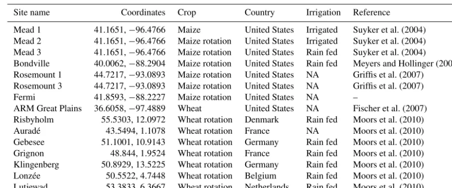
Our analysis focusses on 15 sites for which we can obtain the combination of eddy covariance data, satellite data and crop yield data for specific crops (summarised in Table 1), of which 7 sites were growing maize (Zea mays) and 8 sites were growing winter wheat (Triticum aestivum; we refer to this simply as wheat). Most of these sites grow maize or wheat on a rotation with other crops, and we identify the time period over which the species of interest is growing from the

metadata associated with the eddy covariance data. All of the maize sites are based in the United States. All but one of the wheat sites are based in western Europe, with one site in the United States. For the site where information was available, the crops were not irrigated with the exception of the US-Me1 site (Suyker et al., 2004). All sites have been tilled to a certain degree, generally in accord with agricultural practices in the area. European sites have received a moderate amount of fertiliser (Moors et al., 2010).

2.2 Space-based vegetation indices

We use data on vegetation greenness from the MODIS (Mod-erate Resolution Imaging Spectroradiometer) Terra instru-ment. The MODIS fraction of absorbed photosynthetically active radiation (fAPAR data) from the MOD15A product was downloaded (https://lpdaac.usgs.gov/) for geographic re-gions corresponding to each of the study sites (Table 1) for the period 2000–2010. These data were subsequently filtered using the quality assurance (QA) indices provided so that only data points calculated using the main algorithm were retained and pixels classified as cultivated land were identi-fied using the MODIS land cover product (MOD12A) IGBP classification.

Using the pixel closest to the flux tower site was infea-sible because of data noise and gaps resulting in an uneven time series. Instead, we aggregated all pixels within a 3 by 3 km square centred on the tower site in a single time se-ries. The untested assumption behind this aggregation is that farming practices are constant across this scale. To distin-guish between different crops, we use a crop phenology ap-proach (Wardlow et al., 2007). Pixels that a reach maximum fAPAR before day 150 are classed as winter crops (specifi-cally as winter wheat), while crops that peak after that date are classified as summer crops. This procedure is applied for individual years to account for crop rotations.

2.3 Eddy covariance data

We use eddy covariance data for 15 sites across Europe and the United States (Table 1), consisting of 19 data years. The data were obtained from the AmeriFlux database (http: //ameriflux.lbl.gov/) and the European Fluxes Database Clus-ter (http://www.europe-fluxdata.eu/). We use level-four data of CO2 fluxes partitioned into gross primary productivity

(GPP) and gap filled using the mDS method (Reichstein et al., 2005). Sites that have a crop rotation were filtered to obtain single-species time series. These include the maize– soybean rotation sites and European mix rotation sites that include winter wheat.

2.4 Crop yield data and agricultural dates

(4)

//www.nass.usda.gov/). For the European sites, we used country-level data provided by the EC Eurostat database, available from 2004 onwards (http://ec.europa.eu/eurostat).

Sowing and harvest dates are required as model inputs and were extracted from the crop calendar global dataset (Sacks et al., 2010). We chose this rather than local-level dates for greater model generality.

Fertiliser input data were obtained from the published site descriptions (see Table 1 for references) or from the Nitro-gen Fertilizer Application database (Potter et al., 2010). The model implemented in this study does not require any addi-tional information on irrigation or soil properties.

2.5 Environmental input data

We use NASA’s Modern-Era Retrospective Analysis for Re-search and Application (MERRA) dataset (Rienecker et al., 2011) at a spatial resolution of 0.5◦_{latitude by 0.66}◦ longi-tude and a temporal resolution of 3 h which we average to a day. Temperature as well as direct and diffuse photosyn-thetically active radiation (PAR) data were extracted for each site. Comparison with tower-based meteorological data has shown this to be an accurate estimation of conditions at the tower site for all variables and we use MERRA data for the greater generality of the model as this would allow the model to be applied at any location on the globe.

3 Model description

Our new general model of crop growth is based on the single plant model of Guilbaud et al. (2014) and, like that model, assumes that annual plants show optimal biomass alloca-tion during vegetative growth and optimal flowering in order to achieve maximum reproductive mass given available re-sources. Plant growth is divided into three stages, starting at sowing date and ending at harvest: germination, vegetative growth and reproductive growth.

3.1 Germination

The germination process is described as a degree-day func-tion with a fixed base temperature of 0◦C up to a parame-ter germination limit, germlim. The accumulated degree days,

germacc, are calculated as follows:

germ_acc(t )=

germ_acc(t−1)+(T (t )−Tbase) , T (t )≥Tbase

germ_acc(t−1) , T (t ) < Tbase

. (1)

Vegetative growth begins once the accumulated degree days are higher than the limit parameter, germlim, which is a

free fitted parameter. Initial seed mass is prescribed and is ex-pressed as grams per metre squared, incorporating informa-tion about both seed size and planting density. When the ger-mination limit is reached, all seed mass is allocated to above-ground and belowabove-ground pools according to the optimality

criteria described below. Initial model runs have shown that for values of the germination base temperature T_base and seed mass within realistic ranges, the model is largely insen-sitive to the values of these parameters, which is why they have been fixed.

3.2 Vegetative growth

During vegetative growth, biomass is allocated to either aboveground or belowground fractions to achieve an opti-mal carbon-to-nitrogen (C : N) ratio at the plant level (ρ). The net daily growth is calculated as the minimum of a nitrogen-limited growth rate,Groot, and a carbon-limited growth rate,

Gleaf.

Nitrogen-limited growth is considered to be a function of root massMrootand available soil nitrogenN:

Groot(t )=θ N (t )Mroot(t−1)ρ, (2)

whereθis the nitrogen uptake capacity of the roots expressed as gN g−1soil N g−1root C day−1, N (t ) is soil nitrogen at timet(g) andMroot(t−1)is the root mass (g) at the previous

time step. Carbon-limited growth is considered to be equal to potential net carbon uptake, calculated as the difference between whole canopy photosynthesis and respiration. Pho-tosynthesis is calculated using the model for C3 plants, de-veloped by Farquhar et al. (1980) as described in dePury and Farquhar (1997), and the alternative model for C4 species (Collatz et al., 1992; Von Caemmerer, 2000):

Gleaf(t )=f (Vcmax25, Jm25, T (t ), I (t ), pCO2,

LAI(t−1))−Rplant. (3)

Here,Vcmax25is a parameter representing photosynthetic

Ru-BisCO capacity (µmol m−2s−1), Jm25 is potential electron

transport rate andT,I andpCO2are environmental inputs

(temperature, solar radiation and atmospheric CO2 partial

pressure, respectively). The electron transport rateJm25 is

represented for fitting purposes as the ratiof JbetweenJm25

andVcmax25 to partially eliminate model equifinality. Total

absorbed solar radiationI is calculated for direct and dif-fuse PAR using a sun-shade model (dePury and Farquhar, 1997). Partial pressure of CO2 inside the leaf is calculated

assuming a constant optimal ratioλbetween internal and at-mospheric CO2in the absence of water stress (Haxeltine and

Prentice, 1996) (see Appendix B for details of the photosyn-thesis model in Eq. 3). Leaf area index (LAI) is calculated from leaf mass Mleaf using the leaf mass per area (LMA)

parameter. Whole plant respiration is calculated as a linear function of total plant mass:

Rplant=rtot(Mleaf+Mroot). (4)

Here, rtot represents average respiration per unit plant

(5)

nutrient uptake by the roots and is a function of tempera-ture. Given the optimal whole plant C : N ratio that drives the vegetative biomass allocation, this formulation is ulti-mately equivalent to the nitrogen-dependent function com-monly used in vegetation models without the need to intro-duce further parameters for root- and leaf-specific C : N ra-tios.

Actual biomass growth is then the minimum between nitrogen- and carbon-limited growth:

Gnet=min(Groot, Gleaf). (5)

This biomass is allocated to the limiting fraction, either aboveground or belowground in order to adjust the C : N sup-ply. Crops are considered to be not water limited, as all sites are in areas with high annual precipitation. We lacked any in-formation on soil water availability, and initial trials to data constrain a model that included the effects of varying soil wa-ter availability led to poorly constrained paramewa-ters related to soil water constraints (see Sect. 7).

3.3 Optimal flowering and reproductive growth Reproductive growth starts at a point where the supply of any of the resources, carbon or nitrogen, reaches a maximum, which we term “peak resource”. This is the point in time which will result in the maximum final reproductive mass as further increases in vegetative fractions would not result in an overall increase in growth rate and lead to suboptimal growth (see Guilbaud et al., 2014, for an in-depth discussion of this).

The peak nitrogen condition is achieved when an increase in root mass does not result in an increase in nitrogen up-take. This condition is achieved in nitrogen-limited environ-ments where the nitrogen available in the soil is depleted through the period of vegetative growth. This assumption can be considered valid in agricultural systems where the major nitrogen input into the system during the growing pe-riod comes solely from agricultural fertilisers. Soil nitrogen decays monotonically through the season in our model due to the simplicity with which we model nitrogen uptake, and thus detecting the peak nitrogen condition is straightforward. Similarly, the peak carbon flowering condition is triggered when the addition of aboveground biomass would not lead to an increase in net carbon gain due to self-shading in the canopy. To calculate the peak carbon trigger, we use the en-vironmental variables averaged overpdays, to avoid flower-ing beflower-ing triggered by short-term environmental fluctuations. We inferpalongside the other parameters in our model.

During the reproductive phase, all new biomass produced is assigned to reproductive tissues. Nitrogen and carbon are translocated to reproductive organs at a constant rate,mtrans.

As all biomass within the model is calculated as mass of car-bon, and agricultural yield data are reported as total dry mass, we use a conversion parameter to account for the carbon frac-tion,Cfrac. This parameter also accounts for the differences

in total reproductive mass and actual mass harvested and re-ported as yield.

4 Parameter estimation technique

We use Bayesian parameter inference techniques to infer the parameters for the model described above. The technique in-volves solving Bayes’ theorem which, in this context, states P (θ|obs)=_R P (obs|θ )P (θ )

P (obs|θ )P (θ )dθ, (6)

whereP denotes a probability, obs is the empirical data and θ is the set of parameters to be inferred (Gilks, 1996). The term in the denominator can be treated as a normalising con-stant in our study, and so we omit it here. Thus, our prob-lem reduces toP (θ|obs)≈P (obs|θ )P (θ ), whereP (obs|θ ) is usually referred to as the likelihood of the data given the model andP (θ ) is the prior probability of the parameters. Prior probabilities of parameters can be determined by pre-vious empirical evidence such as field measurements. In our case, we do not have any prior expectations about what the prior parameter values should be and so we specify that each parameter is equally likely to fall within a wide range of val-ues (flat priors). This means that our study reduces to infer-ring the joint probability distribution of the parameters based on the likelihood of the data given all possible parameter combinations. We cannot solve this inference problem ex-actly. Instead, we use Markov chain Monte Carlo techniques with the Metropolis–Hastings algorithm to approximate the likelihood and its associated joint parameter probability dis-tribution, which we implemented using the Filzbach infer-ence library as detailed in Caldararu et al. (2012). This al-gorithm works by iteratively making random mutations to an existing parameter set, computing the likelihood associated with the new set of parameters and then replacing the ex-isting parameter set with the new set based on the ratio of their likelihoods according to the Metropolis–Hastings algo-rithm (Gilks, 1996). Parameter ranges were set based on lit-erature and our understanding of plausible biological ranges for these crop species and agricultural scenarios as well as additional adjustment to ensure parameter convergence dur-ing inference.

(6)

l(Zx|θx)= X

D 1 Nx,D

X

t (x,D)

ln[n(Yobs(x, D, t ), Ypred(x, D, t, θx), σx,D)], (7) whereθx is the vector of model parameters at sitex,Nx is

the number of data points in each datasetDat each location andn(Yobs(x, D, t ), Ypred(x, D, t, θx), σx)denotes the

prob-ability density for observingYobs(x, D, t )given a normal

dis-tribution with meanYpred(x, D, t, θx)and standard deviation

σx,D which expresses the magnitude of unexplained varia-tion in the variableY.Y refers to the model variables corre-sponding to the three datasets. Note that with this definition of the likelihood we are treating every data point as inde-pendent; that is, the likelihood of a value at timet is treated independently from the likelihoods at preceding times. This is only an approximation but is commonly used in param-eter estimation studies because the additional mathemati-cal and computational complexity of accounting for non-independent data.

We adopt different techniques to estimate the standard de-viationσx,Dabove, depending on the datasetD at each lo-cation. Generally, we assume that the variation in the model predictions about the data is solely due to uncertainty in the data. We address the limitations of this assumption and fu-ture improvements in the Discussion section. The GPP data do not have an estimate of uncertainty, and so we infer the un-certainty associated with those data as the parameterσx,D. In the case of MODIS fAPAR data, we explicitly incorporate a measure of variation in the data within the geographical area used to compute the mean fAPAR while inferring a parame-ter representing additional unexplained variation. We include this parameter to account for known issues in space-based re-motely sensed data, such as background soil reflectance. The crop yield data already have estimates of observational un-certainty associated with them, and so we use those data to defineσx,D.

5 Experimental protocol

In order to assess whether the model with data-constrained parameters predicts empirical data better than a model with prior parameters, we infer the parameters for each site in-dividually using all of the empirical data and compare the model predictive performance to one site in which the pa-rameter values are sampled randomly from the prior range.

We compare the inferred parameters and predictive perfor-mance of models with parameters inferred using data from individual sites (the one-site model) or from multiple sites together (all-site model), always keeping maize and winter wheat sites separate, to assess the effects of allowing param-eters to differ between the sites. Preliminary investigations revealed that similar model parameter distributions were

in-ferred once data from more than three sites were used in com-bination when inferring the parameters. We therefore also take the opportunity to assess the performance of the mod-els with parameters shared between sites in predicting data that have not been used in parameter inference (evaluation model).

To assess the importance of different types of data con-straints, we perform a data knock-out experiment and we in-fer the model parameters for individual sites using only one or two of the different empirical datasets and assess inferred model parameters and model performance.

In general, we assess model predictive performance by quantifying the root mean squared error (RMSE) between the model predictions and the empirical data to access model precision and the mean error to assess model bias. We nor-malise both these metrics by the mean value of the different empirical dataset types to aid in comparison. We calculate parameter uncertainty as the 95th percentile confidence in-terval from the posterior distribution (Sect. 4).

To calculate uncertainty for the model predictions, we sample parameter values from their respective posterior dis-tribution and compute predictions with each parameter com-bination, which results in a corresponding distribution of model predictions. We report this prediction distribution un-certainty using 95th percentile confidence intervals. This pre-dicted distribution does not include the prescribed or inferred uncertainty about observations,σx,D; our predicted distribu-tions correspond to the state being predicted and not the ob-servations of that state.

6 Results

6.1 Prior and posterior model predictions

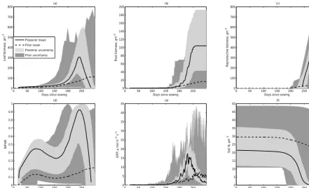
In general, and as expected, the predictive accuracy of both the wheat and maize models is improved by inferring their parameters; the root mean squared error and bias of the model predictions is reduced for predicting all empirical datasets compared to the prior model (Table 3). These im-provements are about a 40 % reduction in RMSE for both GPP and fAPAR and an 80 % reduction in RMSE for yield. Visual inspection of the predicted time series for the models with prior and posterior parameter distributions (e.g. Fig. 1 for wheat in one site) highlights that the model with prior parameters predicts the same qualitative behaviour as the model with inferred parameters but that parameter inference reduces the posterior uncertainty in the predictions of the model.

(7)

0 50 100 150 200 250 0 100 200 300 400 500 600 700 800

Days since sowing

Leaf biomass, gm

−2 (a) Posterior mean Prior mean Posterior uncertainty Prior uncertainty

0 50 100 150 200 250 0 20 40 60 80 100 120 140 160 180 200

Root biomass, gm

−2

Days since sowing (b)

0 50 100 150 200 250 0 100 200 300 400 500 600 700 800

Reproductive biomass, gm

−2

Days since sowing (c)

0 50 100 150 200 250 0 0.1 0.2 0.3 0.4 0.5 0.6 0.7 0.8 0.9 1 fAPAR

Days since sowing (d)

0 50 100 150 200 250 0 5 10 15 20 25 30 35 40 45 GPP, mol m −2 s −1

Days since sowing (e)

0 50 100 150 200 250 0 5 10 15 20 25 30 35 40 45 50

Soil N, gm

−2

Days since sowing (f)

Figure 1.Comparison of prior model predictions (dark grey, dashed line) and posterior model predictions (light grey, continuous line) at one wheat (DK-Ris) site. Panels show(a)aboveground biomass,(b)belowground biomass,(c)reproductive biomass,(d)fAPAR,(e)GPP and

(f)soil nitrogen.

emphasises the importance of model structural constraints on the model dynamics; e.g. the model predicts a narrow range of dynamics in some properties at certain times of the year (e.g. biomass in leaves, roots and reproductive parts soon af-ter sowing) irrespective of the parameaf-ter values.

6.2 One site’s versus all sites’ fit

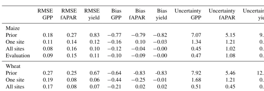
On average, the RMSEs are very similar between the models with parameters inferred for individual sites to when param-eters are inferred for all sites together (Table 3). In general, we expect that if we were to infer a single set of parame-ters for individual sites, then the predictive performance of that model will always be at least as good as when the set of parameters has been inferred for all sites. This may not nec-essarily be the case when inferring parameter probability dis-tributions: the lower quantity of data could result in greater parameter uncertainty which may on average lead to a lower predictive accuracy than that using the more constrained pa-rameter distributions obtained by inferring papa-rameters from all sites. This explains why some of the mean RMSE scores are higher for the model with parameters inferred from indi-vidual sites. The bias scores are also very similar, although the bias tends to be smaller on average for the models with parameters inferred using all sites.

As expected, the uncertainty in the predicted GPP, fAPAR and yield is lower for the models with parameters inferred us-ing all sites because more data are used to infer the parameter values for those models, leading to lower uncertainty in the inferred parameter distributions (Fig. 2). When parameters are inferred for individual sites, uncertainty is around 134 % for GPP, 121 % for fAPAR and 33 % for yield, with simi-lar values at wheat sites (Table 3). This is reduced to around 45 % for GPP, 100 % for fAPAR and 12 % for yield estimates when parameters are inferred using data for all sites. Visual inspection of the change in uncertainty over time highlights that prediction uncertainty due to parameter uncertainty is highest at the start and end of the season (over 100 %) but decreases to 50 % on average for all variables in the middle of the growing period (Fig. 4).

(8)

veg-Table 1.Study sites are listed; all sites correspond to eddy covariance measurement sites.

Site name Coordinates Crop Country Irrigation Reference

Mead 1 41.1651,−96.4766 Maize United States Irrigated Suyker et al. (2004)

Mead 2 41.1651,−96.4766 Maize rotation United States Irrigated Suyker et al. (2004) Mead 3 41.1651,−96.4766 Maize rotation United States Rain fed Suyker et al. (2004) Bondville 40.0062,−88.2904 Maize rotation United States Rain fed Meyers and Hollinger (2004) Rosemount 1 44.7217,−93.0893 Maize rotation United States NA Griffis et al. (2007)

Rosemount 3 44.7217,−93.0893 Maize rotation United States NA Griffis et al. (2007)

Fermi 41.8593,−88.2227 Maize rotation United States NA –

ARM Great Plains 36.6058,−97.4889 Wheat United States NA Fischer et al. (2007)

Risbyholm 55.5303, 12.0972 Wheat rotation Denmark Rain fed Moors et al. (2010)

Auradé 43.5494, 1.1078 Wheat rotation France NA Moors et al. (2010)

Gebesee 51.1001, 10.9143 Wheat rotation Germany Rain fed Moors et al. (2010)

Grignon 48.844, 1.9524 Wheat rotation France Rain fed Moors et al. (2010)

Klingenberg 50.8929, 13.5225 Wheat rotation Germany Rain fed Moors et al. (2010)

Lonzée 50.5522, 4.7448 Wheat rotation Belgium Rain fed Moors et al. (2010)

Lutjewad 53.3833, 6.3667 Wheat rotation Netherlands Rain fed Moors et al. (2010)

NA=not available

Maize Wheat 50 100 150 200 250 300 350 400 Vcmax25 ,

mol C m

-2 s -1 Maize Wheat 2 3 4 5 6 7 8 9 10 fJ, Maize Wheat 100 150 200 250 300 350 400

LMA,g C m

-2 Maize Wheat 1 2 3 4 5 6 7 8 9 10

,g N g

-1 N g -1 C day -1 Maize Wheat 0.05 0.1 0.15 0.2 0.25 0.3 rtot ,g g -1 Maize Wheat 2 4 6 8 10 12 14 16 18 20 trans,g Maize Wheat 100 150 200 250 300 350 400 germ lim ,

° C

Maize Wheat 10 20 30 40 50 60 70 80 90 100 N0 ,g m -2 Maize Wheat 0.2 0.3 0.4 0.5 0.6 0.7 0.8 0.9 1 Cfrac , Maize Wheat 0.1 0.2 0.3 0.4 0.5 0.6 0.7 0.8 0.9 0 , Single site All sites

(9)

Table 2.Model parameters, upper and lower bounds and initial values used in the model-fitting procedure.

Symbol Units Description Lower bound Upper bound Initial value Fixed

germ_lim ◦C Number of degree days required 100.0 400.0 150.0 no

for germination

Tb_germ ◦C Base temperature for germination – – 0.0 yes

ρ – Optimal carbon-to-nitrogen ratio in – – 25.0 yes

vegetative tissue

N₀ g Initial N content of the soil 10.0 100.0 15.0 no

θ g N g−1N g−1C day−1 Root nitrogen extraction factor 0.0005 0.01 0.0005 no

V_cmax25 µmol m−2s−1 Photosynthetic carboxylation capacity at 25◦C 50.0 400.0 80.0 no

f J – Ratio of electron transport to 2.0 10.0 2.1 no

carboxylation capacity at 25◦C

λ₀ – Ratio of atmospheric and leaf CO₂ 50.0 400.0 80.0 no

concentration

LMA g m−2 Leaf mass per area 60.0 400.0 100.0 no

rtot g g−1 Average plant respiration rate 0.001 0.3 0.1 no

mtrans g day−1 Mass translocation rate from vegetative 0.1 20.0 2.0 no

to reproductive tissue

C_frac – Carbon fraction of reproductive tissue 0.2 1.0 0.7 no

p days Time period for averaging environmental 1.0 30.0 10.0 no

conditions for flowering trigger

Table 3.Model RMSE, bias and uncertainty for the one-site and all-site parametrisation as well as the model evaluation run.

RMSE RMSE RMSE Bias Bias Bias Uncertainty Uncertainty Uncertainty

GPP fAPAR yield GPP fAPAR yield GPP fAPAR yield

Maize

Prior 0.18 0.27 0.83 −0.77 −0.79 −0.82 7.07 5.15 9.87

One site 0.11 0.14 0.12 −0.16 0.10 −0.03 1.34 1.21 0.33

All sites 0.08 0.16 0.10 −0.12 −0.04 −0.00 0.45 1.02 0.12

Evaluation 0.09 0.15 0.11 −0.10 −0.09 −0.00 0.47 1.08 0.15

Wheat

Prior 0.27 0.25 0.67 −0.64 -0.83 -0.83 7.92 5.46 12.27

One site 0.19 0.08 0.06 −0.44 −0.25 −0.01 1.68 1.21 0.16

All sites 0.17 0.08 0.07 −0.21 0.02 0.02 0.51 0.45 0.06

Evaluation 0.17 0.09 0.07 −0.05 −0.26 0.02 0.75 0.89 0.08

etative to reproductive tissue. These inferred differences are probably due to differences in winter wheat crops between the US site and the European sites, such as different crop va-rieties or agronomic practices.

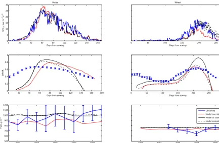
Visual inspection of the predicted time series of GPP, fA-PAR and yield for maize and winter wheat predominantly show very similar predictions between the models with pa-rameters estimated from one site versus all sites (Fig. 3 shows predictions for representative sites; Appendix A shows time series for all sites with associated uncertainty). There tends to be greater differences between the model predictions and the empirical data when the model has site-specific parametrisa-tions than when parametrisaparametrisa-tions are shared between sites. The one notable exception is again the winter wheat site in the US, for which inferring parameters for the specific site

(10)

0 20 40 60 80 100 120 140 160 0

5 10 15 20 25 30

GPP,

mol m

−2

s

−1

Maize

Days from sowing

0 20 40 60 80 100 120 140 160 180 0

0.2 0.4 0.6 0.8 1

fAPAR

Days from sowing

2001 2003 2005 2007 2009

500 600 700 800 900 1000 1100 1200

Yield, g m

−2

Year

0 50 100 150 200 250

Wheat

Days from sowing

0 50 100 150 200 250 300

Days from sowing

2001 2003 2005 2007 2009

Year

Observed Model one site Model all sites Model evaluation

Figure 3.GPP, fAPAR and yield model predictions at one maize site (US-Ro3) and one wheat site (DE-Gri). The figure shows posterior mean predictions for one site, all sites and the evaluation model fit. Neither site has been included in the evaluation fitting.

we attribute this at least in part to the data themselves having a relatively high uncertainty (discussed further below).

We evaluate the model transferability by inferring the model parameters using a subset of the sites and assess-ing model predictive performance against the remainassess-ing sites (Fig. 3 and Table 3). In general, the model RMSE and bias do not differ between the sites that were used for parame-ter estimation and those that were not. Moreover, the model predictive performance is similar to that resulting when fit-ting to all sites. The uncertainty for GPP, fAPAR and yield at maize sites is similar to that obtained by fitting to all sites, but for the wheat sites the uncertainty in GPP and fAPAR increases, while the yield uncertainty remains at the level ob-tained when fitting to all sites (Table 3).

6.3 Impacts of using different data types

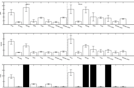
Our data-type hold-out experiments show clear differences in the roles played by different data types in improving model predictive accuracy, but the effects are similar for both crop types (Fig. 5 – this figure only shows model RMSE and bias when parameters are inferred using data for individual sites, but the results are similar when all sites are used to infer model parameters). The largest effect of adding a given data type is when yield data are included, which significantly re-duces RMSE and bias for predicting yield. This makes intu-itive sense, although interestingly including yield data alone

and as part of a combination also tends to improve model pre-dictive performance for GPP and fAPAR. Counterintuitively, including GPP data alone or fAPAR data alone only has sub-tle effects on the model RMSE and bias for predicting those variables and yield, but including those datasets in combina-tion does indeed lead to improvements in RMSE and bias.

The greatest improvements in model predictive perfor-mance for all response variables is obtained when all data types are used for parameter inference. This is not inevitable as an overall more likely model might be achieved by sacri-ficing predictive accuracy for one data type in order to im-prove predictive accuracy for another. For example, adding fAPAR data alone slightly improves model RMSE for fA-PAR data, but makes it worse for GPP and yield predic-tions when compared to the model with prior parameter distributions. Indeed, the crops do not flower for maize or wheat when only fAPAR data are used for parameter infer-ence. Comparing knockouts with and without fAPAR data included implies a trade-off between predicting the fAPAR data well and predicting GPP well (Fig. 5). Interestingly, all models underestimate GPP, although this bias is least when all data are used to infer the model parameters.

(11)

0 0.5 1 1.5 2 2.5 3 3.5

GPP

mol m

−2 s

−1

Maize Wheat

0 0.5 1 1.5 2 2.5 3 3.5

fAPAR

70 80 90 100 110 120 130 140 150 160 170 0

0.5 1 1.5 2 2.5 3 3.5

Reproductive biomass, gm

−2

Days from sowing

190 200 210 220 230 240 250 260 270 280 Days from sowing

Model one site Model all sites Model evaluation Model one site Model all sites Model evaluation

Figure 4.Normalised uncertainty for GPP, fAPAR and yield model predictions at one maize site (US-Ro3) and one wheat site (DE-Gri). Uncertainty is calculated as 95th percentile confidence bounds normalised by the posterior mean for one site, all sites and the evaluation model fit. Neither site has been included in the evaluation fitting.

Table 4.RMSE, bias and uncertainty values in the data knock-out experiments for wheat and maize.

Data RMSE RMSE RMSE Bias Bias Bias Uncertainty Uncertainty Uncertainty

fitted to GPP fAPAR yield GPP fAPAR yield GPP fAPAR yield

Maize

Prior 0.18 0.26 0.85 −0.75 −0.79 −0.85 6.91 5.19 9.25

All data 0.11 0.14 0.12 −0.16 0.10 −0.03 1.34 1.21 0.33

fAPAR 0.31 0.21 1.00 −0.90 −0.86 −1.00 8.99 3.53 –

GPP 0.12 0.20 0.80 −0.28 0.20 −0.79 1.66 1.24 2.83

Yield 0.17 0.17 0.12 −0.48 0.30 −0.05 3.61 1.42 0.33

GPP+yield 0.12 0.18 0.79 −0.30 0.08 −0.78 1.58 1.26 2.72

fAPAR+yield 0.11 0.15 0.11 −0.17 0.07 −0.03 1.23 1.28 0.31

fAPAR+GPP 0.18 0.15 0.11 −0.50 0.07 −0.04 3.69 1.57 0.32

Wheat

Prior 0.28 0.25 0.70 −0.66 −0.84 −0.88 8.49 5.90 12.98

All data 0.19 0.08 0.06 −0.44 −0.25 −0.01 1.68 1.21 0.16

fAPAR 0.37 0.19 0.80 −0.92 −0.82 −1.00 8.02 3.59 –

GPP 0.32 0.12 0.73 −0.81 −0.48 −0.92 4.04 2.21 –

Yield 0.28 0.08 0.06 −0.60 −0.23 −0.01 3.55 1.67 0.16

GPP+yield 0.28 0.11 0.69 −0.73 −0.40 −0.86 3.38 1.94 –

fAPAR+yield 0.21 0.09 0.06 −0.50 −0.28 −0.02 1.63 1.21 0.16

(12)

0 0.1 0.2 0.3 0.4 0.5

Maize Wheat

RMSE

GPP

Prior All datafAPARGPP Yield GPP+yieldfAPAR+yieldfAPAR+GPPPrior All datafAPARGPP Yield GPP+yieldfAPAR+yieldfAPAR+GPP

0 0.1 0.2 0.3 0.4

fAPAR

0 0.5 1 1.5

Yield

Prior All datafAPARGPP Yield GPP+yieldfAPAR+yieldfAPAR+GPPPrior All datafAPARGPP Yield GPP+yieldfAPAR+yieldfAPAR+GPP −1 −0.5 0 0.5

Maize Wheat

Residuals

−1 −0.5 0 0.5 1

−1 −0.5 0 0.5

Figure 5.Model RMSE and bias for all data hold-out experiments averaged over all wheat and maize sites, respectively. Error bars represent variation across sites. All values have been normalised to the mean value of that variable at each site. Black bars indicate models that do not reach flowering.

values of 123, 128 and 32 % for GPP, fAPAR and yield, re-spectively – values which are close to those obtained through fitting to all the data. The GPP and yield model also has rel-atively low uncertainty values for GPP and fAPAR estimates but fails to produce any yield at the wheat sites (the plants do not proceed to the flowering stage).

7 Discussion

7.1 Model performance

We show that a process-based crop model (PeakN-crop v1.0) constrained using EC data, satellite fAPAR observations and regional yield estimates can improve model performance compared to the model run with prior parameter ranges and greatly reduces the uncertainty in model output. However, the resulting uncertainty in both state variables and model parameters is still relatively high.

Model uncertainty is difficult to compare with previous crop modelling studies, as models with fixed parameter val-ues do not often provide uncertainty estimates. In fact, pro-viding uncertainty values for all model variables and

param-eters is one of the advantages of a data-constrained model. In the current model, uncertainty is highest at the start of the season for all variables but decreases rapidly and final yield uncertainty is much lower. This is due to thresholds: abrupt changes from one growing stage to another when small dif-ferences in parameters can lead to large difdif-ferences in result-ing variables. It is, however, important to note that the uncer-tainty in our yield predictions remains high and the model in its current form is unlikely to provide accurate predic-tions for practical applicapredic-tions without the addition of new data (Sect. 7.4). We have, however, shown that the use of three different data types does reduce prediction uncertainty – pointing to an avenue for future model improvement.

(13)

0 2 4 6 8 10 12

Maize Wheat

GPP

Prior All data fAPAR GPP Yield GPP+yield fAPAR+yield fAPAR+GPP Prior All data fAPAR GPP Yield GPP+yield fAPAR+yield fAPAR+GPP

0 2 4 6 8

fAPAR

0 5 10 15 20

Yield

Figure 6.Model uncertainty, expressed as the difference between the upper and lower 95th confidence intervals for all model setups averaged across all wheat and maize sites. Error bars represent variation between sites. All values have been normalised. Black bars indicate models that do not reach flowering.

made if our model is applied to real agricultural prediction scenarios.

In terms of the posterior parameter distributions, result-ing parameters show a similar degree of constraint to that observed in previous model parametrisation studies for nat-ural ecosystems (Keenan et al., 2012). The photosynthesis-related parameters are badly constrained despite the fact that GPP estimates have a relatively low uncertainty. This can be explained by the structure of the photosynthesis component which is rigid compared to other components of the model as these processes are better understood. In contrast, below-ground processes are both poorly understood and lack the data to properly constrain model parameters (Pendall et al., 2004).

In terms of model performance, the model correctly pre-dicts seasonal trajectories of GPP and final yield data. We cannot, however, capture the interannual variability in yields, which is most likely due to the fact that our model does not include a response to water limitation or heat damage. The fact that we use regional yield data can also lead to discrep-ancies between the yield at each specific flux tower site and the yield data. The model does not capture the fAPAR sea-sonal cycle well, especially at the maize sites, which is due to the low spatial resolution of the data. However, the predicted model fAPAR is more realistic than the fAPAR data, which

is one of the advantages of using a process-based model with a more rigid structure than a statistical one.

One additional complication is the different spatial scales of the three datasets; while the eddy covariance data are at the scale of the flux tower footprint, which can be seen as equivalent to the individual field scale, the fAPAR and yield data correspond to larger scales (county and country level for the yield data and a 3 by 3 km scale for the fAPAR data). The assumption behind our analysis is that the conditions at field scale are representative of the regional scale, so that there would be no discrepancy between model predictions at these different scales. This is obviously a source of error, especially at the wheat sites in Europe, which will be located over a much more heterogeneous landscape. Further sources of data at the field scale would be required to identify the model error caused by the discrepancy in spatial scales.

7.2 Use of the different datasets

(14)

this fact is maybe not surprising. The seasonality information is already contained in the fAPAR dataset, while the primary productivity is highly constrained by the structure of the bio-chemical photosynthesis model. Furthermore, the GPP-only fit results in an underestimation of the final yield, indicating that the sole use of EC data in crop models is not sufficient to accurately predict yields. Unlike most studies using EC data, we have used sites with only 1 year of data as these were the only available agricultural sites, and it is possible that more GPP data at one site could increase its importance in the fit-ting. EC data could also be a valuable tool for independent model evaluation, as they provides information about plant function not included in the other available data.

Space-based vegetation data have the main advantage of a large spatial and temporal coverage, so that they can be used irrespective of the local monitoring infrastructure, providing a general data source. However, the quality of the data is rel-atively low, especially at the high spatial resolutions needed for crop modelling. This problem is particularly obvious in the case of the maize data, which lack the expected seasonal-ity and are reflected in the very high error in the fAPAR-only fit. However, the model fits without fAPAR (GPP and yield only) show a high error as well, indicating that the informa-tion content in vegetainforma-tion indices is needed for constraining the model but is not sufficient.

Some of these limitations are not general for remotely sensed data but can be attributed to the spatial and spectral resolution of the MODIS instrument. The 1 km spatial res-olution can be too coarse for agricultural fields, especially in areas with heterogeneous land cover. Other existing in-struments, specifically the Landsat family, have a better spa-tial resolution (30 m), but a much poorer temporal resolution which we have found unsuitable for fitting a plant growth model where developmental changes can be abrupt. More re-cent missions such as Sentinel-2 will have more suitable spa-tial and temporal resolutions for use with this type of model (Herrmann et al., 2011). Some of the errors in the data can also be attributed to misclassification of pixels. We use a sim-ple phenology-based approach which is one of the only ones available for data with a relatively wide bandwidth, such as MODIS. This method is useful for winter crops which have different timing compared to the natural vegetation, but less useful for summer crops such as maize where there is no clear separation in phenology between cropland and the sur-rounding vegetation. Hyperspectral data can be used more accurately for crop identification (Thenkabail, 2001) but to date no space-based instrument is available that has the re-quired bandwidth, the spatial and temporal coverage and the spatial and temporal resolution. However, such data should be used at local scales if the measurements are available.

Crop yield is the data that are traditionally used for evalu-ating agricultural models and is arguably the most important to predict correctly, given that the purpose of the model is to predict crop productivity. We have used county- and country-level reported yields rather than field-country-level measured yield

because of both the availability of the data and the generality of the method. The model fitted with yield data only gives a good fit to yields but gives higher errors for the GPP and fA-PAR estimates, which raises questions about the correctness of models which only use final yields to assess performance and the ability of such models to predict crop yields under different conditions. Crop yield data provide the final point of plant crop growth but there is potentially a multitude of model structures and parameter combinations that can result in that yield.

In addition to the three datasets used for parametrisation, the model also requires input data in the form of sowing and harvest dates and fertiliser inputs. Additional uncertainty is associated with these datasets which is not available nor ac-counted for in our analyses. For example, the crop calendar (Sacks et al., 2010) and Nitrogen Fertilizer Application (Pot-ter et al., 2010) datasets are global data collections that will imperfectly represent the value for any given location. Al-ternatives to these global datasets would be to use location-specific data or to infer the values. Location-location-specific data have the advantage of more accurately reflecting the situa-tion at a given site and would therefore be useful when the model is applied at the field scale, but such data are unlikely to be available for all sites. Successful inference of the val-ues would depend on if there is enough information in the datasets used to infer the model parameters. If there are in-adequate data, then there would be excessive degrees of free-dom for inference, leading to the wrong parameter values be-ing inferred and the model performbe-ing poorly in novel situa-tions. Therefore, the decision whether to obtain more data or infer unknown quantities in future applications of our model and inference framework depends on the data availability and the intended scales of application.

7.3 Choice of model

(15)

7.4 Future data needs

The fact that our model shows a relatively good fit when con-strained at multiple sites indicates that it would be possible to obtain a single parameter set for one cultivar given the same agricultural practices, so that the model can be fitted at a small number of locations and then applied more widely. However, the parameters are badly constrained and part of the data we have used are not sufficiently accurate to allow the use of the model at a wider variety of locations and cli-mate conditions. Accurate yield data are essential but not suf-ficient and must be accompanied by a growth time series. Our results indicate that additional EC data are not necessary, es-pecially given the cost of installing and maintaining a flux tower. Instead, either biomass or LAI (or fAPAR or other vegetation indices) data could be easier to obtain at multi-ple locations. The belowground part of the model, describing root nitrogen uptake, is only indirectly constrained by the ex-isting data, and any observation of root mass and function would have the capacity to add extra information, especially time series information (Johnson et al., 2001).

The model in the version presented in this paper does not include any water limitation to growth due mainly to a lack of data constraint on any water-related parameters, as we found that latent heat data from EC towers are not sufficient. Below-ground measurements of not only root growth but also soil water properties would again provide some of the necessary information. Such belowground data, especially if supple-mented by nutrient concentrations, can also help constrain a more complex version of the nitrogen uptake scheme, which could be improved to include more explicit soil–plant inter-actions and additional processes such as biological nitrogen fixation for legumes.

If this model, or any other similar process-based data-constrained crop model, is to be used for scientific purposes to understand the response of crops to climate across the globe, the ideal data would be a global dataset, such as space-based vegetation observations, combined with high-quality field-level data that would ideally include growth time series, final grain yield and information about agricultural practices. However, if the model is to be used for agricultural purposes, to aid decision making at the local level, high-quality field-level data would be sufficient. A valuable evaluation in such studies, not conducted here for brevity and due to a lack of location-specific data, would be to compare the predictive ac-curacy of the model against the predictive acac-curacy of a sta-tistical average over the data. Such an analysis would reveal whether and how much benefit is gained by using a data-constrained model for predictions.

8 Conclusions

In this paper, we present a method for data constraining a process-based agricultural model to three sources of data: eddy covariance flux measurements, space-based fAPAR and regional yield estimates. We show that the data-constrained model performs better than the model with prior parameter estimates, especially in terms of uncertainty, and even though the data used are in some cases not sufficient to fully con-strain posterior parameters, they have sufficient information values to be used for model parametrisation. We apply the model to both maize and wheat sites and show that the model performs equally well for both species. Parameters can be shared between sites of the same species with a similar per-formance to local parameters and reduced uncertainty. We have also investigated the impact of the different datasets on constraining the model, and we show that all three types of data contribute to the model performance, but that if in a data-limited world one of the data types was not available, the model can be constrained reasonably well with fAPAR and yield data only. There are still gaps in the data avail-able for model parametrisation, which are also a limitation to the models that can be parametrised, in particular in rela-tion to water limitarela-tion on crops, and we believe that a model parametrisation framework such as that presented here can help identify those gaps and the data needed to further our capacity to model crops.

Code and data availability. All model code used in this paper is available from the authors upon request.

(16)

Appendix A: Site-level model simulations

(17)

0 10 20 30 40 50

US−Ne1 US−Ne2 US−Ne3 US−Bo1 US−Ro1

0 10 20 30 40 50

US−Ro3

GPP,

mol m

−2

s

−1

US−IB1 US−ARM DK−Ris FR−Aur

0 100 200 300 400 0

10 20 30 40 50

DE−Geb

0 100 200 300 FR−Gri

0 100 200 300 400 DE−Kli

Days from sowing

0 100 200 300 BE−Lon

0 100 200 300 400 NE−Lut

Model one site Model all sites Flux GPP

Figure A1.Gross primary production predictions for 1 year for all sites fitted using all available data at each individual site and at all sites together. Grey shaded areas represent 95 % confidence intervals drawn from the posterior distribution.

0 0.2 0.4 0.6 0.8

US−Ro3

fPAR

0 100 200 300 0

0.2 0.4 0.6 0.8

DE−Geb

0 100 200 FR−Gri

0 100 200 300 DE−Kli

Days from sowing

0 100 200 BE−Lon

0 100 200 300

NE−Lut Model one site Model all sites MODIS

(18)

500 1000 1500 2000

US−Ro3

Yield, g m

−2

2001 2003 2005 2007 2009 500

1000 1500 2000

DE−Geb

2001 2003 2005 2007 2009 FR−Gri

2001 2003 2005 2007 2009 DE−Kli

Years

2001 2003 2005 2007 2009 BE−Lon

2001 2003 2005 2007 2009 NE−Lut

Model one site Model all sites Measured

Figure A3.Yield predictions for all years for all sites fitted using all available data at each individual site and at all sites together. Grey shaded areas represent 95 % confidence intervals drawn from the posterior distribution.

0 5 10 15 20 25

US−Ro3

GPP,

mol m

−2 s

−1

0 100 200 300 400 0

5 10 15 20 25

DE−Geb

0 100 200 300 FR−Gri

0 100 200 300 400 DE−Kli

Days from sowing

0 100 200 300 BE−Lon

0 100 200 300 400 NE−Lut

Model all sites Flux GPP

(19)

0 0.2 0.4 0.6 0.8

US−Ro3

fPAR

0 100 200 300 0

0.2 0.4 0.6 0.8

DE−Geb

0 100 200

FR−Gri

0 100 200 300 DE−Kli

Days from sowing

0 100 200

BE−Lon

0 100 200 300 NE−Lut

Figure A5.fAPAR predictions for 1 year for all sites fitted using all available data at a subset of sites for model evaluation. Sites with black boxes have been used in the model fitting. Grey shaded areas represent 95 % confidence intervals drawn from the posterior distribution.

200 400 600 800 1000 1200

GPP,

mol m

−2

s

−1

200 400 600 800 1000 1200

US−Ro3

Yield, g m

−2

US−IB1

Days from sowing

US−ARM DK−Ris FR−Aur

20012003200520072009 200

400 600 800 1000 1200

DE−Geb

20012003200520072009 FR−Gri

20012003200520072009 DE−Kli

Years

20012003200520072009 BE−Lon

20012003200520072009 NE−Lut

Measured Model all sites

(20)

Appendix B: Photosynthesis model

In the current study, we use the standard biochemical model of Farquhar et al. (1980) for C3 photosynthesis, using the pa-rameter values from dePury and Farquhar (1997). The model stipulates that the photosynthesis rate is defined as the mini-mum of two rates, RuBisCO-limited photosynthesis,Av, and electron-transport-limited photosynthesis:

A=min(Av, Aj). (B1)

RuBisCO-limited photosynthesis is a function of the

param-eterVcmax25, adjusted for temperature, and the internal CO2

partial pressure,ci: Av=Vcmax

ci−0∗ ci+K0

. (B2)

Here,Vcmaxis the adjusted for temperature value ofVcmax25

using the Arrhenius function (see Table B1 for defini-tions and values of photosynthetic parameters). The electron transport-limited rate is calculated as

Ak=J

ci−0∗ 4(ci+20∗)

, (B3)

whereJis the solution to the quadratic equation of

2J2−(Ia+Jm)J+IaJm=0. (B4)

Here,Jmis the temperature-adjusted value of the model

pa-rameterJm25, andIa is the PAR absorbed by the

photosys-tem: Ia=I

(1−f )

2 . (B5)

The parametersVcmax25andJm25are free parameters in the

model (Table 2) and are the values of carboxylation capacity and electron transport at a temperature of 25◦C, whileVcmax

andJn are the parameters at the current temperature, calcu-lated using the Arrhenius function.

Table B1.Photosynthesis model constants according to dePury and Farquhar (1997) for C3 photosynthesis and adapted from Haxeltine et al. (1996) for C4 photosynthesis.

Symbol Units Description C3 value C4 value

0∗ Pa CO2compensation point 3.69 0

K0 Pa Effective Michaelis–Menten constant of RuBisCO 73.8 94.61

2 – Curvature of leaf response of electron transport to irradiance 0.7 0.7

f – Spectral correction factor 0.15 0.15

The internal CO2 partial pressure is calculated based on

the assumption that plants maintain a constant ratio between atmospheric and internal partial pressure in the absence of water stress:

λ=ci

ca

, (B6)

whereca is the atmospheric CO2 partial pressure and is a

model input andλis a free model parameter.

In the case of C4 photosynthesis, the standard biochemi-cal model includes a third limitation, the PEP-carboxylation rate (Collatz et al., 1992; Von Caemmerer, 2000), and we have used a simplification of this model, adapted from Hax-eltine et al. (1996) which uses different biochemical con-stants to reach an equivalent photosynthesis rate using only the RuBisCO- and electron transport-limited rates, which is independent of CO2and temperature in non-extreme

condi-tions.

We calculate the PAR absorbed by the canopy as a sum of absorbed direct and diffuse radiation:

I=Idirect0(1−ekdirectLAI)+Idiffuse0(1−ekdiffuseLAI), (B7)

wherekdirect andkdiffuse are light extinction coefficients for

the direct and diffuse components of radiation, respectively,

andIdirect0andIdiffuse0are the two respective components of

PAR at the top of the canopy and are environmental drivers for the model. The diffuse radiation coefficient is assumed to be a constant and set to 0.7 (unitless) while the direct ex-tinction coefficient varies with the day of year and latitude as follows:

kdirect=

0.5

sinβ, (B8)

whereβis the sun elevation angle:

sinβ=sin3sinδ+cos3cosδ. (B9)

Here,3is the site latitude andδis the sun declination angle calculated at noon, given the model time step of 1 day, as a function of the day of the year (DOY):

δ=23.45 sin

2πDOY+284 365

(21)

Author contributions. All authors contributed to model develop-ment and analysis.

Competing interests. The authors declare that they have no conflict of interest.

Acknowledgements. We would like to acknowledge all data providers for the eddy covariance flux site data. Funding for AmeriFlux data resources was provided by the US Department of Energy’s Office of Science. We would also like to thank the developers of the MODIS fAPAR product used in this study. We thank Christoph Müller, Daniel Wallach and an anonymous reviewer for their constructive comments that greatly improved our manuscript.

Edited by: C. Müller

Reviewed by: D. Wallach and one anonymous referee

References

Baldocchi, D. D. and Wilson, K. B.: Modeling CO2 and

wa-ter vapor exchange of a temperate broadleaved forest across hourly to decadal time scales, Ecol. Model., 142, 155–184, doi:10.1016/S0304-3800(01)00287-3, 2001.

Bondeau, A., Smith, P. C., Zaehle, S., Schaphoff, S., Lucht, W., Cramer, W., Gerten, D., Lotze-campen, H., Müller, C., Reich-stein, M., and Smith, B.: Modelling the role of agriculture for the 20th century global terrestrial carbon balance, Glob. Change Biol., 13, 679–706, 2007.

Brisson, N., Gary, C., Justes, E., Roche, R., Mary, B., Ripoche, D., Zimmer, D., Sierra, J., Bertuzzi, P., Burger, P., Bussière, F., Cabidoche, Y. M., Cellier, P., Debaeke, J. P., Gaudillère, P., Hé-nault, P., and Maraux, F.: An overview of the crop model STICS, Eur. J. Agron., 18, 309–332, 2003.

Caldararu, S., Palmer, P. I., and Purves, D. W.: Inferring Ama-zon leaf demography from satellite observations of leaf area index, Biogeosciences, 9, 1389–1404, doi:10.5194/bg-9-1389-2012, 2012.

Calvino, P., Sadras, V., and Andrade, F.: Quantification of environ-mental and management effects on the yield of late-sown soy-bean, Field Crops Res., 83, 67–77, 2003.

Challinor, A. J., Ewert, F., Arnold, S., Simelton, E., and Fraser, E.: Crops and climate change: progress, trends, and challenges in simulating impacts and informing adaptation, J. Exp. Bot., 60, 2775–2789, doi:10.1093/jxb/erp062, 2009.

Collatz, G., Ribas-Carbo, M., and Berry, J.: Coupled Photosynthesis-Stomatal Conductance Model for Leaves of C4Plants, Funct. Plant Biol., 19, 519–538, 1992.

dePury, D. G. G. and Farquhar, G. D.: Simple scaling of photo-synthesis from leaves to canopies without the errors of big-leaf models, Plant Cell Environ., 20, 537–557, 1997.

Deryng, D., Conway, D., Ramankutty, N., Price, J., and Warren, R.: Global crop yield response to extreme heat stress under mul-tiple climate change futures, Environ. Res. Lett., 9, 034011, doi:10.1088/1748-9326/9/3/034011 2014.

Doraiswamy, P. C., Moulin, S., Cook, P. W., and Stern, A.: Crop Yield Assessment from Remote Sensing, Photogramm. Eng. Rem. S., 69, 665–674, doi:10.14358/PERS.69.6.665, 2003. Farquhar, G. D., Caemmerer, S., and Berry, J. A.: A

biochemi-cal model of photosynthetic CO2assimilation in leaves of C3

species, Planta, 149, 78–90, doi:10.1007/BF00386231, 1980. Fischer, M. L., Billesbach, D. P., Berry, J. A., Riley, W. J.,

and Torn, M. S.: Spatiotemporal Variations in Growing Sea-son Exchanges of CO2, H2O, and Sensible Heat in Agricultural

Fields of the Southern Great Plains, Earth Interact., 11, 1–21, doi:10.1175/EI231.1, 2007.

Fox, A., Williams, M., Richardson, A. D., Cameron, D., Gove, J. H., Quaife, T., Ricciuto, D., Reichstein, M., Tomelleri, E., Trudinger, C. M., and Wijk, M. T. V.: The REFLEX project: Comparing different algorithms and implementations for the inversion of a terrestrial ecosystem model against eddy covariance data, Agr. Forest Meteorol., 149, 1597–1615, doi:10.1016/j.agrformet.2009.05.002, 2009.

Gilks, W. R.: Markov chain Monte Carlo in practice, edited by: Gilks, W. R., Richardson, S., and Spiegelhalter, D. J., 1996. Glenn, E. P., Huete, A. R., Nagler, P. L., and Nelson, S. G.:

Re-lationship between remotely-sensed vegetation indices, canopy attributes and plant physiological processes: what vegetation in-dices can and cannot tell us about the landscape, Sensors, 8, 2136–2160, 2008.

Griffis, T. J., Zhang, J., Baker, J. M., Kljun, N., and Billmark, K.: Determining carbon isotope signatures from micrometeo-rological measurements: Implications for studying biosphere– atmosphere exchange processes, Bound.-Lay. Meteorol., 123, 295–316, doi:10.1007/s10546-006-9143-8, 2007.

Guilbaud, C. S. E., Dalchau, N., Purves, D. W., and Turn-bull, L. A.: Is “peak N” key to understanding the timing of flowering in annual plants?, New Phytol., 205, 918–927, doi:10.1111/nph.13095, 2014.

Haxeltine, A. and Prentice, I. C.: BIOME3: An equilibrium terrestrial biosphere model based on ecophysiological con-straints, resource availability, and competition among plant functional types, Global Biogeochem. Cy., 10, 693–709, doi:10.1029/96GB02344, 1996.

Haxeltine, A., Prentice, I. C., and Creswell, D. I.: A coupled carbon and water flux model to predict vegetation structure, J. Veg. Sci., 7, 651–666, 1996.

Herrmann, I., Pimstein, A., Karnieli, A., Cohen, Y., Alchanatis, V., and Bonfil, D.: LAI assessment of wheat and potato crops by VENµS and Sentinel-2 bands, Remote Sens. Environ., 115, 2141–2151, 2011.

Howard, D. M., Wylie, B. K., and Tieszen, L. L.: Crop classification modelling using remote sensing and environmental data in the Greater Platte River Basin, USA, Int. J. Remote Sens., 33, 6094– 6108, doi:10.1080/01431161.2012.680617, 2012.

Jamieson, P., Semenov, M., Brooking, I., and Francis, G.: Sirius: a mechanistic model of wheat response to environmental variation, Eur. J. Agron., 8, 161–179, doi:10.1016/S1161-0301(98)00020-3, 1998.

Johnson, M., Tingey, D., Phillips, D., and Storm, M.: Advancing fine root research with minirhizotrons, Environ. Exp. Bot., 45, 263–289, doi:10.1016/S0098-8472(01)00077-6, 2001.