www.geosci-model-dev.net/7/799/2014/ doi:10.5194/gmd-7-799-2014
© Author(s) 2014. CC Attribution 3.0 License.
Geoscientific
Model Development
Development of a new semi-empirical parameterization for
below-cloud scavenging of size-resolved aerosol particles by both
rain and snow
X. Wang1, L. Zhang2, and M. D. Moran2
1Kellys Environmental Services, Toronto, Ontario, Canada
2Air Quality Research Division, Science and Technology Branch, Environment Canada, 4905 Dufferin St, Toronto, Ontario, M3H 5T4, Canada
Correspondence to: L. Zhang ([email protected])
Received: 27 October 2013 – Published in Geosci. Model Dev. Discuss.: 27 November 2013 Revised: 21 March 2014 – Accepted: 21 March 2014 – Published: 12 May 2014
Abstract. A parameter called the scavenging coefficient3 is widely used in aerosol chemical transport models (CTMs) to describe below-cloud scavenging of aerosol particles by rain and snow. However, uncertainties associated with avail-able size-resolved theoretical formulations for 3span one to two orders of magnitude for rain scavenging and nearly three orders of magnitude for snow scavenging. Two recent reviews of below-cloud scavenging of size-resolved particles recommended that the upper range of the available theoreti-cal formulations for3should be used in CTMs based on un-certainty analyses and comparison with limited field experi-ments. Following this recommended approach, a new semi-empirical parameterization for size-resolved3has been de-veloped for below-cloud scavenging of atmospheric aerosol particles by both rain (3rain)and snow (3snow). The new pa-rameterization is based on the 90th percentile of3values from an ensemble data set calculated using all possible “re-alizations” of available theoretical3formulas and covering a large range of aerosol particle sizes and precipitation intensi-ties (R). For any aerosol particle size of diameterd, a strong linear relationship between the 90th-percentile log10(3)and log10(R), which is equivalent to a power-law relationship between3andR, is identified. The log-linear relationship, which is characterized by two parameters (slope andy inter-cept), is then further parameterized by fitting these two pa-rameters as polynomial functions of aerosol sized. A com-parison of the new parameterization with limited measure-ments in the literature in terms of the magnitude of3 and the relative magnitudes of3rain and3snow suggests that it
is a reasonable approximation. Advantages of this new semi-empirical parameterization compared to traditional theoret-ical formulations for 3include its applicability to below-cloud scavenging by both rain and snow over a wide range of particle sizes and precipitation intensities, ease of implemen-tation in any CTM with a represenimplemen-tation of size-distributed particulate matter, and a known representativeness, based on the consideration in its development, of all available theo-retical formulations and field-derived estimates for3(d)and their associated uncertainties.
1 Introduction
800 X. Wang et al.: Development of a new semi-empirical parameterization
Various theoretical and empirical formulations for3 ex-ist in the literature to parameterize rain and snow scaveng-ing of below-cloud aerosol particles. This choice matters be-cause CTMs with different3formulations produce signifi-cantly different predictions of particulate matter concentra-tions and atmospheric deposition budgets (e.g., Rasch et al., 2000; Solazzo et al., 2012). To quantify the differences in the existing size-resolved formulations for3and to identify the dominant product terms causing these differences, we re-cently conducted detailed reviews of available parameteri-zations of below-cloud scavenging of size-resolved aerosol particles by rain (3rain)and by snow (3snow)(Wang et al., 2010, 2011; Zhang et al., 2013). The major conclusions from these review studies can be summarized as follows:
1. Different theoretical formulations for3can differ by one to two orders of magnitude for scavenging by rain (3rain)and by up to three orders of magnitude for scav-enging by snow (3snow), depending on aerosol particle size.
2. Different formulas for hydrometeor-aerosol particle collection efficiency, which is one of the key prod-uct terms of the available theoretical formulations for 3, can cause uncertainties of one order of magnitude or more for both 3rain and3snow, whereas different formulas for the three other product terms of3, that is, the number size distribution, terminal velocity, and effective cross-sectional area of falling hydrometeors, can cause uncertainties of a factor of 2 to 5 in3. 3. The majority of field-derived estimates of3rain, from
which empirical 3rain formulas were developed, are one to two orders of magnitude larger than all theo-retical3rainformulas; the only exception is one con-trolled outdoor field experiment that obtained3rainto a similar order of magnitude to the theoretical values (Sparmacher et al., 1993; Wang et al., 2010). A similar feature was also found for3snow, although the differ-ences between the few available field measurements and theoretical values are not as large as for3rain. 4. The differences between empirical and theoretical3
values can largely be explained by additional pro-cesses/mechanisms that influence field-derived esti-mates of3but that are not considered in the theoretical 3formulas.
Based on the conclusions listed above, we provided some recommendations regarding the applications of 3rain and 3snowparameterizations in CTMs (Wang et al., 2010, 2011; Zhang et al., 2013) as follows:
1. Empirical3formulas should not be used in CTMs be-cause some of the processes contributing to the field-derived estimates of3are treated in CTMs separately.
2. Upper-range values of available theoretical3 formula-tions should be used in CTMs because they are closer to, while still smaller than, the field-derived estimates of 3, and thus are thought to be more realistic than mid- to lower range values from the available theoret-ical3formulations.
3. A simple semi-empirical formula for size-resolved 3rain and3snow should be developed that takes into account the large range of3rainand3snowvalues that can be obtained from existing theoretical formulas, the many different possible choices for their product terms, and the upper-bound values provided by field-derived estimates. Note that certain physical processes that have potential to increase particle collection ef-ficiency, for example, storm dynamics (Chate, 2005) and rear capture of particles by falling drops (Quérel et al., 2013), are not explicitly or implicitly treated in any existing theoretical formulas. Thus, existing theo-retical formulas are likely to be biased low for certain rain types.
The present study follows the above recommendations to develop a new semi-empirical formula for size-resolved3rain and3snow. The new parameterization is based on the existing theoretical framework for3rainand3snow(e.g., Slinn, 1984). Existing empirical3rainand3snowformulas purely based on field measurements are not used directly for the parameteri-zation development; they are, however, used for comparison, selection, and evaluation purposes in this study. In the follow-ing sections, the methodology employed to develop the new parameterization is briefly described in Sect. 2. The develop-ment and resulting form of the parameterization is described in detail in Sect. 3. Next, a discussion on the new parameter-ization is presented in Sect. 4 followed by some conclusions in Sect. 5.
2 Methodology
In CTMs that simulate aerosol particle number concentra-tions, the time change of number concentration for aerosol particles undergoing below-cloud scavenging by falling hy-drometeors is commonly described as (Seinfeld and Pandis, 2006)
∂n(d, t )
∂t = −3(d)·n(d, t ), (1)
wheren(d, t )is the number concentration of aerosol particles with a diameter d at time t and3(d) is the size-resolved scavenging coefficient (s−1)for aerosol particles of size d. 3(d)can be described theoretically as (Slinn, 1984)
3(d)= ∞
Z
0
where Dp is the diameter of a hydrometeor (either rain-drop or melted snow particle) and N (Dp) is the number size distribution of hydrometeors,VD andvd are the
termi-nal velocities of hydrometeors and aerosol particles, respec-tively,E(d, Dp)is the collection efficiency (dimensionless) between an aerosol particle of sized and a hydrometeor of sizeDp, andA(d, Dp)is the effective cross-sectional area of a hydrometeor projected normal to the fall direction.
According to Eq. (2), if it is assumed thatVDvd, then
calculating 3 requires knowledge of four product terms: E(d, Dp),N (Dp),VD, and A. Since raindrops are usually
assumed to be spherical, the effective cross-sectional areaA of a falling raindrop can be estimated as (e.g., Slinn, 1984) A(d, Dp)=
π
4(Dp+d)
2. (3)
Extending the review of Wang et al. (2010), lists and refer-ences of available formulas for the other three product terms for the calculation of3rainare provided in Tables 1, 2, and 3, respectively, while lists and references of available formu-las for all four product terms for the calculation of3snoware provided in Tables 4, 5, 6, and 7, respectively (Zhang et al., 2013). All symbols used in this study are defined in the ap-pendices in Table E1 (in Appendix E).
As mentioned in the Introduction, different choices for these product terms give a large range of3values. To de-velop a new3parameterization, the following five-step ap-proach was employed. The first step was to generate an en-semble of all potential3rainvalues as a function of aerosol particle diameterd and a specified precipitation intensityR using all possible combinations of the product-term formu-las listed in Tables 1–3, and to generate a second ensemble of all potential3snowvalues using all possible combinations of the product-term formulas listed in Tables 4–7. In the sec-ond step, the ensembles of calculated3rainand3snowvalues were closely scrutinized and unrealistic values were modi-fied or removed where it was possible to identify shortcom-ings in the formulation of any of the product-term param-eterizations. In the third step, the 90th-percentile values of 3rainand3snowwere extracted from the reduced ensembles of3rainand3snowvalues for each aerosol particle diameter bin and precipitation intensityR. Note that the decision to choose 90th-percentile values was somewhat arbitrary, but it was based on the recommendations in Wang et al. (2010) and Zhang et al. (2013) that the upper range of theoreti-cal3rainand3snowvalues should be used in CTMs and on the complementary evidence on upper bounds provided by field-derived estimates of3rain and3snow. Steps 1–3 were repeated many times in order to span a large range of pre-cipitation intensity values, which resulted in a large data set of 90th-percentile3rain(d, R)and3snow(d, R)values. This 90th-percentile data set was then used as the basis for gen-erating the new3rainand3snowparameterizations through a curve-fitting technique (step 4) followed by an assessment of their relative errors (step 5). The next section describes the
application of the above approach to develop a new param-eterization for the below-cloud scavenging of size-resolved aerosol particles by both rain and snow.
3 Development of the new parameterization
To solve Eq. (2) numerically for size-resolved3using se-lected product-term formulas, a number of size bins or sec-tions need to be defined to describe both aerosol-particle and hydrometeor size distributions. A similar bin structure to that used previously in Wang et al. (2010) and Zhang et al. (2013) was also used here. Briefly, one set of 100 size bins was used to discretize the size distribution of raindrops (for3rain)or snow particles (for3snow)and a second set of 100 size bins was used to discretize the size distribution of aerosol par-ticles. The size ranges considered were 1 µm to 10 mm in particle diameter for raindrops or snow particles (as liquid-water equivalent) and 0.001 to 100 µm in particle diameter for aerosol particles. A constant-volume ratio between suc-cessive size bins was used for both discretizations. The am-bient temperature was assumed to be 15◦C for rain cases and−10◦C for snow cases and the ambient pressure was assumed to be 1013.5 hPa. Uncertainties associated with the choice of ambient temperature and pressure values are dis-cussed in Sect. 4.3 below.
3.1 3rain
Following step 1 of the approach described in Sect. 2, we cal-culated3rainas a function of particle diameter for 100 size bins using Eq. (2) and 400 different combinations of formu-las forE(d, Dp),N (Dp), andVD (i.e., 5, 10, and 8
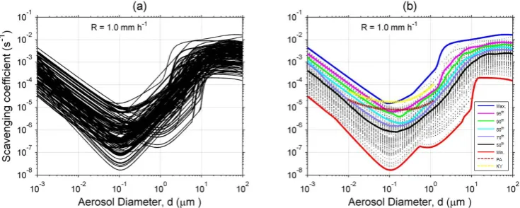
formu-las, respectively, as listed in Tables 1, 2, and 3). Note that the product-term formulas were originally generated from a wide range of rain types such as “widespread”, convective, thunderstorm, and hurricane. Figure 1 shows the results for a precipitation intensityR of 1.0 mm h−1as an example. The predicted3rain values differ by one order of magnitude for ultrafine (e.g., < 0.01 µm) and giant (e.g., > 10 µm) aerosol particles and by nearly two orders of magnitude for particles in the diameter range from 0.01 to 10 µm.
Next, following step 2 from Sect. 2, we found that two groups of3rainprofiles had different shapes from the rest of the profiles for all of the precipitation intensities considered in this study. One group predicts much higher3rainvalues for aerosol particles larger than 0.5 µm (see group of yellow lines in Fig. 1a) and the other group predicts much lower3rain val-ues for aerosol particles larger than 1.0 µm (see group of red lines in Fig. 1a). The first group was identified to be caused by the use of the E(d, Dp) formula of Park et al. (2005) and the second group by the use of theE(d, Dp)scheme of Ackerman et al. (1995).
802 X. Wang et al.: Development of a new semi-empirical parameterization
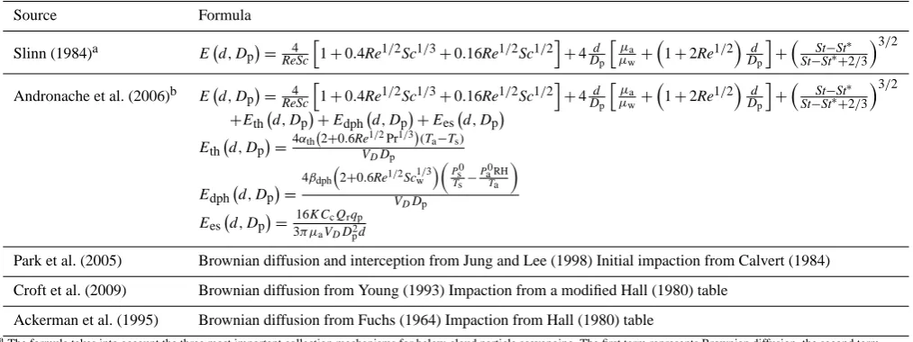
Table 1. List of semi-empirical formulas for raindrop–aerosol particle collection efficiencyE(d, Dp). Symbols used in Tables 1–9 and their
units are defined in Table E1 in Appendix E.
Source Formula
Slinn (1984)a E d, Dp=ReSc4
h
1+0.4Re1/2Sc1/3+0.16Re1/2Sc1/2i+4Dd
p
hµ
a
µw+
1+2Re1/2Dd
p
i
+ St−St∗
St−St∗+2/3
3/2
Andronache et al. (2006)b E d, Dp=ReSc4
h
1+0.4Re1/2Sc1/3+0.16Re1/2Sc1/2i+4Dd
p
hµ
a
µw+
1+2Re1/2Dd
p
i
+ St−St∗
St−St∗+2/3
3/2
+Eth d, Dp+Edph d, Dp+Ees d, Dp
Eth d, Dp=4αth2
+0.6Re1/2Pr1/3 (Ta−Ts)
VDDp
Edph d, Dp= 4βdph
2+0.6Re1/2Sc1/3 w
P0 s
Ts−
Pa RH0
Ta
VDDp
Ees d, Dp
= 16KCcQrqp
3π µaVDD2pd
Park et al. (2005) Brownian diffusion and interception from Jung and Lee (1998) Initial impaction from Calvert (1984)
Croft et al. (2009) Brownian diffusion from Young (1993) Impaction from a modified Hall (1980) table
Ackerman et al. (1995) Brownian diffusion from Fuchs (1964) Impaction from Hall (1980) table
aThe formula takes into account the three most important collection mechanisms for below-cloud particle scavenging. The first term represents Brownian diffusion, the second term
represents interception, and the third term represents inertial impaction. Re is the Reynolds number: Re=DpVDρa/2µa. Sc is the Schmidt number: Sc=µa/ρaDdiff, where Ddiff=kbTaCc/(3π µad)with the Cunningham correction factor:Cc=1+2λda
1.257+0.4 exp
−1.1d
2λa
. St is the Stokes number: St=2τ VD−vd
/Dpwith the characteristic
relaxation time of a particle:τ= ρp−ρa
d2Cc/18µa. St∗is the critical Stokes number expressed asSt∗=1.2+ln(1+Re)/12 1+ln(1+Re) .
bThe formula takes into account three additional collection mechanisms due to thermophoresisE
th(d, Dp), diffusiophoresisEdph(d, Dp), and electrostatic forcesEes(d, Dp)based on
Slinn (1984). The parameterαthand the Prandtl number Pr inEth(d, Dp)are defined asαth=
2Ccka+5λa/Dpkpka
5P1+6λa/Dp2ka+kp+10λa/Dpkp, and Pr=cpµa/ka, respectively. The parameterβdph
and the Schmidt number for water ScwinEdph(d, Dp)are defined asβdph=TaDdiffwaterP
q
Mw
Ma, and Scw=µa/ρaDwaterdiff, respectively. The parameterKinEes(d, Dp)is set as
9×10⁹(in Nm2C−2).Qrandqpare the mean charges on the raindrop and on the aerosol particle (in Coulomb, C), respectively, with opposite sign, and are parameterized as
Qr=aαD2pandqp=aαd2witha=0.83×10⁻⁶andα(C m−2), an empirical parameter, in the range of 0–7 corresponding to cloud charges from neutral to highly electrified clouds.
threshold in the inertial impaction mechanism, which leads to an additional contribution of inertial impaction toE(d, Dp) for particles smaller than 3 µm in diameter. In fact, inertial impaction can only occur for particles with a Stokes num-ber above the critical Stokes numnum-ber, which is close to 1.2. The corresponding threshold diameter is close to 3 µm for a unit-density particle and a 1 mm raindrop (Phillips and Kaye, 1999; Loosmore and Cederwall, 2004). Thus,3rain calcu-lated using the E(d, Dp) formula of Park et al. (2005) is believed to be an overestimation for particles with diame-ters from 0.5 to 3 µm. TheE(d, Dp)scheme of Ackerman et al. (1995), on the other hand, considers the collection mech-anisms of Brownian diffusion, convective Brownian diffu-sion enhancement, and inertial impaction. In this scheme, the required collision efficiency values are interpolated from a look-up table from Hall (1980). The table, however, only covers collector (raindrop) sizes of 10–300 µm in radius col-liding with aerosol particles (collected particles) with size ratios (the so-called p-ratio) from 0.05 to 1.0. There are no data available for collectors larger than 300 µm in radius, a size range that has appreciable concentrations in medium to heavy rain, or for particles with size ratios less than 0.05, which can include particles from 0.5 to 10 µm in radius. As well, collision efficiencies for collectors smaller than 30 µm were later found to be underestimated (Vohl et al., 2007). These deficiencies appear to be the main causes of the lower
values of3rainfor particles in the diameter range from 1.0 to 10.0 µm compared to the rest of the3rainformulas.
The above examination suggests that the two groups of 3rain profiles that used the E(d, Dp) formulation of Park et al. (2005) and Ackerman et al. (1995) were not as real-istic as the rest of the 3rain profiles. We thus removed the 3rainprofiles based on theE(d, Dp)formulation of Park et al. (2005) from further consideration since there was no easy way to fix the problem. We noticed, however, that Vohl et al. (2007) had updated the Hall (1980) table with new ex-perimental results that provided more realistic collision effi-ciencies for wider size ranges for both collector and collected particles. Thus, we chose to keep the3rainprofiles based on theE(d, Dp)scheme of Ackerman et al. (1995) for further analysis, but these were modified profiles based on the up-dated collision efficiency table of Vohl et al. (2007) in place of the Hall (1980) table.
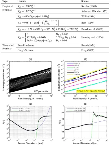
Fig. 1. Size-resolved scavenging coefficients for rain conditions: (a)3rain calculated using Eq. (2) from a total of 400 combinations of
differentE(d, Dp),N (Dp), andVDformulas listed in Tables 1, 2, and 3, respectively. The yellow group uses theE(d, Dp)formula of Park
et al. (2005) and the red group uses theE(d, Dp)formula of Ackerman et al. (1995); the black group includes all the other combinations;
(b) same as in (a) but with the yellow group removed and the red group using the modifiedE(d, Dp)formula of Ackerman et al. (1995)
(reduced to a total of 320 combinations); (c) minimum, maximum, and five percentile3rainprofiles (colored lines) based on ensemble of
profiles from (b), where dots are the data from (b); (d) lines are the same as (c) and symbols are experimental data reviewed in Wang et al. (2010). Also shown in (d) are one empirical3rainparameterization of Laakso et al. (2003) (denoted by LA; see Appendix A) and one
semi-empirical3rainparameterization of Henzing et al. (2006) (denoted by HS; see Appendix B), which is an empirical fit to theoretically
calculated3rainvalues.
3rain profiles were also comparable to the other 2403rain profiles that used differentE(d, Dp)formulas (see the large group of black lines in Fig. 1b). Thus, it is recommended that the Hall (1980) table should be used with caution in the parameterization of3rainin CTMs.
Using the 3203rainprofiles shown in Fig. 1b, we identi-fied a number of percentile values of3rainfor each aerosol particle diameter. These maximum, 95th-, 90th-, 80th-, 70th-, and 50th-percentile, and minimum3rain profiles are shown in Fig. 1c. Note that the dots in this panel correspond to the original3rainvalues shown in Fig. 1b and the lines are the calculated percentile 3rain profiles. Note also that the per-centile profiles in Fig. 1c may not match exactly with any of the3rainprofiles shown in Fig. 1b, but they represent the range and distribution of the ensemble of all theoretical3rain values across the range of different aerosol particle sizes.
In Fig. 1d the percentile3rainprofiles are compared with the available3rainmeasurements and one empirical formula
804 X. Wang et al.: Development of a new semi-empirical parameterization
Table 2. List of raindrop number size distribution (N (Dp)) formulas. The general forms of the (a) exponential, (b) gamma,
and (c) log-normal distributions are commonly written as N (Dp)=N0eexp −βeDp, N (Dp)=N0gDγpexp −βgDp, and N Dp=
Nt ot al √
2π Dpln(σD) exp
− ln(Dp)−ln(Dmean)
2 2(ln(σD))2
, respectively. See Table E1 in Appendix E for definitions of other symbols and units.
Raindrop number
size spectrum Formula definition Rain type Source
Exponential N0e=0.08, βe=41R−0.21 Widespread Marshall and Palmer (1948)
distributions(a)
N0e=0.30, βe=57R−0.21 Drizzle Joss et al. (1968)
N0e=0.014, βe=30R−0.21 Thunderstorm Joss et al. (1968)
N0e=0.07R0.37, βe=38R−0.14 Thunderstorm Sekhon and Srivastava (1971)
N0e=0.071M0.648, βe=
10−6ρ wπ N0e
M
0.25
Convective Zhang et al. (2008)
M=0.0626R0.913
Gamma N0g=168.53R−0.384 Widespread de Wolf (2001)
distributions(b) γ=2.93, βg=53.8R−0.186
N0g=6.36×10 −4M
d4 0
1
d0
2.5
Hurricane Willis (1984)
γ=2.50, βg=5.57/d0
d0=0.157M0.168, M=0.062R0.913
N0g=5.1285×10 −4M
d4 0
1
d0
2.16
Hurricane Willis and Tattelman (1989)
γ=2.16, βg=5.588/d0
d0=0.1571M0.1681, M=0.062R0.913
Log-normal Ntotal=1.72×10⁻⁴R0.22, Dmean=0.072R0.23 Widespread Feingold and Levin (1986)
distributions(c) σD= 1.43–3.0×10⁻⁴R
Ntotal=1.94×10⁻⁴R0.30, Dmean=0.063R0.23 Widespread Cerro et al. (1997)
σD=e √
0.191−1.1×10⁻²·ln(R)
falls into the lower range of the ensemble of available theo-retical3rainvalues.
The large differences in 3rain between the in situ field-derived values and those from the controlled outdoor exper-iment and between the field experexper-iments and the theoretical formulations are caused by many different factors. Some of the differences might reflect the uncontrolled real-world sit-uation while others are due to experimental errors and to er-rors in the theoretical formulations (Khain and Pinsky, 1997; Maria and Russell, 2005; Andronache et al., 2006; Wang et al., 2011; Quérel, 2012; Quérel et al., 2013). Choosing the upper range of theoretical 3rain values for applications in CTMs appears to be a reasonable choice because these values are only slightly higher than the corresponding values from the controlled outdoor experiment but are still lower than val-ues from the majority of field experiments. Thus, the 90th percentile of the range of the ensemble of theoretical3rain profiles was chosen for further analysis and parameterization development.
Moving to step 3 in Sect. 2, we repeated the calculation of 3rain with Eq. (2) for all of the 320 combinations of
product-term formulas for each of 37 different precipitation intensitiesR, which covered the range of values from 0.01 to 100 mm h−1 and were uniformly distributed logarithmi-cally (same as the tick values shown inx axis of Fig. 2b). Furthermore, 90th-percentile 3rain values were then calcu-lated from the ensemble of theoretical3rainprofiles for each aerosol particle diameter bindand every precipitation inten-sityR. These 90th-percentile3rain data are plotted against precipitation intensity in Fig. 2a as a set of 100 lines, with each line representing one aerosol particle diameter and in the form of3rainvs.R.
Regression analysis suggests that for each aerosol particle diameter (i.e., each individual line in Fig. 2a), there exists a strong linear relationship between log10(3rain)and log10(R), or in other words a power-law relationship between3rainand R, which can be expressed as
log10(3(d, R))=log10(A(d))+B(d)(log10R), (4)
Table 3. List of empirical and theoretical raindrop terminal velocity (VD)formulas.
Type Formula Source
Empirical VD=1300D0p.5 Kessler (1969)
formulas
VD=1767D0p.67 Atlas and Ulbrich (1977)
VD=4854Dpexp −1.95Dp Willis (1984)
VD=958
1−exp
− Dp
0.171
1.147
Best (1950)
VD= −10.21+4932Dp−9551Dp2+7934D3p−2362Dp4 Brandes et al. (2002)
VD=
0
4323(Dp−0.003)
965−1030 exp −6Dp
Dp≤0.003
0.003≤Dp≤0.06
Dp>0.06
Henzing et al. (2006)
Theoretical Beard’s scheme Beard (1976)
formulas
Feng’s Scheme Feng (2007)
Fig. 2. (a) 90th-percentile3rainprofiles as a function of precipitation intensityRderived from an ensemble of 3203rainrealizations for
100 particle diameters (a total of 100 lines); (b) linear regression best-fit lines for the 90th-percentile3raindata (symbols) from (a) for
seven aerosol particle diameters; (c) values (symbols) ofyinterceptA(d)from the log-linear regressions for 100 particle diameters and their polynomial best-fit curves (lines); and (d) same as in (c) but for the slopeB(d)of the log-linear regressions.
Linear regression analysis based on Eq. (4) was performed for all 100 lines and the squares of the resulting correla-tion coefficients were very high, ranging from 0.9963 to 1.0. Figure 2b shows seven of these regression lines for seven
806 X. Wang et al.: Development of a new semi-empirical parameterization
Fig. 3. Parameterized size-resolved3rainprofiles using Eqs. (5), (6), and (7) (solid lines) and the original 90th-percentile3raindata (symbols)
(a) and their percentage differences (b) for five different precipitation intensities.
panel that both the slope of the regression lines (B(d))and itsyintercept (log10A(d))may vary with aerosol particle di-ameter. Note, however, that theyintercept does not cross the yaxis shown in Fig. 2b because the actualRvalue instead of log10(R)is used for thexaxis. But according to Eq. (4),A(d) equals3rain(d, 1) (i.e., whenR=1.0 mm h−1), soA(d) val-ues are also readily available. The resultingA(d)andB(d) values are plotted in Fig. 2c and d, respectively, for each of 100 aerosol particle diameters.
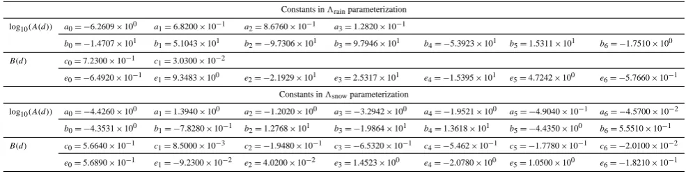
SinceA(d)andB(d)correspond at this stage to sets of dis-crete data, a least-square polynomial curve-fitting technique was used to fit these power-law coefficient data and parame-terizeA(d)andB(d)as continuous functions of aerosol par-ticle diameter. Due to the abrupt change of the values of both A(d)andB(d)at particle diameters between 1 and 2 µm, the particle diameter range of each of the two data sets was split into two contiguous segments for separate but more accurate fitting. After many tests, the separation point of the two seg-ments was determined to be 1.97 µm forA(d)(see Fig. 2c) and 1.94 µm forB(d)(see Fig. 2d). We thus chose 2.0 µm to be the separation point for both theA(d)andB(d)curve fits. After some experimentation, the following polynomial functions (up to sixth order) were selected for fitting the four segments:
log10(A(d))=
a0+a1(log10d)+a2(log10d)2
+a3(log10d)3 d≤2.0 µm
b0+b1(log10d)+b2(log10d)2 +b3(log10d)3+b4(log10d)4
+b5(log10d)5+b6(log10d)6 d >2.0 µm
(6)
B(d)=
c0+c1(log10d) d≤2.0 µm e0+e1(log10d)+e2(log10d)2
+e3(log10d)3+e4(log10d)4
+e5(log10d)5+e6(log10d)6 d >2.0 µm.
(7)
Note that the unit ofdis µm, and the above equations should be applied to wet aerosol diameter. The empirical best-fit coefficients that were obtained for the above equations are listed in Table 8.
A comparison of3rainvalues predicted by the new param-eterization described by Eqs. (5), (6), and (7) with the data used for developing the parameterization (the 90th-percentile 3rain(d, R)values) is shown in Fig. 3a for five different pre-cipitation intensities. Very good agreement is evident for the full range of aerosol particle size and full range of precip-itation intensity. To further examine the comparison shown in Fig. 3a, the relative error between3rain values from the new parameterization and the original 90th-percentile values was also calculated (Fig. 3b). The relative error was within 10 % for most of the aerosol particle sizes, except for the 2– 6 µm diameter range for which the error could be larger than 30 %. The largest relative errors corresponded to the aerosol particle diameters where3rainincreased abruptly with parti-cle diameter. It should also be noted that various partiparti-cle-size separation points were tested for the separate fits of Eqs. (6) and (7) (e.g., from 1.9 to 2.2 µm), and a separation point of 2.0 µm does lead to the minimum relative errors for most aerosol sizes.
To gain an idea of howA(d)andB(d)in Eqs. (6) and (7) would differ if3rain(d, R)values other than 90th-percentile ones had been used, a separate empirical fitting was per-formed using 50th-percentile values. It was found thatB(d) values did not change by very much, whereas A(d)values differed by one order of magnitude. As noted above,B(d) represents the rate of change of3rain(d, R) for changes of R while A(d)represents the 3rain(d, R) value whenR=
1.0 mm h−1. This means that 3rain(d, R) for the 90th and 50th percentiles vary similarly with changes in R, but the magnitude of the 90th-percentile3rain(d, R)is much larger than the 50th-percentile3rain(d, R).
Table 4. List of semi-empirical formulas for snow particle–aerosol particle collection efficiencyE.
Source Formula
Slinn (1984)a E (d, λ)=(Sc1)αλ+h1−exp(−(1+Re1λ/2))(d/2)2
λ2
i
+ St−St∗
St−St∗+2/3
3/2
Murakami et al. (1985)b E (d, Dm)=π D48DmdiffV
D(0.65+0.44Sc
1/3Re1/2)+28.5I1.186+ S1−S2
S2exp(S1t0)−S1exp(S2t0)
2
Dick (1990)c E (d, Dm)=3π dµ2mVaDDm+Pe4(1+0.4Re1/6Pe1/3) aλis the characteristic capture length andα
λis an empirical constant. Bothλandαλdepend on the shape of snow particles (e.g., sleet/graupel, rimed crystals, powder snow, dendrite, tissue paper, and camera film). Reλis the Reynolds number corresponding to the specificλ, Sc is the Schmidt number: Sc=µa/ρaDdiff, St is the Stokes number, and St∗is the critical Stokes number: St∗=
1.2+(1/12)ln 1+Reλ
1+ln 1+Reλ .
bThe formula is for snow aggregates. The Reynolds number of a snow particle is defined as Re=D
mVDρa/µa, Sc is the Schmidt number, andIis the size ratiod/DcwithDcthe characteristic length of the snow particle. The third term is the theoretical solution of a simplified flow model by Ranz and Wong (1952), involving parametersS1,S2andt0, and it can be simplified to exp( −0.11
St1/2−0.25)if St≥1/16, or to 0 if St < 1/16 (Feng, 2009). cPe is the Peclet number: Pe=D
mVD/Ddiffand Re is the Reynolds number: Re=DmVDρa/2µa.
Table 5. List of exponential snow particle number size distribution (N (Dp))formulas. Note that actual snow particle sizeDm(cm) was used
in Scott (1982) (see Appendix A in Zhang et al., 2013), whereasDpwas used in other formulas.
N (Dp)=N0eexp −βeDp
Source N0e[cm−4] βe[cm−1]
Marshall and Palmer (1948) 0.08 βe=41R−0.21
Scott (1982) 0.5 M=0.37R0.94
βe=20.7M−0.33=28.8R−0.31
Gunn and Marshall (1958) N0e=0.038R−0.87 βe=25.5R−0.48
Sekhon and Srivastava (1970) N0e=0.025R−0.94 βe=22.9R−0.45
parameterization does not exactly match any of the exist-ing theoretical profiles considered, but for all aerosol parti-cle diameters its values will lie within the upper range of an ensemble of theoretical3(d)values obtained from all pos-sible combinations of existing product-term formulas. The new parameterization is designed for use in CTMs to de-scribe below-cloud scavenging of size-resolved aerosol par-ticles. We believe it to be a reasonable first-order approxi-mation for any precipitation conditions, either stratiform or convective, considering that precipitation intensity and pre-cipitation type (i.e., rain or snow) are likely to be the only precipitation information available in many CTMs (e.g., in-formation on different rain types or droplet size distributions may not be available).
3.2 3snow
The development of the new semi-empirical parameteriza-tion for3snow follows the same approach described above for3rain. The first step was to calculate an ensemble of the-oretical3snowprofiles across the aerosol particle size spec-trum using Eq. (2) for a precipitation intensity of 1.0 mm h−1 for all possible combinations of the product terms listed in Tables 4–7. There are threeE(d, Dp), fourN (Dp), eightVD,
and fourAformulas available in the literature related to snow particles, but some of theVD formulas were only
applica-ble to specific snow types. Thus, a total of 168 combinations of these product-term formulas were used to calculate3snow profiles (see Fig. 4a). Note that these formulas cover four habit types of snow crystals – spherical ice crystals, dendritic snow plates, columnar ice crystals, and graupel particles (see Table 7), all of which occur frequently in nature (e.g., Hobbs et al., 1972).
808 X. Wang et al.: Development of a new semi-empirical parameterization
1
Fig. 4. Size-resolved scavenging coefficient under snow conditions: (a)3snowcalculated using Eq. (2) from a total of 168 combinations of
E(d, Dp),N (Dp),VDandAlisted in Tables 4, 5, 6, and 7, respectively; and (b) minimum, maximum, and five percentile3snowprofiles
(colored lines) based on ensemble of profiles from (a), where dots are the data from (a). Also shown in (b) are two empirical3snowformulas
of Paramonov et al. (2011) and Kyrö et al. (2009) (Appendices C and D, respectively).
Table 6. List of empirical and theoretical snow particle terminal velocity (VD)formulas.Xis the best number:X= 2mgρaD
2 m
Aµ2 a
,α,β,δ, and
σare empirical constants (see Table 7), anda1andb1are described as functions ofX(see Mitchell and Heymsfield, 2005).
Source VDformula Particle shape
Langleben (1954) VD=207.0D0p.310 plane dendrite
Jiusto and Bosworth (1971) VD=104.9D0m.206 plane dendrite
Locatelli and Hobbs (1974) VD=64.80D0m.257 plane dendrite
Molthan et al. (2010) VD=110.1D0m.145 plane dendrite
Jiusto and Bosworth (1971) VD=153.0D0m.206 column
Matson and Huggins (1980) VD=1145Dp0.500 graupel
Mitchell (1996) VD=DRemµρaa any shape
Re=
0.04394X0.970,0.01< X≤10.0 0.06049X0.831,10.0< X≤585 0.2072X0.638,585< X≤1.56×10⁵ 1.0865X0.499,1.56×105< X≤108
Mitchell and Heymsfield (2005) VD=avDbmv,Re=a1Xb1, m=αDβm, A=δDσm any shape
av=a1
µa
ρa
(1−2b1)2αg ρaδ
b1
, bv=b1(β−σ+2)−1
formulas together without explicit consideration of snow par-ticle shape. Thus, all of the values in Fig. 4a were used for further analysis. Similar to Fig. 1c, the range and per-centile values of 3snow were also generated as shown in Fig. 4b. Also plotted are two field-derived empirical for-mulas for 3snow, one from Paramonov et al. (2011) (Ap-pendix C) and one from Kyrö et al. (2009) (Ap(Ap-pendix D), but it should be noted that both formulas are more appli-cable to weaker snowfall intensities (e.g., 0.1–0.2 mm h−1) than the intensity assumed in Fig. 4b (1 mm h−1) and are only valid for aerosol particle sizes in 0.01–1.0 µm diameter range. Figure 4b shows that the upper range of the theoret-ical3snowprofiles calculated assuming a snowfall intensity of 1 mm h−1are of the same order of magnitude as the lim-ited field data, which were observed under mostly weaker
snowfall intensities. The theoretical3snowprofiles would be smaller than the experimental data if the same snowfall in-tensity as observed in the field were to be used for the cal-culation of 3snow using Eq. (2). To be consistent with the choice made for 3rain, the 90th percentile of the ensemble of all theoretical3snowformulations at each aerosol particle diameter was also used to develop the new parameterization for 3snow. However, the evidence supporting this choice is somewhat weaker for 3snow than for 3rain due to the very limited field data for snow scavenging cases.
Fig. 5. Same as in Fig. 2 except for3snow.
Table 7. Snow particle shapes considered in this study and their mass (m) and cross-sectional area (A) formulas.
Snow particle Mass Cross-sectional area shape m=αDmβ[g] A=δDmσ [cm2]
Spheres m=0.0524Dm3.00,a A=0.7854Dm2.00,a
Dendrites m=0.0022Dm2.19,b A=0.2285Dm1.88,c
Columns m=0.0450Dm3.00,b A=0.0512Dm1.41,d
Graupel m=0.0490Dm2.80,e A=0.5000Dm2.00,e aObtained fromm=ρ
s(π/6)D3mandA=(π/4)D2m, withρs=0.1g cm−3.
bFrom Woods et al. (2008).
cFrom Mitchell (1996) for “aggregates of side planes”. dFrom Mitchell (1996) for “rimed long columns”. eFrom Mitchell (1996) for “lump graupel”.
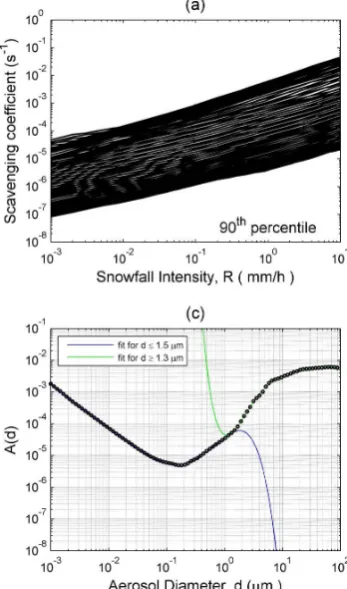
equivalent to 1 mm of rain, a different range of precipitation intensities was used to generate the3snowensemble data set than that used in the3rain case. 90th-percentile3snow val-ues for each aerosol particle diameter were then extracted for each precipitation intensity and are plotted in Fig. 5a, where again each line corresponds to a fixed aerosol particle di-ameter. The relationship between log10(3snow)and log10(R) can also be described by Eq. (4). Linear regressions were
again calculated, and the squares of the correlation coeffi-cients of the 100 regressions were again very high, ranging from 0.9736 to 0.9997. Seven of the 100 regression lines to-gether with the data points being fit are plotted in Fig. 5b as examples.
The same approach described in Sect. 3.1 was also used here to generate log10(A(d))andB(d)values (Fig. 5c and d) and to conduct least-squares polynomial curve-fitting to pa-rameterize log10(A(d))andB(d)for alldvalues. Again, the data sets were split into two contiguous segments for separate fitting. Multiple intersections between the two fitting func-tions were found for both the log10(A(d))andB(d)cases. This time a final separation point was chosen at a particle diameter of 1.44 µm because this value produced the mini-mum relative errors between the parameterized and the origi-nal theoretical3snowvalues. The polynomial fitting formulas for the snow case are shown below and their corresponding empirical best-fit coefficients are listed in Table 8.
log10(A(d))=
a0+a1(log10d)+a2(log10d)2 +a3(log10d)3+a4(log10d)4
+a5(log10d)5+a6(log10d)6 d≤1.44 µm b0+b1(log10d)+b2(log10d)2
+b3(log10d)3+b4(log10d)4
+b5(log10d)5+b6(log10d)6 d >1.44 µm
810 X. Wang et al.: Development of a new semi-empirical parameterization
Table 8. Empirical constants in the formulations of log10(A(d))andB(d)for3rainand3snowparameterizations.
Constants in3rainparameterization
log10(A(d)) a0= −6.2609×100 a1=6.8200×10⁻¹ a2=8.6760×10⁻¹ a3=1.2820×10⁻¹
b0= −1.4707×101 b
1=5.1043×101 b
2= −9.7306×101 b
3=9.7946×101 b
4= −5.3923×101 b
5=1.5311×101 b
6= −1.7510×100
B(d) c0=7.2300×10⁻¹ c1=3.0300×10⁻²
e0= −6.4920×10⁻¹ e1=9.3483×100 e2= −2.1929×101 e3=2.5317×101 e4= −1.5395×101 e5=4.7242×100 e6= −5.7660×10⁻¹ Constants in3snowparameterization
log10(A(d)) a0= −4.4260×100 a1=1.3940×100 a2= −1.2020×100 a3= −3.2942×100 a4= −1.9521×100 a5= −4.9040×10⁻¹ a6= −4.5700×10⁻²
b0= −4.3531×100 b1= −7.8280×10⁻¹ b2=1.2768×101 b3= −1.9864×101 b4=1.3618×101 b5= −4.4350×100 b6=5.5510×10⁻¹
B(d) c0=5.6640×10⁻¹ c1=8.5000×10⁻³ c2= −1.9480×10⁻¹ c3= −6.5320×10⁻¹ c4= −5.462×10⁻¹ c5= −1.7780×10⁻¹ c6= −2.0100×10⁻²
e0=5.6890×10⁻¹ e1= −9.2300×10⁻² e2=4.0200×10⁻² e3=1.4523×100 e4= −2.0780×100 e5=1.0500×100 e6= −1.8210×10⁻¹
B(d)=
c0+c1(log10d)+c2(log10d)2 +c3(log10d)3+c4(log10d)4
+c5(log10d)5+c6(log10d)6 d≤1.44 µm e0+e1(log10d)+e2(log10d)2
+e3(log10d)3+e4(log10d)4
+e5(log10d)5+e6(log10d)6 d >1.44 µm
(9)
A comparison of the new parameterization described by Eqs. (5), (8), and (9) with the 3snow values from Fig. 5a is shown in Fig. 6a for five different precipitation intensi-ties and the relative error from this comparison is shown in Fig. 6b. Reasonably good agreement was observed for the full range of aerosol particle size and full range of precipi-tation intensity. The relative error was within 30 % for most aerosol particle sizes, except for the 1–4 µm diameter range, for which the error could be as large as 50 %. Considering the very large range (i.e., two orders of magnitude or larger) of the existing theoretical3snowvalues (cf., Fig. 4), an un-certainty of 50 % or a factor of 2 in the parameterized3snow values should be acceptable.
4 Discussion
4.1 Power-law relationship between3andR
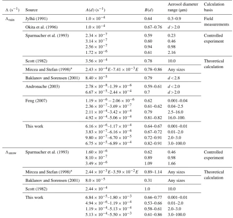
A power-law relationship between the size-resolved3rainor 3snowparameters and precipitation intensityRfor each par-ticle diameterd was identified in Sect. 3 and was used in the development of the new parameterization. The finding of such a power-law relationship is not surprising since many earlier theoretical and experimental studies also suggested the existence of such a relationship, although most of the earlier studies focused on bulk3instead of size-resolved3 (Mircea and Stefan, 1998; Andronache, 2003; Duhanyan and Roustan, 2011). A brief comparison of the results from the present study with earlier studies in terms of the power-law parameters is provided in Table 9 and presented below.
Early investigations reviewed by McMahon and Denison (1979) and more recent theoretical considerations (e.g., Scott, 1982; Mircea and Stefan, 1998; Andronache,
2003) as well as field and experimental studies (Jylhä, 1991; Okita et al., 1996; Sparmacher et al., 1993) have suggested that the exponent B had values in the range of 0.59–0.94 for3rainand 0.3–1.14 for3snow(see Table 9 and the reviews of Sportisse, 2007, and Duhanyan and Roustan, 2011). The field measurements by Jylhä (1991) and Okita et al. (1996) reported B values of 0.64–0.76. Sparmacher et al. (1993) fitted their experimental 3 data from their controlled outdoor study with a power-law relationship and obtainedB(d)values of 0.59, 0.60, 0.94, and 0.61 for four selected aerosol particle diameters of 0.23, 0.46, 0.98, and 2.16 µm, respectively, for rain scavenging and values of 0.62, 0.89, and 1.09 for three selected aerosol particle diameters of 0.46, 0.98, and 1.66 µm, respectively, for snow scavenging. The B values obtained from theoretical derivations (Scott, 1982; Mircea and Stefan, 1998; Baklanov and Sorensen, 2001; Andronache, 2003; Feng, 2007) ranged from 0.59 to 0.86 for submicron particles and from 0.7 to 0.86 for coarse-mode particles for rain scavenging and from 0.31 to 1.14 for both submicron and for coarse-mode particles for snow scavenging with different habit types of snow crystals. However, the two most recent field studies on snow scavenging (Kyrö et al., 2009; Paramonov et al., 2011) did not identify a clear dependency of3snowonR. As discussed in Zhang et al. (2013), we speculated that this might be due to the small range of snowfall intensities sampled in these experiments.
Table 9. List of below-cloud3rainand3snowparameterizations from literature expressed as3(d, R)=A(d)RB(d)(where3is in units of
s−1).
Aerosol diameter Calculation
3(s−1) Source A(d)(s−1) B(d) range (µm) basis
3rain Jylhä (1991) 1.0×10⁻⁴ 0.64 0.3–0.9 Field
Okita et al. (1996) 1.0×10⁻⁴ 0.67–0.76 d> 2.0 measurements Sparmacher et al. (1993) 2.34×10⁻⁷ 0.59 0.23 Controlled
3.14×10⁻⁷ 0.60 0.46 experiment
2.56×10⁻⁷ 0.94 0.98
1.72×10⁻⁶ 0.61 2.16
Scott (1982) 3.56×10⁻⁴ 0.78 10.0 Theoretical
Mircea and Stefan (1998)∗ 2.43×10−4E–7.41×10⁻³E 0.78–0.86 Any sizes calculation Baklanov and Sorensen (2001) 8.40×10⁻⁵ 0.79 d< 2.8
Andronache (2003) 2.78×10⁻⁸–1.39×10⁻⁶ 0.59–0.61 d< 2.0 6.67×10⁻⁵–2.44×10⁻⁴ 0.7 d> 2.0 Feng (2007) 1.19×10⁻⁶−2.06×10⁻⁶ 0.62 0.001–0.04
2.36×10⁻⁷–3.69×10⁻⁷ 0.61–0.62 0.04–2.5 2.11×10⁻⁴–3.42×10⁻⁴ 0.79 2.5–16.0 4.92×10⁻⁴–5.06×10⁻⁴ 0.81–0.82 16.0–100. This work 6.16×10⁻⁶–1.17×10⁻⁴ 0.64–0.67 0.001–0.01
3.83×10⁻⁷–6.16×10⁻⁶ 0.67–0.72 0.01–2.0 9.80×10⁻⁷–6.70×10⁻⁵ 0.72–0.91 2.0–3.0 6.75×10⁻⁵–6.89×10⁻⁴ 0.82–0.91 3.0–100.0
3snow Sparmacher et al. (1993) 1.60×10⁻⁶ 0.62 0.46 Controlled
8.10×10⁻⁷ 0.89 0.98 experiment
3.49×10⁻⁶ 1.09 1.66
Mircea and Stefan (1998)∗ 2.44×10−3E–3.59×10⁻²E 0.89–1.14 Any sizes Theoretical Baklanov and Sorensen (2001) 8.0×10⁻⁵ 0.31 Any sizes calculation
Scott (1982) 2.44×10⁻⁴ 1.0 10.0
This work 6.84×10⁻⁵–1.80×10⁻³ 0.66–0.77 0.001–0.01 4.94×10⁻⁶–1.19×10⁻⁴ 0.53–0.66 0.01–2.0 1.19×10⁻⁴–5.13×10⁻⁴ 0.58–0.61 2.0–3.0 5.13×10⁻⁴–5.50×10⁻³ 0.61–0.86 3.0–100.0
∗Eis the collection efficiency and assumed to be a constant for a given precipitation distribution and aerosols types.
As noted in Sect. 3.1 the parameter A(d) equals 3(d) whenR=1.0 mm h−1. Therefore, the values ofA(d)should be similar to the upper range of those in the theoretical for-mulas and lower than those in the field-data-based empirical ones given the design decisions made in the development of the new parameterization. A comparison ofA(d)values from the new parameterization with those found in the literature (Table 9) supports this hypothesis.
4.2 Relative magnitudes of3rainand3snow
812 X. Wang et al.: Development of a new semi-empirical parameterization
Fig. 6. Same as in Fig. 3 except for3snow.
Fig. 7. (a) The ratio of parameterized3snow–3rainas a function of precipitation intensityR(liquid water equivalent) for 100 aerosol particle
diameters (100 lines in total). The groups of blue, yellow, and green lines correspond to aerosol particle diameters < 0.1 µm, 0.1–5.0 µm, and > 5.0 µm, respectively; (b) the ratio of parameterized3snow–3rainas a function of aerosol particle diameterdfor four selected valuesR.
the new scheme might be expected to be larger than values of3rainfrom the new scheme for equivalent precipitation in-tensity. To obtain a quantitative measure of the relative mag-nitudes of3rainand3snowfor the new parameterization, the ratios of3snowto3rainas a function of precipitation intensity were calculated for all 100 aerosol particle diameters.
Figure 7a shows that the magnitude of 3snow is higher than that of3rain for the same precipitation intensity by a factor ranging from 3 to 300, depending on aerosol particle size and precipitation intensity. The ratio of3snowto3rainis the highest for medium particle sizes (i.e., 0.1 <d< 5.0 µm; shown as yellow lines) and is the lowest for coarse and giant particles (e.g.,d> 5.0 µm; shown as green lines). The largest ratios were found for a particle diameter of about 2.0 µm for allRvalues. However, the lowest ratios were found to occur for a particle diameter of 100 µm for smallR values (lowest green line) and a particle diameter around 4.0 µm for large Rvalues (lowest yellow line). The dependence of the3snow to3rainratio on particle diameter can be better seen in Fig. 7b for selectedRvalues. The ratio decreases with increasingR for medium-size particles (yellow lines in Fig. 7a), increases
with increasingR for ultrafine particles (some of the blue lines in Fig. 7a), and only change slightly with increasingR for giant particles (e.g.,d> 10 µm; some of the blue lines in Fig. 7a).
X. Wang et al.: Development of a new semi-empirical parameterization 813
2 Fig. 8. Percentage differences in3from the use of different temperature and pressure values for (a) rain and (b) snow scavenging versus base case. A precipitation intensity of 1.0 mm h−1was assumed, and the base case refers to the ambient conditions used to develop the new
3parameterization (i.e.,p=1013.25 hPa;T =15◦C for rain scavenging andT = −10◦C for snow scavenging).
the larger cross-sectional areas of snow particles. Thus, the ratio between the snow and rain scavenging coefficients in Fig. 7 increases in the particle diameter range between 0.1 to 1.0 µm. The second significant difference relates to the abrupt transition of3rainfrom an interception regime to an inertial-impaction regime at a particle diameter of about 2 µm (Fig. 1d). For particle diameters larger than 2 µm,3rain in-creases more quickly withd than does3snow. As a result, the3snowto3rainratio decreases quickly with increasingd until leveling off for particle diameters close to 10 µm.
Some previous studies also support the result that snow scavenging is more effective than rain scavenging for equiv-alent precipitation amounts. Several field studies carried out before the 1980s found that snow scavenging of aerosols was 28 to 50 times more efficient than rain scavenging based on the equivalent water content of the precipitation (Reiter, 1964; Carnuth, 1967; Reiter and Carnuth, 1969; Graedel and Franey, 1975). The average3snowvalue obtained in the con-trolled outdoor experiment of Sparmacher et al. (1993) was five times higher than the average 3rain value obtained in similar controlled conditions for two aerosol particle diam-eters (0.46 and 0.98 µm). Tschiersch (2001) obtained values of 3snow up to two orders of magnitude higher than 3rain for particles in the size range of 0.5–3.5 µm for low precipi-tation intensities (water equivalent < 1 mm h−1). Two recent field studies also claimed that snow is a better scavenger of aerosol particles than rain per equivalent water content (Kyrö et al., 2009; Paramonov et al., 2011). This limited experimen-tal evidence suggests that the new parameterization is qual-itatively correct in terms of the relative magnitudes of3rain and3snow, although it may not be quantitatively accurate.
4.3 Uncertainties in the new3parameterization related to the choice of ambient atmospheric conditions
The new parameterization for3rain and 3snow was devel-oped assuming the ambient temperature to be 15◦C for rain
scavenging and−10◦C for snow scavenging and the ambient pressure to be 1013.5 hPa for both rain and snow scavenging. Such a choice may introduce uncertainties in 3 when the actual ambient atmospheric state differs from the assumed one. To investigate this issue, a set of six sensitivity tests was performed covering the ambient temperature range of 5◦C to 30◦C for rain and −5◦C to −30◦C for snow and for a different ambient pressure (900 hPa) for both rain and snow. Figure 8 shows the percentage difference of the cal-culated 90th-percentile3for the above mentioned tempera-ture and pressure values relative to the3from the new pa-rameterization scheme for different aerosol particle diame-ters and a precipitation intensity of 1.0 mm h−1. The changes in3values due to different ambient temperature and pres-sure values are generally within 10 % for all particle sizes for both rain and snow scavenging except for particle diameters from 0.1 µm to 2.0 µm for rain scavenging, where the differ-ences can reach 30 %. Of the four product terms needed to calculate 3, only E(d, Dp)andVD might be impacted by
changes in ambient temperature or pressure, and3is much more sensitive toE(d, Dp)than toVD (Wang et al., 2010;
814 X. Wang et al.: Development of a new semi-empirical parameterization
5 Conclusions
The availability of a number of existing theoretical formu-las for the size-resolved scavenging coefficient 3(d) re-quires somewhat arbitrary choices to be made when select-ing amongst these schemes and their product terms for im-plementation in a chemical transport model followed by the coding and run-time solution of often complex algorithms. The new semi-empirical3parameterization developed in the present study only requires input of precipitation intensity and precipitation type (rain or snow) – two routine output variables in any meteorological model used as a CTM driver. Thus, this new parameterization is readily implementable in any size-resolved aerosol CTM. The new parameterization produces3(d)values similar to the upper range (90th per-centile) of an ensemble of theoretical3(d)values generated using combinations of all available product-term formulas and is closer than the majority of theoretical3(d)formulas
Appendix A
Laakso et al. (2003) empirical parameterization for 3rain(d)
Laakso et al. (2003) suggested a parameterization for 3rain(d)based on their analysis of six years of field mea-surements over forests in southern Finland:
log103 (d)=a1+a2[log10d] −4+a
3[log10d] −3
+a4[log10d]−2+a5[log10d]−1+a6R1/2, (A1) whered is particle diameter (in m),a1=274.35758,a2= 332 839.59273, a3=226 656.57259, a4=58 005.91340, a5=6588.38582, a6=0.244984, R is rainfall intensity (in mm h−1). The formula is valid only for limited ranges of particle diameters 0.01–0.5 µm and for rain intensities 0–20 mm h−1.
Appendix B
Henzing et al. (2006)3rain(d)formula fitted from comprehensive numerical simulation
Henzing et al. (2006) developed a simple3rain parameter-ization that represents below-cloud scavenging coefficients as a function of aerosol particle size and rainfall inten-sity. The parameterization is a simple three-parameter fit through below-cloud scavenging coefficients calculated at high particle size resolution. The calculations were based on the concept of collection efficiency between polydisperse aerosol particles and raindrop distributions. Specifically, the semi-empirical formula from Slinn (1984) was used for the raindrop-particle collection efficiency. The gamma-function fit of de Wolf (2001) and the empirical formula of Atlas et al. (1973) were applied to represent the raindrop size distri-bution and the terminal fall velocity, respectively. The param-eterization has been applied in a global chemical transport model. The final fitting function has the form
3 (d)=A0
eA1RA2−1, (B1)
where the parametersA0,A1 andA2 are provided in a ta-ble that is availata-ble at http://www.knmi.nl/~velthove/wet_ deposition/coefficients.txt.
Appendix C
The empirical3snow(d)formula from Paramonov et al. (2011)
Paramonov et al. (2011) proposed a3snowparameterization from the empirical fit to field measurements from four win-ters (2006–2010) in an urban environment in Helsinki, Fin-land:
3(d)=10a1+a2[log10d]−2+a3[log10d]−1+g·(RH)−h, (C1) whered is particle diameter (in m),a1=28.0,a2=1550.0, a3=456.0, g=0.00015, h=0.00013, and RH is relative humidity. The formula is only valid for aerosol particles of 0.01–1.0 µm in diameter and snowfall intensities of 0.1– 1.2 mm h−1 (as liquid water equivalent). Nevertheless, the formula is applicable to snowfall episodes of snowflakes, snow grains, snow crystals, ice pellets, as well as snow mixed with rain.
Appendix D
The empirical3snow(d)formula from Kyrö et al. (2009)
Kyrö et al. (2009) suggested a size-resolved3snow param-eterization from an empirical fit to four years (2005–2008) of field measurements in a rural background environment in Finland:
816 X. Wang et al.: Development of a new semi-empirical parameterization
Appendix E
Nomenclature
Table E1. Note that CGS units are used in all of the equations and tables except when otherwise stated because many empirical formulas in Tables 1–7 were developed based on CGS units.
A hydrometeor-particle effective cross-sectional area projected normal to the fall direction (cm2) Cc Cunningham correction factor
cp heat capacity of air (cm2s−2K−1) d aerosol particle diameter (cm)
Dc snow-particle characteristic length used inEformula of Murakami et al. (1985) (cm) Ddiff aerosol-particle diffusivity coefficient (cm2s−1)
Dm maximum dimension of a snow particle (cm)
Dmean mean diameter of log-normal spectra (cm)
Dp raindrop or melted snow-particle diameter (cm)
Dwaterdiff water vapor diffusivity in air (cm2s−1)
E(d, Dp) overall hydrometeor-aerosol particle collection efficiency
Edph(d, Dp) collection efficiency due to diffusiophoresis
Ees(d, Dp) collection efficiency due to charge effect
Eth(d, Dp) collection efficiency due to thermophoresis
g acceleration of gravity (cm s−2)
ka thermal conductivity of air (erg cm−1s−1K−1)
kb Boltzmann constant (erg K−1)
kp thermal conductivity of particle (erg cm−1s−1K−1) m particle mass (g)
M precipitation water concentration (g m−3) Ma air molecular weight
Mw water vapor molecular weight
n(d, t ) aerosol number concentration with diametersdat timet
N (Dp) number size distribution of precipitation hydrometeors (cm−4)
N0e intercept parameter for exponential size distribution (cm−4)
N0g intercept parameter for gamma size distribution (cm−γ−1cm−3)
Ntotal total number concentration of precipitation hydrometeors (cm−3)
P atmospheric pressure (dyne)
Pe Péclet number
Pr Prandtl number for air
Pao vapor pressure of water at temperatureTa(dyne) Pso vapor pressure of water at temperatureTs(dyne) qp mean charge of a particle (C)
Qr mean charge of a raindrop (C)
R precipitation intensity (mm h−1)
Re Reynolds number
RH relative humidity (%)
Sc Schmidt number for aerosol particle Scw Schmidt number for water in air
St Stokes number of aerosol particle St∗ critical Stokes number of aerosol particle Ta air temperature (K)
Ts raindrop surface temperature (K)
vd aerosol-particle terminal velocity (cm s−1) VD raindrop or snow-particle terminal velocity (cm s−1)
X Davies number
α, β empirical constants in mass-diameter power-law relationships δ, σ empirical constants in area-diameter power-law relationships βe slope parameter for exponential size distribution
βg slope parameter for gamma size distribution
γ shape parameter for gamma size distribution
λ snow-particle characteristic capture length used inEformula of Slinn (1984) (cm) λa mean free path of air molecules (cm)
3(d) size-resolved aerosol-particle scavenging coefficient (s−1) µa dynamic air viscosity (g cm−1s−1)
µw water viscosity (g cm−1s−1)
ρa air density (g cm−3)
ρp aerosol-particle density (g cm−3) ρw water density (g cm−3)
Acknowledgements. We greatly appreciate constructive comments from the editor and anonymous reviewers.
Edited by: O. Boucher
References
Ackerman, A. S., Toon, O. B., and Hobbs P. V.: A model for parti-cle microphysics, turbulent mixing, and radiative transfer in the stratocumulus-topped marine boundary layer and comparisons with measurements, J. Atmos. Sci., 52, 1204–1236, 1995. Andronache, C.: Estimated variability of below-cloud aerosol
re-moval by rainfall for observed aerosol size distributions, Atmos. Chem. Phys., 3, 131–143, doi:10.5194/acp-3-131-2003, 2003. Andronache, C., Grönholm, T., Laakso, L., Phillips, V., and
Venäläi-nen, A.: Scavenging of ultrafine particles by rainfall at a boreal site: observations and model estimations, Atmos. Chem. Phys., 6, 4739–4754, doi:10.5194/acp-6-4739-2006, 2006.
Atlas, D. and Ulbrich, C. W.: Path and area-integrated rainfall mea-surement by microwave attenuation in the 1–3 cm band, J. Appl. Meteorol., 16, 1322–1331, 1977.
Atlas, D., Srivastava, R. C., and Sekhon, R. S.: Doppler radar char-acteristics of precipitation at vertical incidence, Rev. Geophys., 11, 1–35, 1973.
Baklanov, A. and Sorensen, J. H.: Parameterisation of radionuclide deposition in atmospheric long-range transport modeling, Phys. Chem. Earth B, 26, 787–799, 2001.
Beard, K. V.: Terminal velocity and shape of cloud and precipitation drops aloft, J. Atmos. Sci., 33, 851–864, 1976.
Best, A. C.: Empirical formulae for the terminal velocity of water drops falling through the atmosphere, Q. J. Roy. Meteorol. Soc., 76, 302–311, 1950.
Brandes, E. A., Zhang, G., and Vivekanandan, J.: Experiments in rainfall estimation with a polarimetric radar in a subtropical en-vironment, J. Appl. Meteorol., 41, 674–685, 2002.
Calvert, S.: Particle control by scrubbing, in: Handbook of air pol-lution technology, edited by: Calvert, S. and Englund, H. M., Wi-ley, New York, 215–248, 1984.
Carnuth, W.: Zur Abhängigkeit des Aerosol-Partikel-Spektrum von meteorologischen Vorgängenund Zuständen, Arch. Meteor. Geo-phys. Bioklim., 16, 321–343, 1967 (in German).
Cerro, C., Codina, B., Bech, J., and Lorente, J.: Modelling rain-drop size distribution andZ(R)relations in the Western Mediter-ranean Area, J. Appl. Meteorol., 36, 1470–1479, 1997.
Chate, D. M.: Study of scavenging of submicron-sized aerosol par-ticles by thunderstorm rain events, Atmos. Environ., 39, 6608– 6619, 2005.
Croft, B., Lohmann, U., Martin, R. V., Stier, P., Wurzler, S., Fe-ichter, J., Posselt, R., and Ferrachat, S.: Aerosol size-dependent below-cloud scavenging by rain and snow in the ECHAM5-HAM, Atmos. Chem. Phys., 9, 4653–4675, doi:10.5194/acp-9-4653-2009, 2009.
de Wolf, D. A.: On the Laws-Parsons distribution of raindrop sizes, Radio Sci., 36, 639–642, 2001.
Dick, A. L.: A simple model for air/snow fractionation of aerosol components over the Antarctic Peninsula, J. Atmos. Chem., 11, 179–196, 1990.
Duhanyan, N. and Roustan, Y.: Below-cloud scavenging by rain of atmospheric gases and particulates, Atmos. Environ., 45, 7201– 7217, 2011.
Feingold, G. and Levin, Z.: The lognormal fit to raindrop spectra from frontal convective clouds in Israel, J. Clim. Appl. Meteorol., 25, 1346–1363, 1986.
Feng, J.: A 3-mode parameterization of below-cloud scavenging of aerosols for use in atmospheric dispersion models, Atmos. Envi-ron., 41, 6808–6822, 2007.
Feng, J.: A size-resolved model for below-cloud scavenging of aerosols by snowfall, J. Geophys. Res., 114, D08203, doi:10.1029/2008JD011012, 2009.
Fuchs, N. A.: The mechanics of aerosols, Pergamon, New York, 408 pp., 1964.
Gong, W., Stroud, C., and Zhang, L.: Cloud processing of gases and aerosols in air quality modeling, Atmosphere, 2, 567–616, doi:10.3390/atmos2040567, 2011.
Graedel, T. E. and Franey, J. P.: Field measurements of submicron aerosol washout by snow, Geophys. Res. Lett., 2, 325–328, 1975. Gunn, K. L. S. and Marshall, J. S.: The distribution with size of
aggregate snowflakes, J. Meteorol., 15, 452–461, 1958. Hall, W. D.: A detailed microphysical model within a two
dimen-sional framework: model description and preliminary results, J. Atmos. Sci., 37, 2486–2507, 1980.
Henzing, J. S., Olivié, D. J. L., and van Velthoven, P. F. J.: A param-eterization of size resolved below cloud scavenging of aerosols by rain, Atmos. Chem. Phys., 6, 3363–3375, doi:10.5194/acp-6-3363-2006, 2006.
Hobbs, P. V., Radke, L. F., Locatelli, J. D., Atkinson, D. G., Robert-son, C. E., Weiss, R. R.,Turner, F. M., and Brown, R. R.: Field observations and theoretical studies of clouds and precipitation over the Cascade Mountains and their modifications by artifi-cial seeding (1971–72), Research Report VII, Dept. of Atmos. Sci., University of Washington, Seattle, Washington, USA, avail-able at: http://carg.atmos.washington.edu/sys/research/archive/ cascades_seed_study.pdf (last access: 24 October 2013), 299 pp., 1972.
Jiusto, J. E. and Bosworth, G.: Fall velocity of snow flakes, J. Appl. Meteorol., 10, 1352–1354, 1971.
Joss, J., Thams, J. C., and Waldvogel, A.: The variation of raindrop size distributions at Locarno, in Proc. Internat. Conf. on Cloud Physics, Toronto, 369–373, 1968.
Jung, C. H. and Lee, K. W.: Filtration of fine particles by multiple liquid drop and gas bubble systems, Aerosol Sci. Tech., 29, 389– 401, 1998.
Jylhä, K.: Empirical scavenging coefficients of radioactive sub-stances released from Chernobyl, Atmos. Environ., 25A, 263– 270, 1991.
Kessler, E.: On the distribution and continuity of water substance in atmospheric circulations, Meteorol. Monogr., 32, Am. Meteorol. Soc., Boston, USA, 84 pp., 1969.
Khain, A. P. and Pinsky, M. B.: Turbulence effects on the collision kernel, II: Increase of the swept volume of colliding drops, Q. J. Roy. Meteorol. Soc., 123, 1543–1560, 1997.
818 X. Wang et al.: Development of a new semi-empirical parameterization
Laakso, L., Grönholm, T., Rannik, U., Kosmale, M., Fiedler, V., Vehkamäki, H., and Kulmala, M.: Ultrafine particle scavenging coefficients calculated from 6 years field measurements, Atmos. Environ., 37, 3605–3613, 2003.
Langleben, M. P.: The terminal velocity of snow aggregates, Q. J. Roy. Meteorol. Soc., 80, 174–181, 1954.
Locatelli, J. D. and Hobbs, P. V.: Fall speeds and masses of solid precipitation particles, J. Geophys. Res., 79, 2185–2197, 1974. Loosmore, G. A. and Cederwall, R. T.: Precipitation scavenging of
atmospheric aerosols for emergency response applications: test-ing an updated model with new real-time data, Atmos. Environ., 38, 993–1003, 2004.
Maria, S. F. and Russell, L. M.: Organic and inorganic aerosol below-cloud scavenging by suburban New Jersey precipitation, Environ. Sci. Tech., 39, 4793–4800, 2005.
Marshall, J. S. and Palmer, W. M.: The distribution of raindrop with size, J. Meteorol., 5, 165–166, 1948.
Matson, R. J. and Huggins, A. W.: The direct measurement of sizes, shapes and kinematics of falling hailstones, J. Atmos. Sci., 37, 1107–1125, 1980.
McMahon, T. A. and Denison, P. J.: Empirical atmospheric deposi-tion parameters – a survey, Atmos. Environ., 13, 571–585, 1979. Mircea, M. and Stefan, S.: A theoretical study of the microphysi-cal parameterization of the scavenging coefficient as a function of precipitation type and rate, Atmos. Environ., 32, 2931–2938, 1998.
Mitchell, D. L.: Use of mass- and area-dimensional power laws for determining precipitation particle terminal velocities, J. Atmos. Sci., 53, 1710–1723, 1996.
Mitchell, D. L. and Heymsfield, A. J.: Refinements in the treatment of ice particle terminal velocities, highlighting aggregates, J. At-mos. Sci., 62, 1637–1644, 2005.
Molthan, A. L., Petersen, W. A., Nesbitt, S. W., and Hudak, D.: Evaluating the snow crystal size distribution and density as-sumptions within a single-moment microphysics scheme, Mon. Weather Rev., 138, 4254–4267, 2010.
Murakami, M., Magono, C., and Kikuchi, K.: Experiments on aerosol scavenging by natural snow crystals, Part 3: The effect of snow crystal charge on collection efficiency, J. Meteorol. Soc. Jpn., 63, 1127–1137, 1985.
Okita, T., Hara, H., and Fukuzaki, N.: Measurements of atmospheric SO2and SO4, and determination of the wet scavenging of sulfate aerosols for the winter monsoon season over the sea of Japan, Atmos. Environ., 30, 3733–3739, 1996.
Paramonov, M., Grönholm, T., and Virkkula, A.: Below-cloud scav-enging of aerosol particles by snow at an urban site in Finland, Boreal Environ. Res., 16, 304–320, 2011.
Park, S. H., Jung, C. H., Jung, K. R., Lee, B. K., and Lee, K. W.: Wet scrubbing of polydisperse aerosols by freely falling droplets, Aerosol Sci., 36, 1444–1458, 2005.
Phillips, C. G. and Kaye, S. R.: The influence of the viscous bound-ary layer on the critical Stokes number for particle impaction near a stagnation point, J. Aerosol Sci., 30, 709–718, 1999. Quérel, A.: Particle Scavenging by Rain: A Microphysical
Ap-proach, Ph.D. thesis, University Blaise Pascal, Clermont-Ferrand, France, available at: http://wwwobs.univ-bpclermont.fr/ atmos/fr/Theses/Th_Querel.pdf (last access: 24 October 2013), 2012.
Quérel, A., Monier, M., Flossmann, A. I., Lemaitre, P., and Porcheron, E.: The importance of new collection efficiency values including the effect of rear capture for the below-cloud scavenging of aerosol particles, Atmos. Res., online first, doi:10.1016/j.atmosres.2013.06.008, 2013.
Ranz, W. E. and Wong, J. B.: Impaction of dust and smoke particles, Ind. Eng. Chem., 44, 1371–1381, doi:10.1021/ie50510a050, 1952.
Rasch, P. J., Feichter, J., Law, K., Mahowald, N., Penner, J., Benkovitz, C., Genthon, C., Giannakopoulos, C., Kasibhatla, P., Koch, D., Levy, H., Maki, T., Prather, M., Roberts, D. L., Roelofs, G.-J., Stevenson, D., Stockwell, Z., Taguchi, S., Kritz, M., Chipperfield, M., Baldocchi, D., McMurry, P., Barrie, L., Balkanski, Y., Chatfield, R., Kjellstrom, E., Lawrence, M., Lee, H. N., Lelieveld, J., Noone, K. J., Seinfeld, J., Stenchikov, G., Schwartz, S., Walcek, C., and Williamson, D.: A comparison of scavenging and deposition processes in global models: Results from the WCRP Cambridge Workshop of 1995, Tellus B, 52, 1025–1056, 2000.
Reiter, R.: Felder, Ströme und Aerosole in der unteren Troposphäre, Verlag D. Steinkopff, Darmstadt, 603 pp., 1964 (in German). Reiter, R. and Carnuth, W.: Washout-Untersuchungen an
Fallout-Partikeln in der unteren Troposphäre zwischen 700 und 3000 m NN, Arch. Meteor. Geophy. A, 18, 111–146, 1969.
Scott, B. C.: Theoretical estimates of the scavenging coefficient for soluble aerosol particles as a function of precipitation type, rate and altitude, Atmos. Environ., 16, 1753–1762, 1982.
Seinfeld, J. H. and Pandis, S. N.: Atmospheric chemistry and physics: from air pollution to climate change, Wiley and Sons, New Jersey, 1203 pp., 2006.
Sekhon, K. S. and Srivastava, R. C.: Snow size spectra and radar reflectivity, J. Atmos. Sci., 27, 299-307, 1970.
Sekhon, K. S. and Srivastava, R. C.: Doppler radar observation of drop size in a thunderstorm, J. Atmos. Sci., 28, 983–994, 1971. Slinn, W. G. N.: Precipitation scavenging, in: Atmospheric
Sci-ence and Power Production, Chap. 11, edited by: Randerson, D., DOE/TIC-27601, US Department of Energy, Washington, DC, 466–532, 1984.
Solazzo, E., Bianconi, R., Pirovano, G., Matthias, V., Vautard, R., Moran, M. D., Wyat Appel, K., Bessagnet, B., Brandt, J., Chris-tensen, J. H., Chemel, C., Coll, I., Ferreira, J., Forkel, R., Francis, X. V., Grell, G., Grossi, P., Hansen, A. B., Miranda, A. I., Nop-mongcol, U., Prank, M., Sartelet, K. N., Schaap, M., Silver, J. D., Sokhi, R. S., Vira, J., Werhahn, J., Wolke, R., Yarwood, G., Zhang, J., Rao, S. T., and Galmarini, S.: Operational model eval-uation for particulate matter in Europe and North America in the context of AQMEII, Atmos. Environ., 53, 75–92, 2012. Sparmacher, H., Fulber, K., and Bonka, H.: Below-cloud
scaveng-ing of aerosol particles: particle-bound radionuclides – experi-mental, Atmos. Environ. A-Gen., 27, 605–618, 1993.
Sportisse, B.: A review of parameterizations for modelling dry de-position and scavenging of radionuclides, Atmos. Environ., 41, 2683–2698, 2007.