Geosci. Model Dev., 9, 1125–1141, 2016 www.geosci-model-dev.net/9/1125/2016/ doi:10.5194/gmd-9-1125-2016
© Author(s) 2016. CC Attribution 3.0 License.
The location of the thermodynamic atmosphere–ice interface in fully
coupled models – a case study using JULES and CICE
Alex E. West, Alison J. McLaren, Helene T. Hewitt, and Martin J. Best Met Office Hadley Centre, Exeter Devon, UK
Correspondence to: Alex E. West ([email protected])
Received: 29 September 2015 – Published in Geosci. Model Dev. Discuss.: 4 November 2015 Revised: 18 February 2016 – Accepted: 11 March 2016 – Published: 24 March 2016
Abstract. In fully coupled climate models, it is now normal to include a sea ice component with multiple layers, each having their own temperature. When coupling this compo-nent to an atmosphere model, it is more common for sur-face variables to be calculated in the sea ice component of the model, the equivalent of placing an interface immedi-ately above the surface. This study uses a one-dimensional (1-D) version of the Los Alamos sea ice model (CICE) ther-modynamic solver and the Met Office atmospheric surface exchange solver (JULES) to compare this method with that of allowing the surface variables to be calculated instead in the atmosphere, the equivalent of placing an interface imme-diately below the surface.
The model is forced with a sensible heat flux derived from a sinusoidally varying near-surface air temperature. The two coupling methods are tested first with a 1 h coupling fre-quency, and then a 3 h coupling frefre-quency, both commonly used. With an above-surface interface, the resulting surface temperature and flux cycles contain large phase and ampli-tude errors, and have a very blocky shape. The simulation of both quantities is greatly improved when the interface is instead placed within the top ice layer, allowing surface vari-ables to be calculated on the shorter timescale of the atmo-sphere. There is also an unexpected slight improvement in the simulation of the top-layer ice temperature by the ice model. The surface flux improvement remains when a snow layer is added to the ice, and when the wind speed is in-creased. The study concludes with a discussion of the impli-cations of these results to three-dimensional modelling. An appendix examines the stability of the alternative method of coupling under various physically realistic scenarios.
1 Introduction
Sea ice has long been recognized as an important com-ponent of the climate system, and all climate models tak-ing part in the Coupled Model Intercomparison Project Phase 5 (CMIP5) now include a sea ice component. Much progress has been made in sea ice modelling since the 1970s. Maykut and Untersteiner (1971) derived governing equations of sea ice thermodynamics, with temperature and salinity-dependent heat capacity and conductivity, that allow for a snow layer above the ice. Semtner (1975) devised a sim-ple numerical model of sea ice thermodynamics based on a simplification of the Maykut and Untersteiner equations, de-signed for incorporation in coupled climate models. An ap-pendix to Semtner’s study detailed an even simpler model in which the ice had no heat capacity at all, the so-called “zero-layer” method. The simulation of the spatial coverage of sea ice by even this highly simplified model was found to be reasonably accurate; for example, Johns et al. (2006) and Gordon et al. (2000) describe the sea ice simulations of HadGEM1 and HadCM3, respectively, both coupled models incorporating this scheme. Hence this method became the ba-sis of the thermodynamics of many sea ice models, with its low computational costs.
As computing power increases, however, the multi-layer model of Semtner is becoming the more commonly used version. In particular, the Los Alamos sea ice model CICE (Hunke et al., 2013), which is the focus of the present study, bases its thermodynamics on a more complex multi-layer dis-cretization of the Maykut and Untersteiner equations, as up-dated by Bitz and Lipscomb (1999), with heat capacity and conductivity fully dependent on salinity and temperature.
uses the zero-layer version of CICE (Hewitt et al., 2011). The present study arose out of a desire to couple the multi-layer version of CICE to the Met Office atmosphere model, the Unified Model (UM) (Walters et al., 2011), and in par-ticular its surface exchange scheme JULES (Best et al., 2011). Both CICE and JULES perform integrations using a forwards-implicit time-stepping method, with much greater stability than would be associated with an explicit calcula-tion; in CICE new ice temperatures are calculated based on future values of temperature, conductivity, and heat capacity, while in JULES surface temperature and fluxes are calculated based on future values of the surface exchange coefficients. CICE calculates temperatures for each of the individual ice layers, and the ice surface; JULES calculates all surface vari-ables. Hence a conflict arises when trying to couple the two components; each wants to calculate the surface variables it-self, but in practice only one must be allowed to do so, as two different values of surface variables would be associated with two subsequently different model evolutions.
The root of the problem is that whereas in physical reality the ice and atmospheric temperatures are intimately related, and vary in one system, in the model an explicit interface must be placed between them. Ideally, one would solve im-plicitly for the whole ice and atmosphere column, but in prac-tice, while the two systems are separately implicit, the cou-pling across the interface must be explicit. CICE assumes the interface to lie above the ice surface; the JULES surface ex-change scheme assumes it to lie below the ice surface. (Note that the same problem does not arise for the ice and ocean systems, because the base of the ice is at present always as-sumed to be at the freezing point of seawater.)
One possible solution is to place the entire ice column within the atmospheric thermodynamic solver, equivalent to locating the thermodynamic interface at the base of the ice, but this approach would necessitate passing a very large number of fields between the two models, and has been deemed impractical at the Met Office. It is also, in theory, possible to design an implicit scheme for atmosphere and ice in which the two thermodynamic solvers are in different code bases, but in this case it is necessary to pass information be-tween the two components at an instant while the solvers are calculating new temperatures. This would require coupling every atmospheric time step, which would be too computa-tionally expensive.
The purpose of this study is to examine the two coupling methods under idealized conditions, using a one-dimensional version of the CICE temperature solver, and a miniature ver-sion of the JULES surface exchange scheme, under realis-tic time step lengths, coupling period lengths, and verrealis-tical resolutions, and in particular to determine which gives the more accurate simulation. In Sect. 2, the CICE thermody-namic solver and the JULES surface energy balance solver are described in more detail, along with the two coupling methods. In Sect. 3, the performance of the CICE temper-ature solver is examined using its own coupling method,
un-der varying vertical and temporal resolutions. In Sect. 4, the CICE and JULES components are run together using the two different coupling methods, under a variety of different con-ditions, and the results compared. Finally, in Sect. 5 we dis-cuss the results, and their applicability to fully coupled mod-els. In the Appendix, the stability of the alternative coupling method under the limits of physically realistic conditions is examined.
2 Description of the models and experiments 2.1 The models: CICE
The fundamental equation solved by the CICE temperature solver is the heat diffusion equation:
ρcp(S, T )
∂T ∂t =
∂ ∂z
k (S, T )∂T ∂z
, (1)
whereρ,cp,S,T,t,z, andk denote ice density, heat ca-pacity, salinity, temperature, time, depth, and conductivity, respectively. CICE includes an additional term representing penetrating solar radiation, which we neglect for the pur-poses of this study. Conductivity and heat capacity are pa-rameterized as
k (S, T )=K0+
βS
T , (2)
where
K0=2.03 W m−1K−1 (3)
and
β=0.13 W m−1, (4)
after Untersteiner (1964), and
cp=cp0+
L0µS
T2 , (5)
where
cp0=2106 J kg−1K−1, (6)
L0=3.354×10 J kg−1, (7)
and
µ=0.054 K, (8)
after Ono (1967), respectively.
A. E. West et al.: The location of the thermodynamic atmosphere–ice interface 1127
ρkcpk
Tkm+1−Tkm
1t = 1 hk h Kk
Tk−m+11−Tkm+1
−Kk+1
Tkm+1−Tk+m+11i, (9)
where the super- and subscripts m andk denote time step number and vertical layer number, respectively, and Kk=
2kk−1kk
kk−1hk+kkhk−1 is the effective conductivity at the interface
be-tween layerskandk−1.
There is an additional equation for the change in surface temperature,Tsfc:
F0∗+ dF
0
dTsfc
·
Tsfcm+1−Tsfc∗
=K1
Tsfcm+1−T1m+1. (10)
Here,F0∗represents the sum of radiative, sensible, and latent heat fluxes arriving at the ice surface from above; in the ab-sence of melting this is equal toFcondtop, the conductive flux
travelling downwards into the ice.
In this way, a linear system of equations for the new layer temperatures (plus the surface temperature) is created, ATnew=R, where A is a tridiagonal matrix andTnewis the
vector of new layer temperatures. The parametercpkdepends upon the layer temperature, Tkm; in addition, Eq. (10) is an approximation, as in reality upwelling longwave radiation has a nonlinear dependence on surface temperature. Because of these factors, it is necessary to iterate the linear solver, up-dating outgoing longwave radiation,F andcpkat each itera-tion, to achieve an accurate and energy-conserving solution. (Note that althoughkalso depends uponT, as this variable carries no direct implications for energy conservation, it is not updated at each iteration.) CICE allows up to 100 itera-tions, although generally fewer than 10 will suffice to reduce the energy imbalance to acceptable levels. Hence, in Eq. (10), starred variables represent variables from the preceding iter-ation.
It should be noted that CICE also allows for the presence of a snow layer on top of the ice, which introduces an ex-tra row into the matrix equation, with accordingly different heat capacity and conductivity. For this study, however, we assume initially that no snow is present.
2.2 The models: JULES
The principal function of the surface-exchange scheme JULES is to solve the surface energy balance equation, in which a surface temperature is calculated such that incoming fluxes of shortwave and longwave radiation are in balance with outgoing turbulent, radiative and conductive fluxes:
(1−α)SWin+LWin−εσ Tsfc4 +Fsens(Tsfc, Tair)
+Flat(Tsfc, Tair, qair)=keff(Tsfc−Tice)+Fmelt. (11)
In this equation, SWinand LWinrefer to the incoming
short-wave and longshort-wave fluxes, respectively;FsensandFlatto the
net inward sensible and latent heat fluxes, respectively;Tsfc,
Tair, andTiceto surface temperature, lowest-layer air
temper-ature, and uppermost layer ice tempertemper-ature, respectively;qair
to lowest layer air specific humidity;keff to effective
con-ductivity of the top ice layer;αto surface albedo; andFmelt
to the sea ice melt flux. JULES solves this equation by first calculating a first-guess explicit solution, calculating fluxes and surface temperature based on surface temperature at the previous time step, and then calculating an implicit updated solution, in which the exchange coefficients are modified by considering the initial solution. JULES computes surface ex-change coefficients over sea ice using the same method as is used over land, as described in Sect. 2.1 of Best et al. (2011). Because the surface temperature simulation carries no impli-cations for energy conservation, the calculation is not iter-ated.
2.3 The coupling methods and experiments
In their standard formulations, both the CICE thermody-namic solver and the JULES surface exchange solver cal-culate surface variables. The two coupling methods under investigation arise from opposite methods of resolving this redundancy.
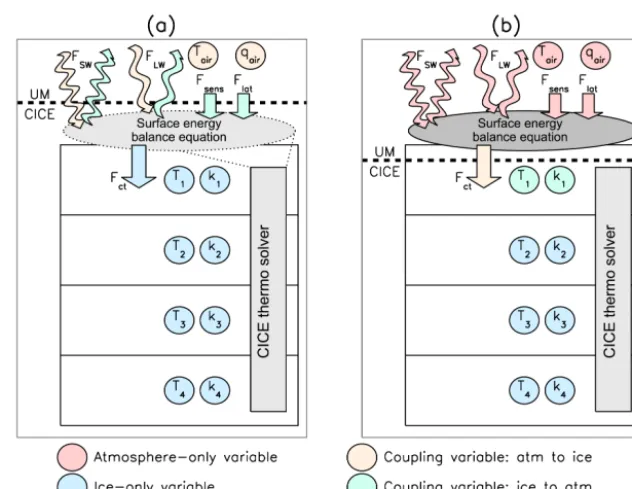
In the standard CICE coupling method (Fig. 1a), the at-mosphere, or surface exchange scheme, calculates fluxes of incoming shortwave and longwave radiation based on the evolving atmospheric state whose lower boundary condition is the ice surface temperature from the previous coupling instant. The atmosphere then averages these over the cou-pling period, and passes them to CICE at the end of that pe-riod. CICE then uses these incoming fluxes throughout the same coupling period in the first row of the tridiagonal ma-trix equation in the row concerning the surface temperature (Eq. 10), each time iterating the solver until convergence is achieved. In the process, CICE computes the remaining surface fluxes (outgoing radiative, turbulent, and conductive fluxes) and hence the net surface flux. This approach is equiv-alent to placing an interface between JULES and CICE im-mediately above the ice surface.
In the alternative JULES coupling method under investi-gation (Fig. 1b), the surface temperature is a prognostic vari-able of the atmosphere or surface exchange model, and is not passed from CICE; instead, the temperature and effec-tive conductivity (the latter defined as 2K1
h1 )of the top ice
Figure 1. Schematics demonstrating (a) the CICE coupling method; (b) the JULES coupling method. In this figureFSW,FLW,Fsens, andFlat
denote fluxes of shortwave radiation, longwave radiation, sensible, and latent heat, respectively;Fct, the conductive flux from the surface to
the ice;Tairandqair, the temperature and humidity of the lowest atmospheric layer; andTjandkj, the temperature and effective conductivity
of ice layerj.
proceeds to solve the tridiagonal matrix occasion in the nor-mal way, except that the top row of the equation is removed; the downwards conductive flux provided by the surface ex-change scheme is then used as forcing for the top ice layer. At the end of the coupling period, the new temperature and effective conductivity of the top ice layer are passed back to the atmosphere. This approach is equivalent to placing an in-terface between JULES and CICE immediately below the ice surface.
It should also be noted that in HadGEM3, fluxes are al-ways passed as gridbox means, to ensure conservation. This point only becomes relevant in 3-D modelling, where sea ice may cover only part of a grid cell; in this case, the relevant flux is multiplied by the grid cell ice concentration before being passed to the coupler for regridding. This is necessary because of the parallel coupling of HadGEM3 (see Sect. 4.4); underlying ice concentration may change during a coupling period, and hence the amount of energy being passed must be correctly represented by multiplying, effectively, by the area over which it is valid.
3 Testing the impact of varying resolution on an idealized solver
3.1 Setup
In this experiment, the penetrating solar radiation term was ignored, and the ice was assumed to be fresh, in order so the
conductivity and specific heat capacity are constant. The ice was assumed to be 1 m thick, and there is no snow cover. The diffusion equation was forced at the top of the ice by a sinusoidally varying heat flux:
Fsfc=ARe(expiωt ) . (12)
There exists an exact analytical solution to the diffusion equation with this surface forcing, for an infinitely deep ice cover (after Best et al., 2005):
T =TB+
A √
ρcωkRe
exp−z
l expi
−
z l +ωt−
π
4
, (13)
whereT →TBasz→ ∞.l= q
2k
ρcωis the e-folding depth. This analytical solution was compared to the solution from the CICE temperature solver under six different conditions, summarized in Table 1. In these experiments, the time step length, coupling period length and vertical resolution were varied, from extremely low values designed to give results as close as possible to ground truth, to higher values considered to be typical of coupled model experiments.
3.2 Results
A. E. West et al.: The location of the thermodynamic atmosphere–ice interface 1129
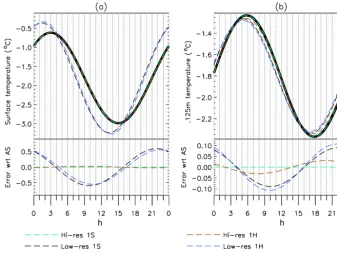
Figure 2. The performance of the CICE temperature solver under varying spatial resolution and time step length, with coupling period 1 h.
Showing (a) surface temperature; (b) temperature at 0.125 m depth.
Table 1. Initial experiments comparing CICE under six different
resolutions.
Experiment Vertical resolution Time step Coupling length period
length
1 (Hi-res 1S) 1 cm (100 layers) 1 s 1 s 2 (Low-res 1S) 25 cm (4 layers) 1 s 1 s 3 (Hi-res 1H) 1 cm (100 layers) 1 h 1 h 4 (Low-res 1H) 25 cm (4 layers) 1 h 1 h 5 (Hi-res 3H) 1 cm (100 layers) 1 h 3 h 6 (Low-res 3H) 25 cm (4 layers) 1 h 3 h
layer temperature in standard CICE, which uses four vertical layers). It is clear that under very high temporal and verti-cal resolution, CICE produces a simulation that is virtually indistinguishable from the analytic solution. As one would expect, when these resolutions are reduced to more realistic levels inaccuracies appear.
When the time step length is increased to 1 h (but the high vertical resolution is maintained), there is a slight increase in the error of the surface temperature simulation, which is still very small in proportion to the cycle amplitude. For the 0.125 m temperature, a small phase lead of around 30 min is introduced, and the amplitude is reduced by a tiny amount (0.02◦C); the diurnal cycle of 0.125 m temperature error has an amplitude of about 0.03◦C.
The effect of decreasing the vertical resolution is more marked. For the surface temperature, we see a large phase lead introduced, of 90 min, but also a marked increase in am-plitude, from 1.2 to 1.5◦C; this results in some comparatively high errors, of up to 0.6◦C. On the other hand, the diurnal cy-cle of 0.125 m temperature is reduced in amplitude slightly, and has a lower phase lead of about 1 h. The errors have mag-nitude of up to 0.09◦C. The contrasting effects of the de-creased vertical resolution on surface and top layer tempera-ture can be understood by considering that the surface tem-perature is forced by the air temtem-perature, and damped by the ice temperature. A top ice layer of thickness 1 cm can warm or cool more easily for a given forcing than a top ice layer of thickness 25 cm; therefore, when the entire top 25 cm of ice has to vary in unison, the amplitude of its cycle is reduced, and its damping effect on the surface temperature is corre-spondingly reduced, which can hence vary more strongly in response to the air temperature forcing.
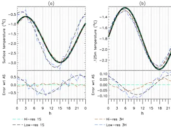
Figure 3. The performance of the CICE temperature solver under varying spatial resolution and time step length, with coupling period 3 h.
Showing (a) surface temperature; (b) temperature at 0.125 m depth.
The error in the four-layer experiment should give cause for concern, as this is a fairly realistic resolution for most implementations of CICE in coupled models. In the next sec-tion, therefore, we compare the simulations at realistic reso-lution, using the two different coupling methods.
4 Comparing the two coupling methods under realistic resolution
4.1 Setup
For this experiment, the solver was run under six different setups. Firstly, two control experiments were undertaken, in which the ice, atmosphere and coupling time steps were each 1 s. In the first control, the ice was given 100 layers, to pro-vide a truth against which to compare subsequent experi-ments; in the second control, the ice was given four layers, to separate the effects of high time step values from the ef-fects of low vertical resolution. The two control experiments were run using the CICE coupling method, with the surface variables calculated by the ice model, but at these time step values the coupling method has negligible impact on the sim-ulation.
The solver was then run with four vertical layers, an ice time step of 1 h, atmosphere time step 20 min, and coupling period of 1 h – fairly realistic values for a coupled model – using the two different coupling methods, CICE and JULES. A further two experiments were then performed, using a
cou-pling period of 3 h, also a common period found in coupled model runs.
The solver was forced with incoming sensible heat flux only, driven by a diurnal cycle of atmospheric surface tem-peratureTatmos=ATexpiωt, with wind speed set to 5 m s−1. For the CICE coupling,Tatmos is averaged over a coupling
period and passed to the ice model, which calculates the in-coming sensible heat flux from this, and uses it as forcing for the temperature solver to calculate internal and surface ice temperatures. For the JULES coupling, a self-contained atmosphere model usesTatmosandT1(top-layer ice
tempera-ture) to implicitly calculate surface fluxes, includingFcondtop,
downwards conductive flux, accumulates and averages this over the coupling period and passes it to the ice model as forcing for the solver.
4.2 Results 4.2.1 1 h coupling
A. E. West et al.: The location of the thermodynamic atmosphere–ice interface 1131
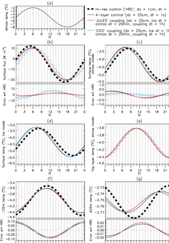
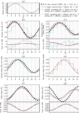
Figure 4. Comparing the two coupling methods, with a 1 h coupling period. Showing (a) atmospheric air temperature (the experiment
forcing); (b) surface flux; (c) surface temperature, as seen by the atmosphere; (d) surface temperature as seen by the ice; (e) 0.125 m ice temperature as seen by the atmosphere; (f) 0.125 m temperature as seen by the ice; (g) 0.625 m temperature.
line). When the CICE coupling method is used, however, there is an additional phase lag and amplitude decrease, and in addition the diurnal cycle becomes more jagged.
Interpreting these results, it is likely that the additional phase lag is a consequence of the atmosphere model see-ing a surface flux calculated in the previous CICE couplsee-ing period, which is itself based on an atmospheric temperature valid for the period before that, up to 2 h previously. With the JULES method, however, the surface flux is able to respond
immediately to the changing atmospheric temperature. There is a corresponding delay in the atmosphere model sensing the damping response of the top layer ice temperature to the changing surface flux. However, the resulting phase lead is tiny in comparison to the phase lag of the CICE method.
tempo-ral resolution makes little difference, causing a tiny phase lag and a slightly less smooth shape compared to the four-layer control. Using the CICE method produces a much more blocky shape, and a substantial phase lag. However, as the four-layer control itself has a phase lead relative to the high-resolution control, the CICE method actually has a more ac-curate phase; the temporal and vertical errors cancel, while the JULES method maintains a phase lead.
How the ice model sees the surface temperature is demon-strated in Fig. 4d. The diurnal cycle is very similar to that of the atmosphere model surface temperature for the two con-trol runs, due to their low time step length. The ice model does not have knowledge of the surface temperature in the JULES coupling method and this line is not plotted. The sur-face temperature simulation in the CICE method is very sim-ilar to the control; the phase lag experienced by the atmo-sphere model is due to the coupling delay only.
Conversely, Fig. 4e demonstrates how the atmosphere model sees the top layer temperature, in the four-layer con-trol and in the JULES coupling method (as in the CICE method, the atmosphere has no knowledge of this variable). There is a slight phase lag relative to the control, and as-sociated jaggedness of the diurnal cycle, owing to the need to hold the temperature constant over each coupling period, rather than update it every atmospheric time step.
The lower panels (Fig. 4f and g) compare the internal ice temperatures at 0.125 m (top layer) and 0.625 m (third layer) depth in the four experiments. For both variables, the de-crease in vertical resolution is characterized by a dede-crease in amplitude and a phase lead which are both more severe in the deeper variable. The decrease in time step length pro-duces additional amplitude decrease and phase lead which are very similar in the two coupling methods. It is interesting to note that the errors are marginally smaller for the JULES method. This is likely due to the fact that in the JULES method, changes inTatmoscan propagate quickly downwards
to changes tofsurfon the 20 min atmospheric time step, the
main bottleneck occurring in the coupling, as fsurf forces
changes inT1on the slower 1 h coupling period. In contrast,
in the CICE method, each link in the chain – fromTair, to
Tsfc andfcondtop, toT1 – must communicate on a slow 1 h
time step. In consequence, the JULES method simulation is slightly closer to that of the four-layer control.
4.2.2 3 h coupling
The results of the experiments when 3 h coupling is used are shown in Fig. 5. For the surface flux (Fig. 5b), again, de-creasing temporal resolution is identified with a small phase lag and amplitude decrease in the JULES method; the simu-lation is very similar to that with the 1 h coupling period, al-though slightly less smooth. For the CICE method, however, the phase lag and amplitude decrease are greatly magnified; the peak of the diurnal cycle occurs 2–3 h too late, and the cycle has a very discontinuous shape.
Considering the surface temperature (Fig. 5c), the JULES method again produces a simulation with a 3 h coupling pe-riod which is quite similar to that with the 1 h pepe-riod, though less smooth. Again, the effect of the CICE method is to pro-duce a phase lag. Whereas in the 1 h coupling period case, however, this phase lag almost exactly cancelled the lead of the increased vertical resolution, in the 3 h case the lead is much greater, and the absolute phase error of the method is actually greater than that of the JULES method, in an inter-esting demonstration of the dangers of cancelling errors.
When considering the ice variables (Fig. 5f and g) there are again few clear differences between the simulations, but again the error is marginally smaller for the JULES method than for the CICE method. Again this is likely related to the chain by which changes propagate fromTatmos, viaTsfc and
fsurf, toT1. The JULES method involves a fast link, on the
20 min atmospheric time step, fromTatmostoTsfc andfsurf,
and a very slow link, on the 3 h coupling time step, fromfsurf
toT1. By contrast, the CICE method involves a very slow
link, on the 3 h coupling time step, fromTatmos toTsfc and
fsurf, and a slow link, on the 1 h CICE time step, fromTsfc
toT1. While the rate of propagation is dominated for both
methods by the 3 h coupling bottleneck, changes inTatmosare
still able to propagate slightly more quickly with the JULES method.
In summary, the deterioration in simulation of the atmo-spheric variables that is associated with decreased temporal resolution is significantly reduced by using the JULES cou-pling method. There is also a small improvement in the sim-ulation of the ice variables, although this is very marginal. 4.3 Varying the parameters of the experiments
To gain some idea of the generality of the results, the pa-rameters of the experiment were varied. Firstly, the coupling methods were tested with an 11 cm snow layer present above the ice. Secondly, they were tested without a snow layer, but with the wind speed increased from 5 to 20 m s−1, to examine the impact of strengthening the coupling between the forcing air temperature and the surface.
The results are presented in Fig. 6a–f, in which for each additional experiment, and for the original experiment, the surface flux and the top layer temperature are plotted. (For the snow layer experiment, the top layer temperature corre-sponds to the snow layer temperature; for the other exper-iments, to the top ice layer temperature.) For clarity, only the two control experiments and the two 3 h coupling exper-iments are shown.
A. E. West et al.: The location of the thermodynamic atmosphere–ice interface 1133
Figure 5. Comparing the two coupling methods, with a 3 h coupling period. Showing (a) atmospheric air temperature (the experiment
forcing); (b) surface flux; (c) surface temperature, as seen by the atmosphere; (d) surface temperature as seen by the ice; (e) 0.125 m ice temperature as seen by the atmosphere; (f) 0.125 m temperature as seen by the ice; (g) 0.625 m temperature.
layer temperature, and thus allowing the surface flux to over-shoot. However, the errors are still far smaller than those of the CICE method. The snow layer temperature (Fig. 6b, d) has a much larger diurnal cycle than the top ice layer tem-perature in the original experiment, due to its much lower heat capacity. Relative to the four-layer control, the JULES method overestimates the amplitude, while the CICE method underestimates the amplitude, precisely as is the case for the surface flux.
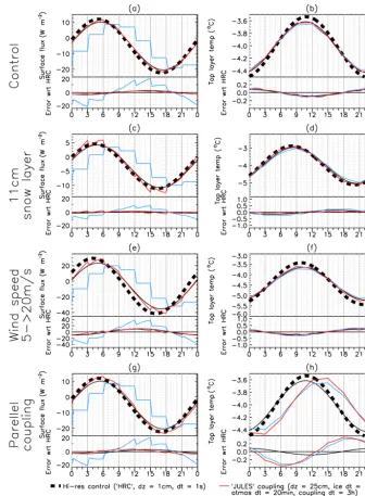
Figure 6. Demonstrating the performance of the two coupling methods when the parameters of the experiment are varied. Showing surface
flux (left) and top-layer temperature (right) for (a, b) original experiment; (c, d) an experiment in which an 11 cm snow layer was present on the ice; (e, f) an experiment in which wind speed was increased from 5 to 20 m s−1; (g, h) an experiment in which parallel, rather than serial, coupling was employed. For the snow layer experiment, the top-layer temperature represents the temperature of the snow layer; for all others, it represents the temperature of the top ice layer.
speed, and is therefore 4 times greater in this experiment; the overall surface flux amplitude, although larger than in the 5 m s−1 experiment, does not increase in direct proportion. Hence the overshoot is higher in proportion here. However, the JULES method errors are still considerably lower than those of the CICE method. For the top layer ice tempera-ture (Fig. 6f), both methods produce simulations very close to those of the four-layer control.
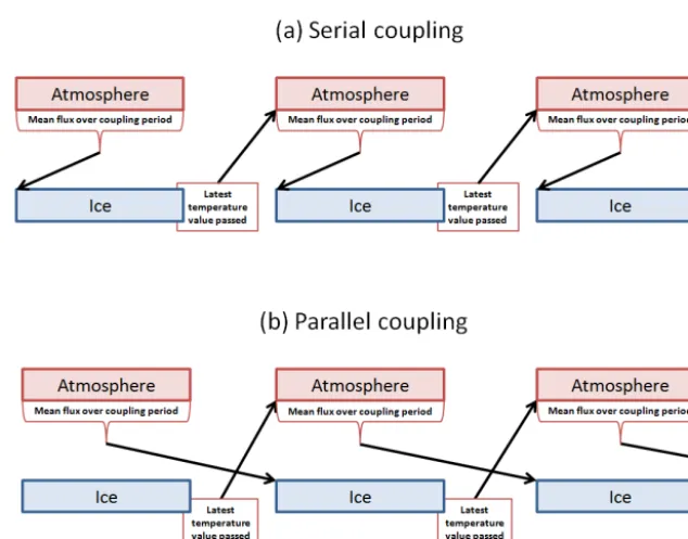
4.4 Serial versus parallel coupling
alter-A. E. West et al.: The location of the thermodynamic atmosphere–ice interface 1135
Figure 7. Schematic demonstrating the (a) serial and (b) parallel coupling frameworks, as described in Sect. 4.4.
native parallel method, in which atmosphere and ice models are run concurrently. This entails that the atmosphere-to-ice forcing flux is used instead as forcing for the ice during the coupling period after that in which it was calculated. The se-rial and parallel frameworks are demonstrated schematically in Fig. 7.
The parallel method can be more computationally effi-cient, but is less accurate (as is demonstrated below). The tests of Sect. 4.1–4.3 were carried out below using the series method, despite HadGEM3 using the parallel method, in or-der to eliminate the additional source of inaccuracy caused by parallel coupling and therefore enable the results to be more relevant to the wider community. However, it is also useful to compare the relative performance of the CICE and JULES methods under parallel conditions. The tests were therefore carried out again, with the 1-D solver edited to mimic a parallel system, rather than a serial one.
The results are shown in Fig. 6a–b (serial coupling) and Fig. 6g–h (parallel coupling). As seen in the sensitivity ex-periments of Sect. 4.3, the JULES method displays a dete-rioration in the surface flux simulation relative to the con-trol (series coupling), shown in Fig. 6g, with the surface flux overshoot again enhanced, and the amplitude increased ac-cordingly, a result of the extra 3 h of delay in the atmosphere receiving a damping response from the top layer temper-ature to the original overshoot. The reason that the CICE method does not display a similar deterioration is that for this method, one of the variables immediately adjacent to the interface (the air temperature), is not free to vary in this ex-periment, but prescribed, and therefore the atmosphere pays no penalty for the delay in receiving the forcing from
be-low – a situation which would not occur in a fully cou-pled model. The 3 h lag introduced to the top layer temper-ature simulation (Fig. 6h) is noticeable in both the JULES and CICE methods, and incidentally demonstrates, indepen-dently of this study, the drawbacks of using parallel coupling as opposed to serial. It should be pointed out however that this drawback is much reduced when 1 h coupling is used; also, that despite the deterioration, the surface flux errors for the JULES method are still substantially lower than those of the CICE method.
5 Discussion and conclusions
What is the reason for the improved simulation obtained by simulating surface variables within the atmosphere model, rather than the ice model? The root cause is probably that in the experiments, as is usually the case in coupled models and in the real world, the principal thermodynamic forcing on the surface, and the ice, comes from above rather than below. Air temperature and radiation conditions usually change more rapidly than do properties of the underlying ocean, and of the sub-surface ice. Therefore it is not surprising that an im-proved simulation is obtained by placing a higher proportion of the ice-surface system within the atmosphere model, from which the forcing comes. With a thin snow cover present, or with increased wind speed, the improvements offered by the JULES method grow slightly less. The reason is likely that both modifications have the effect, for the JULES method, of increasing the magnitude of the surface flux response during each coupling period relative to the surface flux amplitude, thus allowing the overestimation of the amplitude to be wors-ened. There is no corresponding deterioration for the CICE method, as the surface flux does not change during the cou-pling period. However, the JULES method still produces sub-stantially lower surface flux errors. It can be concluded that although the top layer temperature simulation is not system-atically better in either method, the JULES method produces a better surface flux simulation under most circumstances.
At first sight, this conclusion appears to disagree with the statement in the introduction to Sect. 2 of the CICE docu-mentation (Hunke et al., 2013) that “accuracy may be signif-icantly reduced” by solving for surface temperature in the at-mosphere model. However, this statement relates specifically to the hypothetical necessity of artificially reducing effective conductivity to ensure stability in such a situation, rather than the inherent accuracy of the coupling method. In practice, we have found that reducing effective conductivity is not neces-sary (see Appendix A).
This prompts the following question: how realistic were the conditions under which the one-dimensional experiments were held, and to what degree would this improvement carry across to the simulation of ice and atmospheric variables in a non-idealized setting? Clearly the best way to answer this question would be to test two coupled models, one us-ing each method. However, the differences between the two setups involve substantial structural changes to all compo-nents of the HadGEM3 model, and this option was deemed impractical. Following the results of these experiments, the JULES coupling method is being implemented in the Met Office HadGEM3-GC3 coupled model for use with CICE’s capability for multilayer thermodynamics, and when this be-comes operational there will be an opportunity to compare the simulation of processes over sea ice to other fully pled models which use CICE with the standard CICE cou-pling method. It is nevertheless possible to use the insight provided by the idealized experiments to gain some idea of the likely effects of the different coupling methods in a 3-D simulation.
The principal effect of the CICE coupling, as opposed to the JULES coupling, is to damp and delay the response of the surface flux (equal in these experiments to the sensible heat flux) to changes in surface air temperature. These changes are applied in the experiments as variations of around 5◦C in the course of about 12 h. Variations in air temperature of this rate and magnitude are common in the Arctic Ocean, although often they occur in response to changes in cloud cover, or the passage of frontal boundaries, rather than to the diurnal cycle (e.g. Persson et al., 2002). Nevertheless, the implication of the 1-D experiments is that a model using the CICE coupling method will simulate a surface flux response that is overly delayed and damped, relative to a model using the JULES coupling. In effect, the coupling between the atmosphere and the underlying sea ice is weaker, and the atmosphere is likely to behave more like an isolated system.
The effects of this would be complex. A mild air mass moving over cold sea ice tends to be diabatically cooled at the surface via the surface flux response, while the opposite will occur when a cold air mass moves over less cold sea ice. A delayed and damped surface flux response would tend to reduce the rate of modification of air masses, allowing them to retain characteristics for longer. A similar effect would be likely to be seen in the event of air temperatures responding to changes in radiative forcing due to cloud cover. Normally, the response of surface flux would likely be to moderate di-abatic heating or cooling of air masses due to these radiative effects, by transferring some of this heating or cooling into the sea ice; a delayed, damped response would hinder this modification. In this way, it is possible that anomalous char-acteristics of neighbouring air masses would become more exaggerated, relative to the real world, when using the CICE coupling method, with unpredictable consequences for at-mospheric dynamics. The perturbed parameter experiments demonstrate that under very windy, stormy conditions, the reverse effect might be seen; the surface flux could respond too quickly, and too strongly, thus allowing air mass modifi-cation to take place too quickly.
It is seen in Sect. 4 that the choice of coupling method has little direct impact on the internal sea ice simulation. How-ever, the sea ice simulation will be strongly affected through the atmospheric response described above, whose dynamics will affect advection of warm and cold air over the ice, as well as advection of the ice itself. As the JULES coupling method produces a more realistic surface flux response to changes in air temperature, it appears clear that, all other fac-tors being equal, this coupling method would simulate a more accurate evolution of atmosphere and sea ice.
sug-A. E. West et al.: The location of the thermodynamic atmosphere–ice interface 1137 gests that the implementation of variably spaced layers, with
higher resolution near the top of the ice, would be a logical objective to pursue subsequently, to further improve surface flux simulation.
The main focus of this study has been the accuracy of the two coupling methods; a separate question is their sta-bility. The CICE method of coupling is known to have ma-jor problems of instability arising from the explicit inter-face in the surinter-face exchange, an area where processes oc-cur relatively quickly (e.g. Best et al., 2004). However, the JULES method has its own explicit interface, below the ice surface, and is therefore also likely to become unstable un-der certain conditions. A detailed analysis of the stability of the JULES method in the one-dimensional case is described in Appendix A. The principal factors affecting stability are found to be ice thickness and wind speed; a prediction from this analysis is that setting a minimum ice thickness of 30 cm
in a coupled model is sufficient to avoid instability in all situ-ations. In practice, however, in test runs of the coupled model a minimum ice thickness of 20 cm has been found to be suf-ficient to avoid instability. This is probably because in the fully coupled model, other negative feedbacks are at work in the atmosphere that act to damp oscillations caused by the explicit coupling, and prevent instability.
It is planned to follow this paper with a study examining the simulation of sea ice in HadGEM3 resulting from the im-plementation of multilayer sea ice, using the JULES coupling method.
Code availability
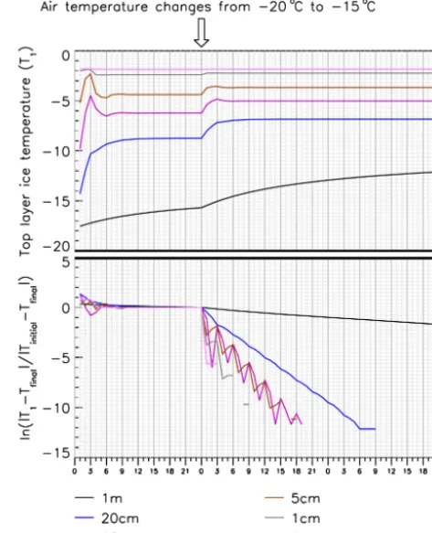
Appendix A: Stability of the JULES method of coupling In this section, the one-dimensional model is used to investi-gate the conditions under which the solver becomes unstable, prior to its implementation in the Met Office coupled model. In the stability experiment, the model was run for 5 days; for the first day, the atmospheric temperature was held con-stant at−20◦C, but at the beginning of the second day, the atmospheric temperature was abruptly changed to −15◦C; the solver was judged to be stable or unstable according to whether the variables converged to a new solution, and the nature of the convergence was examined. The test was per-formed under typical modelling conditions of four ice layers, ice time step 1 h, atmospheric time step 20 min, and of cou-pling period length 3 h. The initial parameter that was varied was the ice thickness; the test was performed for six different thicknesses of ice: 1 m, 20 cm, 10 cm, 5 cm, 1 cm, and 1 mm. In each case, the top layer ice temperature converged to a new solution, the convergence tending to be most rapid for the thinnest ice (Fig. A1).
From this it appears that under normal modelling condi-tions, the JULES coupling method is not inherently unsta-ble to sudden perturbations, and tends to be more, rather than less, stable for thin ice. This is perhaps surprising, as it would be thought that thin ice would tend to react more sen-sitively to perturbations in conductive flux, given its lower thermal inertia. However, counteracting this is the higher ef-fective conductivity of thin ice, meaning that perturbations in top conductive flux will tend to propagate more rapidly through the ice during a coupling period, reducing the result-ing change in top layer ice temperature. It also means that as ice thins, the response of the conductive flux comes to dom-inate the surface energy balance, effectively locking surface temperature to top layer ice temperature, and reducing varia-tion in conductive flux.
To examine the reasons for the stability more carefully, we derive theoretical limits on perturbations to top layer tem-perature and conductive flux. Given an equilibrium solution to the coupled system Feq, T1_eq, Tsfc_eq
, and perturbations around this solutionF,ˆ Tˆ1,Tˆsfc
, it can be shown from the surface energy balance equation that the perturbation con-ductive flux produced by the atmosphere is constrained by the perturbation top layer ice temperature in the following way: ˆ F ≤
keffOFE
keff+OFE
· ˆ T1 , (A1)
wherekeff=2k1/h1is the effective conductivity of the top
layer and OFE= ˙fsens Tsfc_eq+ ˙flat Tsfc_eq+ ˙frad Tsfc_eq
represents the total rate of change of the surface radiative, sensible, and latent heat fluxes with respect to surface tem-perature at Tsfc=Tsfc_eq, and tends to reach its highest
val-ues under very windy, stormy conditions. It can be seen that the controlling constant here tends to the finite limit OFE as
h1→0.
Figure A1. Showing the evolution of top layer ice
tempera-ture following a sudden change in air temperatempera-ture, under the JULES coupling method. The lower panel shows the evolution of ln |T1−Tfinal|
|Tinitial−Tfinal|
to allow easy comparison of the rates of conver-gence for differing ice thicknesses, whereT1,Tfinal, andTinitial
re-spectively refer to the evolving top layer ice temperature, the value of top layer ice temperature after 3 days, and the value at 1 day, at the time of the perturbation. The graph disappears when the differ-ence falls below minimum precision
Meanwhile, in the ice thermodynamic solver, energy bal-ance considerations provide a constraint on the magnitude of the change inTˆ1during a coupling period:
|1T1| ≤
tc
cpρiceh1
|F|, (A2)
wheretc,cp,ρice, andh1represent coupling period length,
ice heat capacity, ice density and top layer ice thickness, respectively. This, together with Eq. (A1), prevents insta-bility for tcOFE
h1 < cpρice. The system is therefore stable for h1>5 cm (equivalently total ice thickness<20 cm) in all but
the most extreme atmospheric conditions, and forh1>10 cm
(equivalently ice thickness<40 cm) under all realistic atmo-spheric conditions.
be-A. E. West et al.: The location of the thermodynamic atmosphere–ice interface 1139
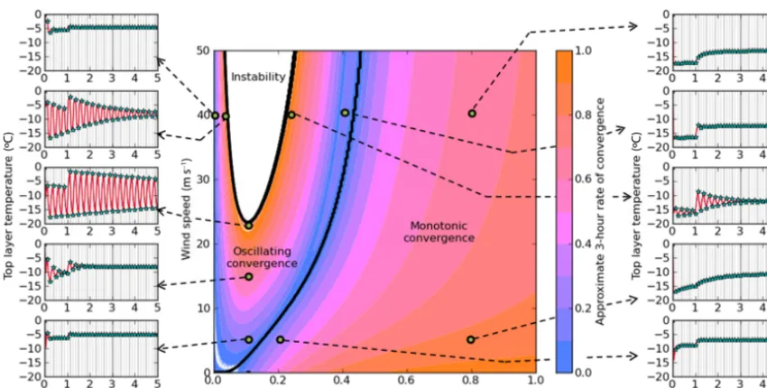
Figure A2. Map of stability of the coupled ice and surface solvers, as ice thickness and wind speed are varied, with a 3 h coupling period.
Speed of convergence is indicated in colour, where blue is rapid convergence, red is slow convergence. Regions of 3 h monotonic convergence, 3 h oscillating convergence and instability are indicated. Time series of top layer ice temperature are shown for 10 representative points of the variable space.
comes negligible for ice of layer thickness under about 2 cm, causing the dominant balance in the equation to be between top conductive flux and conduction with the layer below. In this situation, given a top conductive forcing, the ice tem-peratures will converge very quickly to a linear temperature profile with uniform conductive flux, meaning that
ˆ T1
=
h1
2k1
ˆ F1
. (A3)
Combined with Eq. (A1), this prevents instability com-pletely.
In summary, Eqs. (A1), (A2), and (A3) show that instabil-ity cannot occur in the limit of very thick ice (when thermal inertia dominates), due to a highly damped response of top layer temperature to perturbations of conductive flux, and also cannot occur in the limit of very thin ice (when con-duction to the ocean dominates), due to the surface tempera-ture becoming virtually locked to top layer ice temperatempera-ture, perturbations in conductive flux becoming correspondingly small (i.e. whenkeffOFE), and these perturbations very
easily propagating through the ice to the ocean. It is notice-able that in Fig. A1, the least stnotice-able solutions appear to occur for intermediate ice thicknesses (5, 10 cm), when neither con-duction nor thermal inertia dominates, but the overlap in the two conditions is nevertheless sufficient to allow a relatively rapid convergence.
The question arises as to whether the solver would con-tinue to converge for all ice thicknesses if any of the param-eters in Eqs. (A1), (A2), or (A3) altered. Paramparam-eterscp,ρice,
andtc cp are assumed to be at the lower, lower, and upper
Figure A3. Map of stability of the coupled ice and surface solvers,
as ice thickness and wind speed are varied, with a 1 h coupling pe-riod.
depressions, however, wind speeds can reach much higher values.
The perturbation experiment was repeated, but this time two parameters were varied: ice thickness from 1 mm to 1 m, and wind speed from 0 to 50 m s−1, the upper limit roughly representing the very highest wind speeds possible during ex-tratropical storms. The results are shown in Fig. A2. It is seen that the solver is no longer unconditionally stable, with insta-bility setting in at a wind speed of around 23 m s−1, at first for a narrow band of ice thicknesses close to 10 cm, a band which steadily widens as wind speed increases. At all wind speeds the solver remains stable in the limit of thin ice. How-ever, at the upper limit of wind speed, the solver is unstable for ice thicknesses of between roughly 4 and 25 cm.
This result holds fortc=3 h, buttc=1 h is also a fairly
widely used coupling period, and is likely to become more so as computing power increases. The experiment was re-peated fortc=1 h (Fig. A3). In this case, the solver is stable
for all ice thicknesses and wind speeds, although at the up-per limit of wind speed, convergence is extremely slow for ice thicknesses of around 7 cm. (Clearly the second region of slow convergence, to the right of the figure, is not a con-cern, as this is caused by higher thermal inertia of thick ice, is entirely physically realistic, and will not lead to instability.)
A. E. West et al.: The location of the thermodynamic atmosphere–ice interface 1141 The Supplement related to this article is available online
at doi:10.5194/gmd-9-1125-2016-supplement.
Author contributions. The JULES method of coupling was
origi-nally devised by Martin Best. The one-dimensional experiments of Sects. 3 and 4.1 were designed and carried out by Alison McLaren. The perturbation experiments of Sect. 4.3, the parallel coupling ex-periments of Sect. 4.4, and the stability exex-periments of the Ap-pendix were designed and carried out by Alex West. All results were plotted and analysed by Alex West with advice and assistance from Alison McLaren, Martin Best, and Helene Hewitt. The paper was written in its final form by Alex West with input from all three con-tributing authors.
Acknowledgements. The authors thank Ann Keen and Ed Blockley
for help and advice prior to submission, and also thank Dirk Notz and Anton Beljaars for their insightful reviews.
This study was supported by the Joint UK DECC/Defra Met Office Hadley Centre Climate Programme (GA01101).
Edited by: D. Goldberg
References
Best, M. J., Beljaars, A., Polcher, J., and Viterbo, P.: A Proposed Structure for Coupling Tiled Surfaces with the Planetary Bound-ary Layer, J. Hydrometerorol., 5, 1271–1278, doi:10.1175/JHM-382.1, 2004.
Best, M. J., Cox, P. M., and Warrilow, D. M.: Determining the opti-mal soil temperature scheme for atmospheric modelling applica-tions, Bound. Lay. Meteorol., 114, 111–142, 2005.
Best, M. J., Pryor, M., Clark, D. B., Rooney, G. G., Essery, R .L. H., Ménard, C. B., Edwards, J. M., Hendry, M. A., Porson, A., Gedney, N., Mercado, L. M., Sitch, S., Blyth, E., Boucher, O., Cox, P. M., Grimmond, C. S. B., and Harding, R. J.: The Joint UK Land Environment Simulator (JULES), model description – Part 1: Energy and water fluxes, Geosci. Model Dev., 4, 677–699, doi:10.5194/gmd-4-677-2011, 2011.
Bitz, C. M. and Lipscomb, W. H.: An energy-conserving thermo-dynamic model of sea ice, J. Geophys. Res., 104, 15669–15677, 1999.
Gordon, C., Cooper, C., Senior, C. A., Banks, H., Gregory, J. M., Johns, T. C., Mitchell, J. F. B., and Wood, R. A.: The simulation of SST, sea ice extents and ocean heat transports in a version of the Hadley Centre coupled model without flux adjustments, Clim. Dynam., 16, 147–168, doi:10.1007/s003820050010, 2000.
Hewitt, H. T., Copsey, D., Culverwell, I. D., Harris, C. M., Hill, R. S. R., Keen, A. B., McLaren, A. J., and Hunke, E. C.: Design and implementation of the infrastructure of HadGEM3: the next-generation Met Office climate modelling system, Geosci. Model Dev., 4, 223–253, doi:10.5194/gmd-4-223-2011, 2011.
Hunke, E. C., Lipscomb, W. H., Turner, A. K., Jeffery, N., and Elliott, S.: CICE: the Los Alamos Sea Ice Model, Documen-tation and Software, Version 5.0, Los Alamos National Lab-oratory Tech. Rep. LA-CC-06-012, Los Alamos, New Mex-ico, available at: http://oceans11.lanl.gov/trac/CICE/attachment/ wiki/WikiStart/cicedoc.pdf?format=raw (last access: 27 October 2015), 2013.
Johns, T. C., Durman, C. F., Banks, H. T., Roberts, M. J., McLaren, A. J., Ridley, J. K., Senior, C. A., Williams, K. D., Jones, A., Rickard, G. J., C. S., Ingram, W. J., Crucifix, M., Sexton, D. M. H., Joshi, M. M., Dong, B.-W., Spencer, H., Hill, R. S. R., Gre-gory, J. M., Keen, A. B., Pardaens, A. K., Lowe, J. A., Bodas-Salcedo, A., Stark, S., and Searl, Y.: The New Hadley Centre Cli-mate Model (HadGEM1): Evaluation of Coupled Simulations, J. Climate, 19, 1327–1353, doi:10.1175/JCLI3712.1, 2006. Maykut, G. A. and Untersteiner, N.: Some Results from a
Time-Dependent Thermo-dynamic Model of Sea Ice, J. Geophys. Res., 7, 1550–1575, 1971.
Ono, N.: Specific heat and fusion of sea ice, Physics of Snow and Ice, 1, 599–610, 1967.
Persson, P. O. G., Fairall, C. W., Andreas, E. L., Guest, P. S., and Perovich, D. K.: Measurements near the Atmospheric Surface Flux Group tower at SHEBA: Near-surface condi-tions and surface energy budget, J. Geophys. Res., 107, 8045, doi:10.1029/2000JC000705, 2002.
Semtner, A. J.: A Model for the Thermodynamic Growth of Sea Ice in Numerical Investigations of Climate, J. Phys. Oceanogr., 6, 379–389, 1975.
Untersteiner, N.: Calculations of temperature regime and heat bud-get of sea ice in the Central Arctic, J. Geophys. Res., 69, 755– 4766, 1964.