https://doi.org/10.5194/gmd-11-2273-2018 © Author(s) 2018. This work is distributed under the Creative Commons Attribution 4.0 License.
FAIR v1.3: a simple emissions-based impulse response and
carbon cycle model
Christopher J. Smith1, Piers M. Forster1, Myles Allen2, Nicholas Leach2, Richard J. Millar3,4, Giovanni A. Passerello1, and Leighton A. Regayre1
1School of Earth and Environment, University of Leeds, Leeds, UK 2Atmospheric Physics Department, University of Oxford, Oxford, UK
3College of Engineering, Mathematics and Physical Sciences, University of Exeter, Exeter, UK 4Environmental Change Institute, University of Oxford, Oxford, UK
Correspondence:Christopher J. Smith ([email protected]) Received: 25 October 2017 – Discussion started: 7 December 2017 Revised: 8 May 2018 – Accepted: 11 May 2018 – Published: 18 June 2018
Abstract.Simple climate models can be valuable if they are able to replicate aspects of complex fully coupled earth sys-tem models. Larger ensembles can be produced, enabling a probabilistic view of future climate change. A simple emissions-based climate model, FAIR, is presented, which calculates atmospheric concentrations of greenhouse gases and effective radiative forcing (ERF) from greenhouse gases, aerosols, ozone and other agents. Model runs are constrained to observed temperature change from 1880 to 2016 and pro-duce a range of future projections under the Representative Concentration Pathway (RCP) scenarios. The constrained es-timates of equilibrium climate sensitivity (ECS), transient climate response (TCR) and transient climate response to cu-mulative CO2emissions (TCRE) are 2.86 (2.01 to 4.22) K, 1.53 (1.05 to 2.41) K and 1.40 (0.96 to 2.23) K (1000 GtC)−1 (median and 5–95 % credible intervals). These are in good agreement with the likely Intergovernmental Panel on Cli-mate Change (IPCC) Fifth Assessment Report (AR5) range, noting that AR5 estimates were derived from a combina-tion of climate models, observacombina-tions and expert judgement. The ranges of future projections of temperature and ranges of estimates of ECS, TCR and TCRE are somewhat sensi-tive to the prior distributions of ECS/TCR parameters but less sensitive to the ERF from a doubling of CO2or the ob-servational temperature dataset used to constrain the ensem-ble. Taking these sensitivities into account, there is no evi-dence to suggest that the median and credible range of ob-servationally constrained TCR or ECS differ from climate model-derived estimates. The range of temperature
projec-tions under RCP8.5 for 2081–2100 in the constrained FAIR model ensemble is lower than the emissions-based estimate reported in AR5 by half a degree, owing to differences in forcing assumptions and ECS/TCR distributions.
1 Introduction
Earth system models in CMIP5 all show a positive car-bon cycle feedback, meaning that as surface temperature increases, land and ocean carbon sinks become less effec-tive at absorbing CO2 and a larger proportion of any fur-ther emitted carbon will remain in the atmosphere (Friedling-stein, 2015). The various feedback strengths are nevertheless model dependent (Friedlingstein et al., 2006). While CO2is the most important climate forcer, individual models may also differ in their responses to non-CO2 emissions. These emissions can also introduce uncertainty that is not captured in concentration-driven or CO2-only driven model experi-ments (Matthews and Zickfeld, 2012; Tachiiri et al., 2015; Gasser et al., 2017). As non-CO2forcing impacts tempera-ture, which affects the efficiency of carbon sinks, non-CO2 forcing agents themselves influence the carbon cycle (Mac-Dougall et al., 2015; Tokarska et al., 2018).
Simple models can be used to emulate radiative forc-ing and temperature responses to emissions and atmospheric concentrations and can be tuned to replicate the behaviour of individual climate and earth system models (Meinshausen et al., 2011a; Good et al., 2011, 2013; Geoffroy et al., 2013). A simple emulation of the carbon cycle of full- and intermediate-complexity earth system models was developed by Joos et al. (2013) and used in the IPCC Fifth Assessment Report (AR5) for the purposes of calculating global warming potentials. The model was developed for a 100 GtC pulse against a background CO2concentration of 389 ppm. Millar et al. (2017) showed that this model does not sufficiently cap-ture the time-evolving dependency of carbon sinks against different background conditions. They introduced the Finite Amplitude Impulse Response (FAIR) model (version 1.0) that tracks the time-integrated airborne fraction of carbon and uses this to determine the efficiency of carbon sinks, in turn calculating atmospheric CO2 concentrations, radiative forc-ing and temperature change.
FAIR v1.0 is well-calibrated to the temperature and car-bon cycle response of earth system models. FAIR v1.3 is extended to calculate non-CO2 greenhouse gas concentra-tions from emissions, aerosol forcing from aerosol precursor emissions, tropospheric and stratospheric ozone forcing from the emissions of precursors, and forcings from black carbon on snow, stratospheric methane oxidation to water vapour, contrails and land use change. Forcings from volcanic erup-tions and solar irradiance fluctuaerup-tions are supplied externally. These forcings are then converted to a temperature change, taking into account the different thermal responses of the ocean mixed layer and deep ocean.
The model philosophy in FAIR is to represent these pro-cesses as simply as possible and to be able to emulate the his-torical effective radiative forcing (ERF) time series in AR5 given input emissions. FAIR is written in Python and is open source. The extension to non-CO2 emissions makes FAIR v1.3 applicable for assessing scenarios with a broad range of emissions pathways.
This paper introduces the FAIR model in Sect. 2, includ-ing the key changes from versions 1.0 to 1.3. Section 3 then discusses the generation of a large ensemble of input param-eters to the FAIR model which is run and results described in Sect. 4. A sensitivity analysis to some of the key inputs to the large ensemble is given in Sect. 5. Section 6 provides a summary.
2 Development of FAIR v1.3 and differences to v1.0 FAIR v1.3 takes emissions of greenhouse gases and short-lived climate forcers as its main input. This is an array of size (number of years×40) (see Table 1) and is based on the order provided in the Representative Concentration Path-way (RCP) emissions datasets (Meinshausen et al., 2011b). Additional options that can be specified by the user include the treatment of aviation contrail and land use forcing, the fraction of total methane attributable to fossil fuels, natural emissions of CH4and N2O, and natural forcing from solar variability and volcanoes. The atmospheric concentrations of greenhouse gases are calculated from new emissions minus the decay of the current atmospheric burden, which is deter-mined by the atmospheric lifetime of each gas, and output is produced as a (years×31) array (Table 2). For CO2, at-mospheric concentrations are calculated from a simple rep-resentation of the carbon cycle which includes temperature and saturation dependency of land and ocean sinks. The cal-culated CO2concentrations at each timestep also include a proportion of methane oxidised to CO2. This is on the as-sumption of a mole of oxidised methane from fossil sources is not also counted as a mole of CO2 when reported in national emissions inventories (Gillenwater, 2008; Boucher et al., 2009).
The effective radiative forcing (ERF) from 13 different forcing agents (Table 3) is determined from the concentra-tions of each greenhouse gas, plus emissions of short-lived climate forcers and natural forcing, and is output from the model as a (years×13) array. From the ERF, temperature change is calculated. The change in temperature feeds back into the carbon cycle, which impacts the atmospheric life-time of carbon dioxide. A flow diagram outlining the key processes is provided in Fig. 1. It is also possible to run FAIR using only CO2emissions as inputs or purely in forcing-only mode, where a time series of non-CO2or total forcing can be optionally specified rather than calculated from emissions. 2.1 Greenhouse gases: emissions to concentrations 2.1.1 Carbon dioxide and carbon cycle
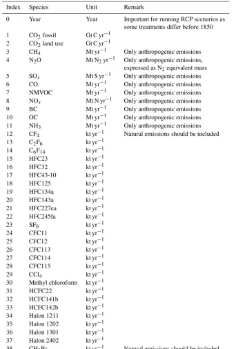
Table 1.Emissions time series input used in FAIR, based on the RCP emissions datasets in Meinshausen et al. (2011b).
Index Species Unit Remark
0 Year Year Important for running RCP scenarios as some treatments differ before 1850 1 CO2fossil Gt C yr−1
2 CO2land use Gt C yr−1
3 CH4 Mt yr−1 Only anthropogenic emissions 4 N2O Mt N2yr−1 Only anthropogenic emissions,
expressed as N2equivalent mass 5 SOx Mt S yr−1 Only anthropogenic emissions 6 CO Mt yr−1 Only anthropogenic emissions 7 NMVOC Mt yr−1 Only anthropogenic emissions 8 NOx Mt N yr−1 Only anthropogenic emissions 9 BC Mt yr−1 Only anthropogenic emissions 10 OC Mt yr−1 Only anthropogenic emissions 11 NH3 Mt yr−1 Only anthropogenic emissions 12 CF4 kt yr−1 Natural emissions should be included 13 C2F6 kt yr−1
14 C6F14 kt yr−1 15 HFC23 kt yr−1 16 HFC32 kt yr−1 17 HFC43-10 kt yr−1 18 HFC125 kt yr−1 19 HFC134a kt yr−1 20 HFC143a kt yr−1 21 HFC227ea kt yr−1 22 HFC245fa kt yr−1 23 SF6 kt yr−1 24 CFC11 kt yr−1 25 CFC12 kt yr−1 26 CFC113 kt yr−1 27 CFC114 kt yr−1 28 CFC115 kt yr−1 29 CCl4 kt yr−1 30 Methyl chloroform kt yr−1 31 HCFC22 kt yr−1 32 HCFC141b kt yr−1 33 HCFC142b kt yr−1 34 Halon 1211 kt yr−1 35 Halon 1202 kt yr−1 36 Halon 1301 kt yr−1 37 Halon 2402 kt yr−1
38 CH3Br kt yr−1 Natural emissions should be included 39 CH3Cl kt yr−1 Natural emissions should be included
differing timescales of carbon uptake by geological processes (τ0), the deep ocean (τ1), the biosphere (τ2) and the ocean mixed layer (τ3). The atmospheric molar mixing ratio of CO2 and its relationship to each box is
CCO2=CCO2,pi+ 3 X
i=0 Ri
Ma wCO2
wa
, (1)
withCCO2,piequal to 278 ppm and the subscript pi
represent-ing a pre-industrial state.Ma=5.1352×10¹⁸kg is the dry mass of the atmosphere, andwCO2 andwaare the molecular
weights of CO2and dry air.Ri is in kilograms. The govern-ing equations for the four boxes are
dRi
dt =aiECO2− Ri
ατi
Table 2.The set of greenhouse gases used in FAIR. With the exception of methane lifetime, radiative efficiencies and lifetimes are from AR5 (Myhre et al., 2013b, Table 8.A.1). For ozone-depleting substances, the fractional release coefficientsri (Daniel and Velders, 2011) and the number of chlorine and bromine atoms are also given for the calculation of equivalent effective stratospheric chlorine (Eq. 14). Where ERF is not calculated as a linear function of concentration, “not applicable” (N/A) is displayed.
Index Gas Molecular weight Radiative efficiency Lifetime
wf(g mol−1) η(W m−2ppb−1) τ(yr) ri nCl nBr
Major gases
0 CO2 44.01 N/A Variable
1 CH4 16.04 N/A 9.3
2 N2O 44.01 N/A 121
Kyoto Protocol gases
3 CF4 88.00 0.09 50 000
4 C2F6 138.01 0.25 10 000 5 C6F14 338.04 0.44 3100
6 HFC23 70.01 0.18 222
7 HFC32 52.02 0.11 5.2
8 HFC43-10 252.06 0.42 16.1
9 HFC125 120.02 0.23 28.2
10 HFC134a 102.03 0.16 13.4 11 HFC143a 84.04 0.16 47.1 12 HFC227ea 170.03 0.26 38.9 13 HFC245fa 134.05 0.24 7.7
14 SF6 146.06 0.57 3200
Ozone-depleting substances
15 CFC11 137.37 0.26 45 0.47 3 0
16 CFC12 120.91 0.32 100 0.23 2 0 17 CFC113 187.38 0.30 85 0.29 3 0 18 CFC114 170.92 0.31 190 0.12 2 0 19 CFC115 154.47 0.20 1020 0.04 1 0
20 CCl4 153.81 0.17 26 0.56 4 0
21 Methyl chloroform 133.40 0.07 5 0.67 3 0 22 HCFC22 86.47 0.21 11.9 0.13 1 0 23 HCFC141b 116.94 0.16 9.2 0.34 2 0 24 HCFC142b 100.49 0.19 17.2 0.17 1 0 25 Halon 1211 165.36 0.29 16.0 0.62 1 1 26 Halon 1202 209.82 0.27 2.9 0.62 0 2 27 Halon 1301 148.91 0.30 65 0.28 0 1 28 Halon 2402 259.82 0.30 20 0.65 0 2 29 CH3Br 94.94 0.004 0.8 0.60 0 1
30 CH3Cl 50.49 0.01 1 0.44 1 0
withECO2 being the emissions of CO2.
The four time constants τi are scaled by a factor α de-pending on the 100-year integrated impulse response func-tion (iIRF100), which represents the 100-year average air-borne fraction of a pulse of CO2(Joos et al., 2013).αis found by equating two different expressions for iIRF100
3 X
i=0 αaiτi
1−exp
−100 ατi
=r0+rCCacc+rTT (3)
and finding the unique root α (Millar et al., 2017). The right-hand side of Eq. (3) proposed by Millar et al. (2017)
is a simplified expression for iIRF100 that depends on the total accumulated carbon in land and ocean sinks Cacc= (P
tECO2,t)−(CCO2−CCO2,pi)and temperature change T
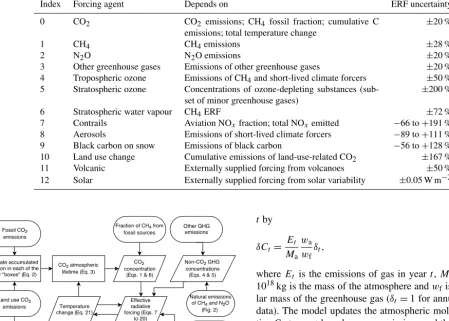
Table 3.The 13 separate forcing groups considered in FAIR v1.3 in the calculation of effective radiative forcing. The ERF uncertainty represents the 5–95 % range and is used in the generation of the large ensemble (Sect. 3). ERF uncertainties from Myhre et al. (2013b) are used except for CH4where we use the Myhre et al. (2013b) estimate inflated by the additional uncertainty in the new methane forcing relationship in Etminan et al. (2016), which also affects the uncertainty in stratospheric water vapour oxidation from methane.
Index Forcing agent Depends on ERF uncertainty
0 CO2 CO2 emissions; CH4 fossil fraction; cumulative C emissions; total temperature change
±20 %
1 CH4 CH4emissions ±28 %
2 N2O N2O emissions ±20 %
3 Other greenhouse gases Emissions of other greenhouse gases ±20 % 4 Tropospheric ozone Emissions of CH4and short-lived climate forcers ±50 % 5 Stratospheric ozone Concentrations of ozone-depleting substances
(sub-set of minor greenhouse gases)
±200 %
6 Stratospheric water vapour CH4ERF ±72 % 7 Contrails Aviation NOxfraction; total NOxemitted −66 to+191 % 8 Aerosols Emissions of short-lived climate forcers −89 to+111 % 9 Black carbon on snow Emissions of black carbon −56 to+128 % 10 Land use change Cumulative emissions of land-use-related CO2 ±167 % 11 Volcanic Externally supplied forcing from volcanoes ±50 % 12 Solar Externally supplied forcing from solar variability ±0.05 W m−2
Figure 1.Simplified overview of the FAIR v1.3 model.
we use rC=0.019 yr GtC−1 and rT=4.165 yr K−1, but in contrast to Millar et al. (2017) a pre-industrialr0=35 years is used rather than their 32.4 years. This facilitates better agreement with present-day CO2atmospheric concentrations when spun up from 1765 with historical CO2and non-CO2 emissions. This parameter combination is consistent with a present-day iIRF100 diagnosed from more complex carbon cycle models (Joos et al., 2013) with a fixed background CO2 concentration of 389 ppm.
2.1.2 Other greenhouse gases
A one-box decay model is assumed for other greenhouse gases where the sink is an exponential decay of the exist-ing gas concentration anomaly. New emissions are converted to the equivalent increase in molar mixing ratiosδCin year
tby
δCt=
Et
Ma wa wf
δt, (4)
whereEt is the emissions of gas in yeart,Ma=5.1352× 10¹⁸kg is the mass of the atmosphere andwfis the molecu-lar mass of the greenhouse gas (δt=1 for annual emissions data). The model updates the atmospheric molar mixing ra-tiosCat yeartbased on new emissions and the natural sink by
Ct=Ct−1+ 1
2(δCt−1+δCt)−Ct−1(1−exp(−1/τ )) , (5) whereτ is the atmospheric lifetime of each gas (Table 2).
ad-1800 1850 1900 1950 2000 140
150 160 170 180 190 200 210 220
(a) Methane
1800 1850 1900 1950 2000
8 9 10 11 12
(b) Nitrous oxide Prather et al. (2012) FAIR, this study
Time-varying natural emissions in FAIR
E
m
is
si
on
s,
M
t y
r
1
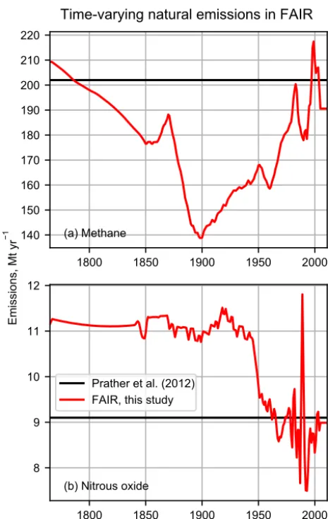
Year
Figure 2. Natural emissions of methane and nitrous oxide used in the FAIR model. Future emissions are fixed at their 2011 val-ues. Also shown are the present-day best estimates of Prather et al. (2012).
justing the atmospheric lifetime of each gas over the histor-ical period in order to match the observed concentrations at each time step.
Natural emissions of CO2are not included as the carbon cycle model is more complex than the single box used for other gases and it is assumed that natural sources and nat-ural sinks are in balance. For other greenhouse gases, natu-ral emissions are assumed to be zero except for CF4, CH3Br and CH3Cl. Pre-industrial concentrations of these three mi-nor compounds are estimated by running the 1765 emissions from Meinshausen et al. (2011b) to steady state using the lifetimes in Table 2. Unlike CH4and N2O, natural emissions of CF4, CH3Br and CH3Cl are included in the anthropogenic emissions data. In total, 31 greenhouse gas species are used (Table 2). Other than CO2, CH4 and N2O, the remaining gases can be subdivided into those covered by the Kyoto Pro-tocol (HFCs, PFCs, SF6) and the ozone-depleting substances
(ODSs) covered by the Montreal Protocol (CFCs, HCFCs, and other chlorinated and brominated compounds).
The best estimate ofτfor each gas except methane is used from AR5 (Myhre et al., 2013b, Table 8.A.1), consistent with using AR5 estimates for parameters where possible. We find that using a constant methane lifetime of 9.3 years results in reasonable levels of historical natural emissions and also agrees well with the MAGICC6-projected RCP concentra-tion scenarios in the future. The global methane lifetime of 9.3 years used is significantly lower than the perturbation lifetime of 12.4 years in AR5. This latter figure includes the feedback of methane emissions on its own lifetime due to the depletion of the OH radical, which is the main tropospheric sink for methane (a factor of 1.34; Holmes et al., 2013, also used in AR5), and is used for perturbation calculations against a constant background concentration. As emissions of OH-affecting species (NOx, non-methane volatile organic compounds (NMVOCs), CO) and temperature have varied substantially over the historical period, the background state is not constant, so the perturbation lifetime is not appropriate. 2.1.3 Methane oxidation to CO2
The oxidation of CH4produces additional CO2if it is of fos-sil origin, which is accounted for in the model. Methane is assumed to be from fossil sources if it arises from the trans-port, energy or industry sectors. A best estimate of 61 % of the methane lost through reaction with the hydroxyl radical in the troposphere (the dominant loss pathway) is converted to CO2(Boucher et al., 2009). This is treated as additional emissions of CO2:
ECH4→CO2=0.61fCH4fos CCH4−CCH4,pi
1−exp(−1/τCH4)
, (6)
wherefCH4fos is the fraction of anthropogenic methane
at-tributable to fossil sources andτCH4 is 9.3 years. Both the
fraction of methane converted (61 %) and the time series of the fraction of methane that is of fossil originfCH4fos are
user-specifiable, and RCP-derived values available from the RCP Database (2009) can be imported. The user can there-fore switch off methane oxidation by setting either of these values to zero.
Oxidation of CO and NMVOCs to CO2is not included as to not double count the carbon that is included in national CO2 emissions inventories (Daniel and Solomon, 1998; Gillenwater, 2008).
2.2 Effective radiative forcing
corre-sponds better to temperature change than “traditional” strato-spherically adjusted radiative forcing (RF) (Myhre et al., 2013b; Forster et al., 2016). Therefore, we use relationships for ERF where they exist.
2.2.1 Carbon dioxide, methane and nitrous oxide We use the updated Etminan et al. (2016) RF relationships for CO2, CH4 and N2O, which for the first time includes band overlaps between CO2and N2O. It also includes a sig-nificant upward revision of the CH4RF due to inclusion of previously neglected shortwave absorption, compared to the previous relationships of Myhre et al. (1998) used in AR5. Although Etminan et al. (2016) calculate RF, Myhre et al. (2013b) concluded that over the industrial era there was not sufficient evidence to state that ERF was significantly differ-ent from RF for these three gases, and ERF is taken to equal RF, although with a doubled uncertainty range. The Etmi-nan et al. (2016) relationships are reproduced in Eqs. (7)–(9), whereC(ppm),MandN (ppb) have been used to represent concentrations of CO2, CH4and N2O, and the subscript pi representing pre-industrial concentrations.
FCO2 = h
(−2.4×10⁻⁷)(C−Cpi)2+(7.2×10⁻⁴) |C−Cpi| −(1.05×10⁻⁴)(N+Npi)+5.36
i
×log
C
Cpi
, (7)
FN2O= h
(−4.0×10⁻⁶)(C+Cpi)+(2.1×10⁻⁶) (N+Npi)−(2.45×10⁻⁶)(M+Mpi)+0.117
i
× √
N−pNpi
, (8)
FCH4 = h
−(6.5×10⁻⁷)(M+Mpi)−(4.1×10⁻⁶) (N+Npi)+0.043×
√
M−pMpi
. (9)
Finally, a scaling to FCO2 is made to ensure that a
dou-bling of CO2 using Eq. (7) along with pre-industrial N2O concentrations equals the user-specified value ofF2×, which defaults to 3.71 W m−2.
2.2.2 Other well-mixed greenhouse gases
For all well-mixed greenhouse gases in Table 2 except CO2, CH4and N2O, the ERF is assumed to be a linear relationship of the change in gas concentrationCi since the pre-industrial era by its radiative efficiencyηi [W m−2ppb−1]:
Fi=ηi(Ci−Ci,pi);i∈ {gas indices 3,4. . .,30}, (10) where radiative efficiencies are given in Table 2,irefers to index numbers in Table 2 andCi are converted to ppb. This is an established method for small greenhouse gas forcings, also used in MAGICC.
2.2.3 Tropospheric ozone
Tropospheric ozone is formed from a complex chemical re-action chain from emissions of CH4, NOx, CO and NMVOC. Furthermore, its concentration is more variable in space and time than for the well-mixed greenhouse gases. Therefore, we do not calculate a globally averaged concentration. We use coefficients from Stevenson et al. (2013) to estimate tropospheric ozone ERF from emissions of NOx, CO and NMVOC, and concentrations of methane, assuming linear-ity between atmospheric burden and ozone forcing:
FO3tr=βCH4(CCH4−CCH4,pi)+βNOx(ENOx−ENOx,pi) +βCO(ECO−ECO,pi)+βNMVOC
(ENMVOC−ENMVOC,pi)+f (T ) (11)
and
f (T )=min{0,0.032 exp(−1.35T )−0.032}. (12) Theβ coefficients in Eq. (11) are provided in Table 4, and Eq. (12) is a small negative climate feedback, estimated using a curve fit to year 2000, 2030 and 2100 temperature changes under RCP8.5 in Stevenson et al. (2013). As Stevenson et al. (2013) used 1850 as their baseline for forcing calculations based on emissions data from Lamarque et al. (2010), in RCP scenarios adjusted coefficients can optionally be spec-ified for times prior to 1850 where “pre-industrial” anthro-pogenic emissions are taken from Skeie et al. (2011). This ensures that ERF is both equal to zero in 1765 and equal to the best estimates in Stevenson et al. (2013) for 2005. Both the differing treatment prior to 1850 and the climate feedback can optionally be switched off by the user.
2.2.4 Stratospheric ozone
The stratospheric ozone ERF is calculated using the functional relationship borrowed from Meinshausen et al. (2011a), namely
FO3st=a(b s)
c. (13)
a= −1.46×10⁻⁵,b=2.05×10⁻³andc=1.03 in Eq. (13) are fitting parameters that are found by a least-squares curve fit between Eq. (13) and the stratospheric ozone ERF time series from AR5; due to this data fitting approach, our pa-rameters differ from MAGICC.sis the equivalent effective stratospheric chlorine (EESC) from all ozone-depleting sub-stances, calculated as (Newman et al., 2007)
s=rCFC11
X
i∈ODS
nCl(i)Ci
ri
rCFC11
+45nBr(i)Ci
ri
rCFC11
. (14)
Table 4.Contribution to tropospheric ozone ERF from each precursor. Pre-industrial emissions from Skeie et al. (2011), pre-industrial CH4 from Meinshausen et al. (2011b), 1850 and 2000 emissions from Lamarque et al. (2010), and 2000 minus 1850 ERF from Stevenson et al. (2013).
Ozone forcing efficiencyβi(Eq. 11)
ERF in
Pre-2000 industrial
Species (W m−2) Pre-1850 Post-1850 value
CH4 0.178 1.73×10⁻⁴ 1.73×10⁻⁴W m−2ppb−1 722 ppb CO 0.076 4.76×10⁻⁵ 8.51×10⁻⁵W m−2(Mt yr−1)−1 170 Mt CO yr−1 NMVOC 0.044 1.88×10⁻⁴ 2.25×10⁻⁴W m−2(Mt yr−1)−1 5 Mt NMVOC yr−1 NOx 0.125 5.72×10⁻⁴ 9.08×10⁻⁴W m−2(Mt yr−1)−1 2 Mt N yr−1
Eq. (14) indicating that bromine is 45 times more effective at stratospheric ozone depletion than chlorine (Daniel et al., 1999). The concentrationsCi are expressed in ppb.
2.2.5 Stratospheric water vapour from methane oxidation
In AR5, the ERF from the stratospheric water vapour oxi-dation of methane was assumed to be 15 % of the methane ERF. This was based on the methane forcing relationship of Myhre et al. (1998), which is about 20 % lower than the Et-minan et al. (2016) methane forcing used in FAIR. As there has been no substantial revision to the stratospheric water vapour forcing, we define stratospheric water vapour ERF as 12 % of the methane ERF.
2.2.6 Contrails
Meinshausen et al. (2011b) did not include a forcing time se-ries for contrails or contrail-induced cirrus, which contribute a small positive ERF (Boucher et al., 2013). Three differ-ent methods to supply contrail ERF are available in FAIR: (1) scaling with aviation-based NOx emissions, (2) scaling with global supply of jet kerosene fuel, or (3) supplying an external forcing time series. In method 1, it is assumed that contrail ERF is proportional to the aircraft NOxemissions in a given year ENOx,avicompared to 2005 and multiplied by the 2005 ERF from Lee et al. (2009) of 0.0448 W m−2:
Fcon=
ENOx,avi ENOx,avi,2005
Fcon,2005. (15)
This gives a coefficient of Fcon,2005/ENOx,avi,2005= 0.0152 W m−2(Mt-aviNOxyr−1)−1.
Method 2 is similar, based on kerosene fuel supplied
Skerosene, as a proxy for activity data. We take a 2005 global kerosene supply of 236 Gt from International Energy Agency (2018) to anchor the forcing time series calculation:
Fcon=
Skerosene Skerosene,2005
Fcon,2005. (16)
For method 1, the past and future aviation NOxemissions from the RCP scenarios are available in FAIR. The fraction of total NOxemissions attributable to aviation is used to cal-culateENOx,aviin Eq. (15).
2.2.7 Aerosols
Aerosols have a lifetime of the order of days (Kristiansen et al., 2016), and the emissions are converted to forcing with-out an intermediate concentration step.
The aerosol ERF contains contributions from aerosol-radiation interactions (ERFari) and from aerosol–cloud inter-actions (ERFaci). ERFari includes the direct radiative effect of aerosols, in addition to rapid adjustments due to changes in the atmospheric temperature, humidity and cloud profile (formerly the semi-direct effect; Boucher et al., 2013).
We use the multi-model results from Aerocom (Myhre et al., 2013a) and assume a linear relationship between emis-sions and forcing:
Fari=γBCEBC+γOCEOC+γSOxESOx+γNOxENOx
+γNH3ENH3+γSOAENMVOC, (17)
Table 5. Contribution to ERFari from each aerosol precursor species and contribution to 2011 ERFari.
ERFari in Radiative efficiency Species 2011 (W m−2) (10−3W m−2(Mt yr−1)−1)
SOx −0.34 −6.22 (Mt S)
BC +0.13 +16.0
OC −0.05 −1.45
NH3 −0.066 −1.56 NOx −0.044 −1.17 (Mt N)
SOA −0.08 −0.38
effects). There is evidence that scattering aerosols do not ex-hibit significant semi-direct effects (Boucher et al., 2013), so the overall difference of−0.1 W m−2is assumed to be due to BC semi-direct effects. The net impact is to reduce the radiative efficiency coefficient of BC.
ERFaci describes how aerosols affect clouds in the radia-tion budget; the two main mechanisms are changes in cloud droplet size, which changes cloud albedo (Twomey, 1977) and changes in cloud lifetime and precipitation efficiency, which affects cloud fraction (Albrecht, 1989; Boucher et al., 2013). There is evidence that the ERFaci is not linear with emissions (Carslaw et al., 2013), and as such a simple linear scaling as for ERFari may not be appropriate.
In FAIR we use an emulation of the global aerosol model of Ghan et al. (2013) to estimate ERFaci from precursor emissions. The Ghan et al. (2013) method contains a series of non-linear equations that require iterative solutions and cur-rently has not been optimised for use in FAIR. We therefore emulate the ERFaci by varying the emissions of SOx and primary organic aerosol (the sum of BC and OC). Secondary organic aerosol is also an input to the model, but it is found that ERFaci is only weakly dependent on NMVOC emissions and a simple functional form could not be found and so was eliminated as a predictor.
Informed by the simple aerosol model of Stevens (2015), we use a logarithmic dependence of ERFaci on emissions that can vary both as a function of SOxand BC+OC, which represents increasing saturation of the cloud–albedo effect with increasing emissions. We find a relationship of the form
G(ESOx,EBC+OC)= −1.95 log
(1+0.0111ESOx+0.0139EBC+OC), (18)
where the coefficients in Eq. (18) are found with a least-squares optimisation routine (r2=0.938). The modelled and simulated outputs are compared in Fig. S1 in the Supplement. Equation (18) was derived from a climate model and pro-duces a present-day ERFaci that is stronger than the cen-tral estimate of−0.45 W m−2from AR5. We therefore scale Eq. (18) in order to obtain a forcing of−0.45 W m−2in 2011
under RCP4.5 emissions:
Faci= −0.45
G(E)−G(E1765) G(E2011)−G(E1765)
, (19)
whereE=(ESOx, EBC+OC) refers to emissions and a nu-merical subscript refers to a particular year. The emissions for 1750 from Skeie et al. (2011) are used for year 1765, and a linear interpolation between 1765 and 1850 is applied. 2.2.8 Black carbon on snow
The best-estimate ERF of 0.04 W m−2 in AR5 for 2011 is compared to the BC emissions in 2011 from Meinshausen et al. (2011b), with this scaling factor assumed to hold for all years. The relationship is given by
FBCsnow=0.00494EBC, (20)
whereEBCis BC emissions in Mt yr−1. 2.2.9 Land use change
Land use forcing is a result of surface albedo change (An-drews et al., 2017) and changes in evapotranspiration pat-terns (Jones et al., 2015), which is often due to deforestation for agriculture (Myhre and Myhre, 2003). Cropland has a higher albedo than the forest that it replaces, reflecting more incident solar radiation and therefore resulting in a negative ERF; additionally, deforestation in boreal regions may un-mask snow-covered ground, again increasing albedo.
Deforestation produces land-use-related CO2 emissions. The total amount of deforestation since pre-industrial times could therefore be expected to scale with cumulative land-use-related CO2emissions. This is the default approach taken in FAIR. A regression of non-fossil CO2 emissions against land use ERF in AR5 gives
Flanduse= −1.14×10⁻³
t
X
j=0
ECO2land,j, (21)
where the coefficient has units W m−2(Gt C)−1.
the forcing is a small fraction of the present-day total, and thirdly because the future trajectory of the land use forcing in the RCP datasets is very similar to that predicted by FAIR, suggesting that a dependence on cumulative land use CO2 emissions is an important component of the land use forcing in MAGICC.
Noting that this simple relationship may not be suitable in all cases, the user is free to supply their own time series of ERF from land use change. If gridded land use data are available, the transitions to and from forested land each year can be convoluted with the marginal contribution to land use forcing per square kilometre deforestation (e.g. from Jones et al., 2015).
2.2.10 Solar variability
The SOLARIS-HEPPA v3.2 solar irradiance dataset pre-pared for CMIP6 is used to generate the solar ERF, which in-cludes projections of the variation in future solar cycles from 1850 to 2300 (Matthes et al., 2017). ERF from solar forc-ing is calculated as the change in solar constant since 1850 divided by 4 (average insolation) and multiplied by 0.7 (rep-resenting planetary co-albedo). This approach is also used in Meinshausen et al. (2011b). Prior to 1850, we revert to the solar forcing from AR5.
2.2.11 Volcanic aerosol
Historical volcanic forcing is punctuated by several large eruptions that cause large but short-lived negative forcing episodes, with several smaller eruptions that cause year-to-year changes in the volcanic forcing. In order to generate a historical volcanic ERF time series, we first start with grid-ded volcanic optical depths taken from the Easy Volcanic Aerosol generator over the 1850–2014 period (Toohey et al., 2016) which will be used to drive CMIP6 models. A number of time slice experiments with various scalings of the histor-ical mean volcanic opthistor-ical depth are run in the HadGEM3-GA7.1 climate model (Walters et al., 2017), where it was found that aerosol ERF scales as−18τvol(whereτvolis glob-ally averaged volcanic aerosol optical depth at 550 nm). This scaling factor is consistent with other HadGEM models (Gre-gory et al., 2016), although weaker than the value of−26τvol adopted in AR5. The discrepancy is claimed to be due to rapid adjustments, in which case our adoption of the less neg-ative value is consistent with the ERF definition.
In the context of measuring forcing since the pre-industrial, we have to assume an “average” level of volcanic background aerosol. We therefore define the 1850–2014 pe-riod to have a mean volcanic forcing of zero. To achieve this we subtract the mean (negative) forcing from the his-torical period, resulting in a quiescent year ERF of around +0.1 W m−2. A similar approach was taken in Meinshausen et al. (2011b), with a higher quiescent year forcing of about +0.2 W m−2. Prior to 1850 we use the AR5 dataset, scaled
by 18/26 to match the differences in optical depth/forcing relationships, and from 2015 onwards volcanic forcing is de-fined to be zero. For solar and volcanic forcing, users are free to provide a custom forcing time series or to use the AR5 or RCP datasets which are both available in FAIR.
2.3 Temperature change
In simple impulse response models, forcing is related to to-tal temperature change in yeart,Tt, by a two-time constant model (Boucher and Reddy, 2008; Myhre et al., 2013b; Mil-lar et al., 2015, 2017). FAIR v1.3 takes this approach with a small modification compared to FAIR v1.0 to allow for forcing-specific efficaciesjsuch that
Tt,i=Tt−1,iexp(1/di)+
12 X
j=0
qijFj(1−exp(1/di));
i=1,2. (22)
Owing to the use of ERF rather than RF in FAIR v1.3 and its better correspondence with temperature, efficacies are as-sumed to be unity for all forcing agents except black car-bon on snow (j=9), where an efficacy of 3 is used follow-ing Bond et al. (2013). The coefficients d1 andd2 govern the slow (i=1) and fast (i=2) temperature changes from a response to forcing from the upper ocean and the deep ocean respectively (Millar et al., 2015). The total tempera-ture change in yeart is the sum of the slow and fast com-ponents, i.e.Tt=Tt,1+Tt,2.Fj represents the 13 individual forcing agents in yeart calculated in Sect. 2.2 (see also Ta-ble 3).d1 andd2default to 239 and 4.1 years which are fit to match the mean of CMIP5 models (Geoffroy et al., 2013). The coefficientsq1andq2(units K W−1m2) are determined by solving a matrix equation given transient climate response (TCR), equilibrium climate sensitivity (ECS),d1,d2and the ERF from a doubling of CO2, F2×=3.71 W m−2 (Myhre et al., 2013b):
TECS=F2×(q1+q2); (23)
TTCR=F2×
q1
1−d1
D
1−exp
−D
d1
+q2
1−d2
D
1−exp
D d2
, (24)
giving the relative contributions to the fast and slow compo-nents of the warming.D=log(2)/log(1.01)≈69.7 years is the time to a doubling of CO2with a compound 1 % per year increase in CO2concentrations.
3 Projections using a large ensemble
To test the model response to a range of forcing pathways, we perform a 100 000-member Monte Carlo simulation us-ing emissions from the RCP datasets (Meinshausen et al., 2011b). Emissions themselves are not altered from the RCP time series, but the TCR, ECS, carbon cycle response to increasing temperature (rT) and cumulative emissions (rC) along with the pre-industrial value of iIRF100 (r0), plus the ERF scale factors for each of the 13 forcing agents, are drawn from distributions. FAIR is run from 1765 (the start of the RCP emissions datasets) to 2100.
3.1 Constraint to historical temperature observations As a wide range of forcing, and thus temperature, scenar-ios can be generated, there are a proportion of ensemble members generated that fall outside the range of plausibility. We constrain the full 100 000-member ensemble (hereafter FULL) to the observed temperature change from the Cowtan and Way (2014) dataset (hereafter C&W) to assess plausibil-ity; ensemble members that satisfy the temperature constraint are designated as “not ruled out yet” (NROY) and the major-ity of the discussion of the results in Sect. 4 focuses on this dataset. We rebase all of the temperatures to the 1861–1880 mean following Richardson et al. (2016), to represent a pre-industrial state that is relatively free of volcanic eruptions but with a reasonable global coverage of temperature obser-vations. An ordinary least-squares regression of temperature change versus time from 1880 to 2016 is used to calculate the linear warming trend in each ensemble member. The regres-sion is also performed for the C&W “observational” dataset to estimate the observed warming rate. The confidence in-terval around the C&W warming rate is inflated by a factor that represents the lag-1 autocorrelation of residuals (i.e. the trend-line estimate from the regression minus the C&W “ob-servations”) which accounts for internal climate variability (Santer et al., 2008; Thompson et al., 2015) and is the same method used in AR5 to estimate linear temperature trends. The constraint is satisfied for an ensemble member if the modelled trend falls within the 5–95 % range of trend from C&W of 0.95±0.17 K.
The C&W observed warming from 1880 to 2016 is higher than the UK Met Office Hadley Centre observational dataset (HadCRUT4; Morice et al. 2012) estimate of 0.91±0.18 K for the same time frame. The infilling of grid boxes where no or limited data are available accounts for these differences, as sparse observations are typically in polar regions which warm faster than the global mean (Cowtan and Way, 2014). Under this constraint approximately 26 % of the FULL en-semble is retained in NROY.
It should be stressed that there are several issues to con-sider when attempting to derive plausible parameter sets from observational data. These include the type of observa-tional constraints to employ (Meinshausen et al., 2009), the
length of the historical record (e.g. Otto et al., 2013), the sep-aration of forced response from natural variability (Haustein et al., 2017) and assumptions surrounding prior distributions (Frame et al., 2005).
3.2 Sampling ECS and TCR
The ECS and TCR from CMIP5 models (Forster et al., 2013) are used to generate a joint log-normal distribution. Random variables are sampled using the R package MethylCapSig1 using the mean, standard deviation and correlation coeffi-cient (r=0.81) between ECS and TCR in CMIP5. A log-normal distribution is representative of distributions of ECS and TCR in the literature (Meinshausen et al., 2009; Rogelj et al., 2012; Flato et al., 2013; Millar et al., 2017). The sam-pled joint and marginal distributions are shown as black con-tours and curves in Fig. 3. We sample 100 000 ECS–TCR pairs; sampled pairs where ECS<TCR are rejected and re-drawn. A joint distribution is used because ECS and TCR are highly correlated and low values of the realised warming fraction (TCR divided by ECS) are inconsistent with mod-els and observations (Millar et al., 2015). For other sampled quantities in this section a 100 000-member ensemble is also generated.
3.3 Sampling thermal response and carbon cycle parameters
We allow F2×, the ERF due to a doubling of CO2, to as-sume a Gaussian distribution with 5–95 % confidence inter-val of 20 % around the best-estimate ERF of 3.71 W m−2 (Myhre et al., 2013b). d1 (mean 239 years, standard devi-ation 63 years) andd2 (mean 4.1 years, standard deviation 1.0 years) in Eq. (22) are also varied based on truncated Gaussian distributions (no values outside±3σ allowed, pri-marily to prevent unrealistically small or negative values of the slow responsed1). Although FAIR is able to model the re-sponse to time-varying ECS and TCR, we use time-invariant values in our ensemble.
Some uncertainty in the carbon cycle parameters is as-sumed with samples ofr0,rCandrT taken from Gaussian distributions.r0,rCandrTare given 5–95 % confidence in-tervals of 13 % of the default parameter value following Mil-lar et al. (2017).
3.4 Sampling ERF uncertainties
The uncertainty in each of the 13 forcing components is modelled following the 5–95 % confidence intervals for each forcing from AR5 (Myhre et al., 2013b, Table 8.6) in 2011 (Table 3). This is achieved by scaling the ERF values calcu-lated in Sect. 2.2; the uncertainty ranges are given in Table 3. The scaling factor is applied to the whole time series. A time-1https://cran.r-project.org/package=MethylCapSig (last access:
varying scale factor for forcing can be used, and an option is provided to exactly replicate the AR5 historical time series for each component, but we do not apply it here. Most un-certainties are assumed to be Gaussian, the exceptions being contrails and BC on snow which are log-normally distributed (with geometric standard deviations 1.92 and 1.65 respec-tively, following AR5) and aerosols which are modelled as two half-Gaussian distributions, treating values above and below the best estimate separately. These ERF uncertainties are assumed to be uncorrelated with each other.
4 Results from the NROY ensemble for the RCP scenarios
4.1 ECS and TCR
The FULL and NROY joint and marginal distributions of ECS and TCR are shown in Fig. 3.
The temperature constraint in NROY results in distribu-tions of ECS and TCR that are lower than in FULL. Some of the prior sample space in which ECS and TCR are larger than the likely AR5 ranges has been rejected in the NROY distribution. While the possibility that ECS>5 K cannot be ruled out, it appears less likely than would be inferred from CMIP5 models, although it should be stressed that time-varying feedbacks are not accounted for in this large ensem-ble, which would allow ECS to increase over time (Armour, 2017). From the marginal distributions, we estimate that ECS and TCR are 2.86 (2.01 to 4.22) K and 1.53 (1.05 to 2.41) K (median; (5–95 % range)) respectively in the NROY ensem-ble, similar to but a little more tightly constrained than the
likely AR5 (>66 % probability) ranges of 1.5 to 4.5 K and
1.0 to 2.5 K, noting that the AR5 ranges are estimated from a combination of models, observations and expert judge-ment. The ratio of TCR to ECS, the realised warming frac-tion (RWF), is approximately independent of TCR in CMIP5 models (Millar et al., 2015), and the prior distribution could alternatively be defined in terms of the TCR and RWF joint distribution, which is explored in Sect. 5. The FULL and NROY median and 5 to 95 % ranges of RWF are 0.56 (0.41 to 0.76) and 0.54 (0.40 to 0.72) respectively, which is close to the range of CMIP5 models (0.45 to 0.75, Millar et al., 2017).
4.2 Historical and future greenhouse gas concentrations
The historical (1765–2005) greenhouse gas concentrations from the RCP scenarios in Meinshausen et al. (2011b) were assimilated from observations of in situ and ice core records and represent a best estimate of the actual concentrations over this period. We therefore assume that the RCP data rep-resents the best estimate of the historical concentrations and compare our estimates from the NROY ensemble using the emissions-driven model.
The FAIR model reproduces the historical concentrations of greenhouse gases (Fig. 4). The atmospheric concentra-tions of CO2 estimated from FAIR are up to 9 ppm lower than MAGICC6 in the period 1880–1950 (Fig. 4a). A simple carbon cycle model cannot reproduce the kinks in the obser-vational CO2trend without large changes in the input emis-sions. However, between 1950 and 2005, the differences be-tween the two curves are small. The post-2005 atmospheric CO2concentrations are slightly higher than those estimated by MAGICC6 for the RCP scenarios, but the MAGICC6 con-centrations are within the uncertainty range from the NROY ensemble. FAIR projects best-estimate CO2 concentrations of 427 (413 to 443), 552 (527 to 578), 695 (661 to 731) and 979 (926 to 1040) ppm for RCP2.6, RCP4.5, RCP6 and RCP8.5 in 2100. Here, the uncertainty in CO2concentrations relates to the range of carbon cycle parameters and the tem-perature dependence on carbon uptake sampled in the large ensemble.
The historical CH4and N2O concentrations in FAIR have been tuned to agree with Meinshausen et al. (2011b) by ad-justing natural emissions as described previously (Fig. 4b, c). There are some small differences in the future CH4and N2O concentrations in the RCPs using fixed atmospheric lifetimes and constant (present-day) natural emissions.
Kyoto Protocol gases have been grouped as HFC134a-eq based on their radiative efficiency, and ODSs have been sim-ilarly grouped as CFC12-eq (Fig. 4d, e). Small differences between the models in future scenarios may be a result of the assumption of a change in the rate of the Brewer–Dobson circulation in MAGICC6 (Meinshausen et al., 2011a), which increases the efficiency of the stratospheric sink for these gases. This temperature-dependent effect is not included in FAIR. Over the historical period, the differences are a result of the natural emissions of CF4(contributing to HFC134a-eq) and CH3Br and CH3Cl (contributing to CFC12-eq) pro-viding a non-zero background state of these greenhouse gas equivalents in FAIR. In the RCP historical dataset these back-ground concentrations have not been added to the HFC134a-eq and CFC12-HFC134a-eq time series.
4.3 Historical, present and future radiative forcing
0 1 2 3 4 5 6 7 8 ECS (K)
0 1 2 3 4 5
TCR (K)
FULL joint density function
(a)
AR5 "likely" range
AR5 "likely" range
0.001
0.003
0.010
0.030
0.100
0.300 0.0
0.2 0.4 0.6
Probability density
(b) FULL distribution
NROY distribution
0.0 0.5 1.0
Probability density (c)
CMIP5 models
0.01 0.03 0.1 0.3 1.0 NROY joint density function
Figure 3. (a)Joint distributions (FULL and NROY) of ECS and TCR.(b)Marginal distributions of ECS.(c)Marginal distributions of TCR. In(a), the FULL distribution is shown with open black contours and the NROY distribution with coloured squares. Probability density is plotted on a log scale. In(b)and(c), the FULL distribution is shown as a black curve and the NROY distribution with yellow histogram bars, both plotted on a linear scale. The NROY distributions contains only those ensemble members which agree with the C&W observed historical temperatures. CMIP5 models are depicted with red circles.
a breakdown of ERF by individual gas, so the total ERF has been scaled by the ratios in the MAGICC6 time series.
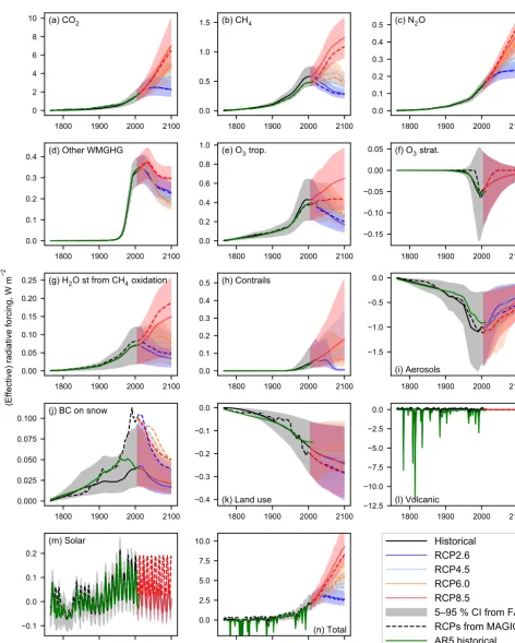
For tropospheric ozone, the Stevenson et al. (2013) rela-tionship agrees well with AR5 until around 1970, from which point it is larger than AR5. There is also a large relative dif-ference between this relationship and the MAGICC estimate in AR5 out to 2100 (Fig. 5e). The shape of the stratospheric ozone ERF curve between AR5 and MAGICC6 differs, but it can be seen that the AR5 historical ERF is well emulated as it uses the same functional relationship as AR5 (Fig. 5f). Stratospheric water vapour from methane oxidation depends on the underlying methane forcing and is similar to the AR5 time series (Fig. 5g). Contrail ERF shows a similar time evo-lution over the historical period to AR5 (Fig. 5h). Histori-cally, ERF from aviation contrails has been small but may become more substantial in the future. The median aerosol ERF in FAIR is slightly more negative than in AR5 from around 1900 to 2011 (Fig. 5i) but is less negative than the RCP projections. We reiterate here that the RCPs report RF from MAGICC rather than ERF.
1800 1900 2000 2100 400
600 800
1000 (a) CO2, ppm
1800 1900 2000 2100
1000 1500 2000 2500 3000
3500 (b) CH4, ppb
1800 1900 2000 2100
300 350 400
(c) N2O, ppb
1800 1900 2000 2100
0 250 500 750 1000
1250 (d) HFC134a-eq, ppt
1800 1900 2000 2100
0 200 400 600 800
1000 (e) CFC12-eq, ppt Historical
RCP2.6 RCP4.5 RCP6.0 RCP8.5
5–95 % CI from FAIR RCPs from MAGICC, Meinshausen et al. (2011b)
1800 1900 2000
300
350
Historical and RCP WMGHG concentrations in FAIR and MAGICC6
Concentration
Year
Figure 4.Comparison of the historical and RCP greenhouse gas concentrations in FAIR (heavy solid lines) with 5–95 % confidence intervals (shading) for CO2. Dashed lines show the concentrations from MAGICC6 (Meinshausen et al., 2011b). For CFC12-eq, the RCP4.5 and RCP6.0 lines lie underneath the RCP8.5 line.
Figure 5n shows the sum of the forcing components. The best-estimate sum of ERF follows AR5 closely over the his-torical period, which is intentional. In the RCP future sce-narios, the FAIR best estimates of ERF are higher than the corresponding RF estimates in MAGICC. This is in part due to the increased CH4, tropospheric ozone and contrail forc-ing in FAIR, and less negative total aerosol ERF. The FAIR model projects 2100 ERFs (median (5–95 % credible inter-vals)) of 2.62 (1.79 to 3.64), 4.62 (3.30 to 6.22), 5.84 (4.07 to 8.00) and 9.34 (6.84 to 12.44) W m−2for RCP2.6, RCP4.5, RCP6.0 and RCP8.5 respectively.
4.4 Relationship between forcing components, ECS and TCR
The distribution of ERF in 2017 for aerosols, greenhouse gases and the anthropogenic total in both the FULL and the NROY ensembles assuming the RCP8.5 forcing pathway is shown in Fig. 6 and Table 6. The temperature constraint in NROY permits a wider range of greenhouse gas ERF than the FULL ensemble. For aerosols, the distribution of ERF in NROY is again slightly wider than in FULL. The median es-timate of net anthropogenic ERF of 2.63 W m−2in 2017 for NROY is a little lower than the unconstrained FULL estimate of 2.73 W m−2with a wider uncertainty range.
There are negative correlations between aerosol radiative forcing and ECS/TCR (Fig. 7). A large negative aerosol forc-ing requires a high ECS to balance and recreate realistic ob-served temperatures (Forest et al., 2006). Millar et al. (2015)
highlighted the necessity of anti-correlation between TCR and aerosol forcing in observational constraints. The aerosol forcing on TCR constraint is tighter than that on ECS, ev-idenced by the narrower mass of points in the TCR plot (Fig. 7b) compared to the ECS plot (Fig. 7a). A high value for TCR (greater than 2.5 K) or ECS (greater than 5 K) is only possible with a strong negative present-day aerosol forcing (more negative than about−1.0 W m−2).
4.5 Observed and future temperature changes
1800 1900 2000 2100 0
2 4 6 8
10
(a) CO
21800 1900 2000 2100
0.0 0.5 1.0
1.5
(b) CH
41800 1900 2000 2100
0.0 0.1 0.2 0.3 0.4
0.5
(c) N
2O
1800 1900 2000 2100
0.0 0.1 0.2 0.3
0.4
(d) Other WMGHG
1800 1900 2000 2100
0.0 0.2 0.4 0.6 0.8 1.0
(e) O
3
trop.
1800 1900 2000 2100
0.15 0.10 0.05 0.00
0.05
(f) O
3strat.
1800 1900 2000 2100
0.00 0.05 0.10 0.15 0.20
0.25
(g) H
2O st from CH
4oxidation
1800 1900 2000 2100
0.0 0.1 0.2 0.3 0.4
0.5
(h) Contrails
1800 1900 2000 2100
1.5 1.0 0.5 0.0
(i) Aerosols
1800 1900 2000 2100
0.000 0.025 0.050 0.075
0.100
(j) BC on snow
1800 1900 2000 2100
0.4 0.3 0.2 0.1 0.0
(k) Land use
1800 1900 2000 2100
12.5 10.0 7.5 5.0 2.5 0.0
(l) Volcanic
1800 1900 2000 2100
0.1 0.0 0.1 0.2
(m) Solar
1800 1900 2000 2100
0.0 2.5 5.0 7.5 10.0
(n) Total
Historical
RCP2.6
RCP4.5
RCP6.0
RCP8.5
5–95 % CI from FAIR
RCPs from MAGICC
AR5 historical
(E
ffe
ct
iv
e)
ra
di
at
iv
e
fo
rc
in
g,
W
m
2
Year
Table 6.Median and 5–95 % credible intervals for effective radiative forcing from greenhouse gases, aerosols and anthropogenic total from the FULL and NROY FAIR ensembles in 2017. Anthropogenic total contains contributions from contrails, BC on snow and land use change and therefore is not equal to the sum of greenhouse gas and aerosol forcing. Compare Fig. 6.
Effective radiative forcing (W m−2)
Before temperature After temperature Forcing type constraint (FULL) constraint (NROY)
Greenhouse gases 3.69 (3.18 to 4.21) 3.68 (2.90 to 4.61) Aerosols −0.91 (−1.63 to−0.37) −0.96 (−1.65 to−0.27) Anthropogenic total 2.73 (1.85 to 3.50) 2.63 (1.74 to 3.73)
2
0
2
4
Effective radiative forcing, W m
20.0
0.2
0.4
0.6
0.8
1.0
1.2
1.4
Probability density function
Greenhouse gases
Anthropogenic
total
Aerosols
NROY ensemble
FULL ensemble
Figure 6.ERF from aerosols (blue), greenhouse gases (red) and to-tal anthropogenic (black) for present-day (2017, based on RCP8.5) runs from FAIR constrained to observed temperature change (NROY; histograms) and from prior distributions (FULL; curves); compare Myhre et al. (2013b, Fig. 8.16). Greenhouse gas forcing includes contributions from ozone and stratospheric water vapour from methane. Anthropogenic total is the sum of greenhouse gas, aerosol, contrails, BC on snow and land use change. The latter three distributions are not shown separately.
Differences between the models can arise from many sources. The results of Rogelj et al. (2012) are based on best estimates of the ECS/TCR and radiative forcing from the IPCC Fourth Assessment Report (AR4), whereas we guide FAIR using AR5 forcings. Differences between this study and Rogelj et al. (2012) could be due to differences in the his-torical radiative forcing time series. The RF over the 1861– 1880 to 2005 period, which forms the bulk of the period used to constrain the ensemble to observed temperatures, is 1.72 W m−2in Meinshausen et al. (2011b) whereas the ERF differences are 1.98 W m−2in AR5 and 1.97 W m−2in FAIR over the same period. Therefore, the same observed
tem-0
2
4
6
8
Equilibrium climate sensitivity, K
2.5
2.0
1.5
1.0
0.5
0.0
0.5
1.0
A
er
os
ol
E
R
F,
W
m
2
(a) ECS
0
1
2
3
4
5
Transient climate response, K
2.5
2.0
1.5
1.0
0.5
0.0
0.5
1.0
A
er
os
ol
E
R
F,
W
m
2
(b) TCR
10
20
30
40
50
Number of ensemble members
10
20
30
40
50
60
Number of ensemble members
Figure 7.Relationship between(a)ECS and aerosol ERF;(b)TCR and aerosol ERF for the NROY ensemble. Aerosol ERF is shown for 2017 under the RCP8.5 scenario.
1850 1900 1950 2000 2050 2100 Year
1 0 1 2 3 4 5 6 7
Temperature change relative to 1861–1880 (K)
5th percentile 16th percentile Median 84th percentile 95th percentile
(a)
Cowtan & Way reconstruction Modelled historical
RCP 2.6 RCP 4.5 RCP 6.0 RCP 8.5
RCP2.6 RCP4.5
RCP6.0 RCP8.5
FAIR, this study
Rogelj et al. (2012) 2081–2100 mean temperature change
(b)
Figure 8. (a)Historical constrained modelled temperature and future probabilistic temperature scenarios from FAIR driven by emissions and forcing from the RCPs for 1850–2100 expressed as temperature change since 1861–1880. Also shown is observed temperature from C&W.(b)Comparison of 2081–2100 mean temperature from FAIR compared to the emission-driven ensemble from MAGICC6 (Rogelj et al., 2012).
TCR priors in Meinshausen et al. (2009) and Rogelj et al. (2012) (based on AR4 but not substantially different from the CMIP5 models used in this study), a different method of constraining to observed temperatures, and different assump-tions regarding the strength of future aerosol and ozone forc-ing. The sensitivity to some of these assumptions is tested in Sect. 5.
4.6 Transient climate response to emissions
There is an approximately linear relationship between cumu-lative CO2emissions and temperature, independent of the ac-tual emissions pathway taken, provided temperature is still increasing (Allen et al., 2009; Collins et al., 2013). Using this linearity we can diagnose the transient climate response to emissions (TCRE), defined as the change in temperature for a 1000 Gt cumulative emission of carbon.
We show both the TCRE assuming CO2forcing alone and the temperature change due to all forcing agents but
mea-sured against cumulative carbon emissions (Fig. 9). When including the effect of non-CO2forcing on the total temper-ature change, the tempertemper-ature response is substantially larger than for CO2forcing alone. This indicates that a smaller cu-mulative CO2 emission is required to reach the same tem-perature change and is a result of the total non-CO2forcing being positive. This same conclusion was reached in Collins et al. (2013) when assessing a suite of earth system models.
To determine the TCRE we run FAIR in CO2-only mode. We measure cumulative CO2 emissions and temperature change since 1870, as this is the date from which reliable es-timates of carbon emissions start (Le Quéré et al., 2016) and is also at the centre of the 1861–1880 period used to evaluate temperature changes.
0 250 500 750 1000 1250 1500 1750 2000 Cumulative carbon emissions since 1870, Gt C
1 0 1 2 3 4 5 6
Temperature change since 1870, K
Historical RCP 8.5, all forcing
RCP 8.5, CO2 forcing
5–95 % CI from all forcing 5–95 % CI from CO forcing2
Figure 9.Transient climate response to CO2emissions (TCRE) for FAIR based on RCP8.5 for all forcing (red) and for CO2-only forc-ing (black).
2013). Towards higher cumulative CO2emissions in RCP8.5 the temperature response has a slightly concave shape. The slight (rather than moderate) downward curvature is also present in CMIP5 earth system models, as the increase in airborne fraction of CO2with emissions almost cancels out the logarithmic relationship between CO2concentration and temperature (Millar et al., 2016).
4.7 Top of atmosphere energy imbalance
The top of atmosphere energy imbalanceNcan be diagnosed from (Forster et al., 2013)
N =F−λT , (25)
where λ is the climate feedback parameter and λ=
F2×/ECS. In Fig. 10 we compare FAIR model outputs from the NROY ensemble under RCP4.5 to observations of the earth’s energy imbalance from satellites (Clouds and the Earth’s Radiant Energy System; CERES) and from the array of Argo floats (Argo, 2000), which measure ocean tempera-ture which is the largest component of the change in earth’s energy budget. Both datasets are taken from Johnson et al. (2016).
For most years from 2001 to 2015, the net energy bal-ance from CERES is within the uncertainty range estimated from the FAIR NROY ensemble. The Argo estimate of N
is more variable prior to 2005, after which coverage of the Argo floats saw a large increase (Johnson et al., 2016). From 2005 onwards, all Argo estimates but one fall inside the cred-ible range of FAIR estimates. Both CERES and Argo obser-vations from 2005 onwards are clustered towards the lower half of the credible range from FAIR, which may indicate that ECS over the 2005–2015 period could be towards the lower end of the credible range estimated from the NROY ensemble.
2002 2004 2006 2008 2010 2012 2014
Year 1.0
0.5 0.0 0.5 1.0 1.5 2.0 2.5
To
p
of
a
tm
os
ph
er
e
en
er
gy
im
ba
la
nc
e,
W
m
2
FAIR CERES ARGO
Figure 10.Comparison of earth’s energy imbalanceNto observa-tions from Argo and CERES, from Johnson et al. (2016).
5 Sensitivity to prior distributions and constraints To determine the robustness of the results of the NROY en-semble, the input assumptions were varied or the ensemble members subjected to a different constraint as described in this section. The results are summarised in Tables 7, 8 and 9. 5.1 Prior distributions of ECS and TCR
The prior distributions of ECS and TCR have a large influ-ence on the posterior distributions attained (Pueyo, 2012). Here we test the dependence of the shape of the posterior distributions of ECS and TCR in the constrained samples on the choice of prior distributions.
As the RWF is approximately independent of TCR we use an alternative prior starting with the distributions of TCR and RWF. Noting the analysis of Collins et al. (2013), the likely AR5 range of TCR of 1.0 to 2.5 K is taken to be most probable, with values between 0.5–1.0 K and 2.5–3.5 K pos-sible but unlikely. A trapezoidal distribution in TCR with these limits is constructed, therefore not expressing any prior judgement about the most likely value of TCR within the likely AR5 range. The RWF is sampled from a Gaussian distribution with mean 0.6 and 5–95 % range of 0.45–0.75 following Millar et al. (2017), truncated to fall within the 0.2–1.0 range. These ranges are subjective choices based on evidence from CMIP5 models. The posterior distribution of ECS in particular can be sensitive to the choice of prior dis-tribution (Frame et al., 2005; Pueyo, 2012). Figure S2 shows the alternative prior distributions and the posteriors obtained as a result of constraining to the C&W observed tempera-tures.
Table 7.Sensitivity in the ECS, TCR and TCRE to variations in the underlying assumptions in the FAIR large ensemble. For the sensitivity experiments the section number in the paper describing the change is given. The “accepted” column details the proportion of the 100 000-member FULL ensemble that satisfied the specified temperature constraint.
Variation (section) Accepted ECS (K) TCR (K) TCRE (K (Eg C)−1)
5 % 50 % 95 % 5 % 50 % 95 % 5 % 50 % 95 %
C&W temperature constraint (NROY) 26.1 % 2.01 2.86 4.22 1.05 1.53 2.41 0.96 1.40 2.23 C&W with alternative ECS/TCR prior (5.1) 21.6 % 1.57 2.62 4.76 0.99 1.55 2.68 0.89 1.35 2.55 C&W withF2×=3.44 W m−2(5.2) 24.9 % 1.99 2.84 4.22 1.03 1.52 2.41 0.93 1.36 2.15 HadCRUT4 temperature constraint (5.3) 26.4 % 1.97 2.82 4.19 1.02 1.51 2.38 0.93 1.37 2.21 GISTEMP temperature constraint (5.3) 33.2 % 2.03 2.89 4.26 1.06 1.56 2.44 0.97 1.42 2.27 Berkeley Earth temperature constraint (5.3) 23.4 % 2.11 2.97 4.32 1.13 1.61 2.48 1.02 1.47 2.30 NOAA temperature constraint (5.3) 35.2 % 1.98 2.85 4.22 1.03 1.52 2.41 0.93 1.39 2.23 No temperature constraint (FULL) 100 % 2.00 3.11 4.86 1.01 1.73 2.96 0.91 1.58 2.78
Table 8.Sensitivity in the effective radiative forcing to variations in the underlying assumptions in the FAIR large ensemble.
Variation Effective radiative forcing in 2100, W m−2
RCP 2.6 RCP 4.5 RCP 6.0 RCP 8.5
5 % 50 % 95 % 5 % 50 % 95 % 5 % 50 % 95 % 5 % 50 % 95 %
C&W temperature constraint (NROY) 1.79 2.62 3.64 3.30 4.62 6.22 4.07 5.84 8.00 6.84 9.34 12.40 C&W with alternative ECS/TCR prior 1.76 2.61 3.68 3.27 4.61 6.25 4.04 5.84 8.04 6.81 9.34 12.42 C&W withF2×=3.44 W m−2 1.67 2.45 3.40 3.12 4.34 5.85 3.83 5.47 7.48 6.51 8.83 11.69 HadCRUT4 temperature constraint 1.76 2.59 3.59 3.27 4.57 6.17 4.03 5.78 7.93 6.78 9.26 12.28 GISTEMP temperature constraint 1.80 2.64 3.67 3.31 4.63 6.27 4.09 5.87 8.05 6.86 9.37 12.45 Berkeley Earth temperature constraint 1.85 2.70 3.73 3.36 4.71 6.36 4.16 5.97 8.17 6.94 9.50 12.58 NOAA temperature constraint 1.77 2.60 3.62 3.27 4.59 6.21 4.04 5.80 7.98 6.79 9.29 12.36 No temperature constraint (FULL) 1.65 2.67 3.90 3.17 4.67 6.55 3.91 5.91 8.40 6.66 9.42 12.85
the wider range of ECS and TCR admitted in the posterior distributions (Table 7) using this alternative prior.
5.2 ERF from a doubling of CO2
The canonical RF value of F2×=3.71 W m−2 may not be applicable when considering all land surface and tropo-spheric rapid adjustments in the definition of ERF. For CO2 forcing, rapid adjustments include cloud changes that are not driven by temperature change (Gregory and Webb, 2008) and land surface adjustments consequential to plant stomatal con-ductance (Doutriaux-Boucher et al., 2009). The mean ERF for a doubling of CO2 in CMIP5 models was found to be 3.44 W m−2(Forster et al., 2013). The simulation is repeated with this new lower ERF value for a doubling of CO2, with the same uncertainty of 20 %.
It is found that this lower value ofF2×slightly lowers the best estimate and credible range of ECS, TCR and ERF, but the temperature change under the RCP scenarios is higher than in NROY due to non-CO2forcings. This behaviour can be analysed with the help of Eq. (25). In equilibrium states, the top of atmosphere (TOA) energy imbalance N=0 and Eq. (25) is rearranged to yieldT =F2×/λ. IfF2×is found
to take a lower value and ensemble members are constrained to the same observed temperature, then the climate sensitiv-ity 1/λmust be higher to compensate for this. Therefore, the same positive future non-CO2forcing time series will pro-duce higher temperatures in the future.
5.3 Historical temperature constraint
Historical temperatures were also constrained using the Had-CRUT4 dataset without infilling (Morice et al., 2012), along with the GISTEMP (Hansen et al., 2010), Berkeley Earth (Berkeley Earth, 2017) and NOAA (Zhang et al., 2017) ob-servational datasets. The linear 1880–2016 trends are 0.91± 0.18 K, 0.99±0.22 K, 1.07±0.16 K and 0.93±0.24 K respec-tively. All datasets, including C&W (0.95±0.17 K), were ac-cessed on 17 October 2017.
tem-Table 9.Sensitivity in the 2100 temperature change in RCP scenarios to variations in the underlying assumptions in the FAIR large ensemble.
Variation Temperature change in 2100 from 1861 to 1880 mean, K
RCP 2.6 RCP 4.5 RCP 6.0 RCP 8.5
5 % 50 % 95 % 5 % 50 % 95 % 5 % 50 % 95 % 5 % 50 % 95 %
C&W temperature constraint (NROY) 1.10 1.48 2.09 1.73 2.37 3.45 2.08 2.84 4.14 3.11 4.33 6.50 C&W with alternative ECS/TCR prior 0.95 1.42 2.26 1.52 2.31 3.83 1.86 2.80 4.59 2.82 4.29 7.24 C&W withF2×=3.44 W m−2 1.10 1.49 2.11 1.73 2.39 3.51 2.07 2.85 4.19 3.13 4.38 6.63 HadCRUT4 temperature constraint 1.06 1.44 2.05 1.67 2.31 3.39 2.00 2.77 4.07 3.01 4.22 6.40 GISTEMP temperature constraint 1.11 1.51 2.14 1.74 2.42 3.53 2.09 2.90 4.25 3.14 4.42 6.62 Berkeley Earth temperature constraint 1.19 1.59 2.20 1.88 2.52 3.62 2.27 3.03 4.36 3.39 4.60 6.79 NOAA temperature constraint 1.06 1.47 2.09 1.67 2.35 3.46 2.00 2.81 4.15 3.01 4.29 6.51 No temperature constraint (FULL) 0.92 1.66 2.97 1.52 2.66 4.73 1.81 3.20 5.75 2.80 4.90 8.72
peratures under the RCP scenarios. Using the FULL ensem-ble, however, leads to wide uncertainty bounds and higher median estimates of these diagnosed parameters than using any of the constrained ensembles. Therefore, using a histor-ical temperature constraint rejects parameter combinations that produce larger future temperature changes.
6 Conclusions
We present a simple model, FAIR v1.3, that calculates global temperature change, effective radiative forcing from a vari-ety of drivers and concentrations of greenhouse gases. The emissions-based model is based on the FAIR v1.0 carbon-cycle–climate model with an extension for emissions of non-CO2greenhouse gases, ozone precursors and aerosols. This version of FAIR, which is tuned to the effective radiative forcing time series in AR5 over the historical period, pro-vides ERFs that are close to the target radiative forcings from the RCP scenarios in 2100. FAIR was not tuned to emulate the radiative forcing in the MAGICC6 model; however, it closely matches the concentrations of greenhouse gases pro-jected in that model.
Within FAIR, the response of the carbon cycle model can be adjusted via the rate of uptake of carbon by land and ocean processes parameterised as a function of total temperature change and cumulative carbon emissions (iIRF100). Emis-sions and concentrations are converted to effective radiative forcing and the relationship of ERF to temperature change is governed by the TCR, ECS and the efficacy of each of the 13 separate forcing categories considered in the model. The em-ulation of specific earth system models is therefore possible as discussed by Millar et al. (2017).
Using a correlated joint log-normal prior distribution of ECS and TCR based on CMIP5 models, running a 100 000-member ensemble in FAIR, and keeping only those ensem-ble members that match the rate of temperature change from 1880–2016 in C&W (the “not ruled out yet” or NROY en-semble), we find the median and 5–95 % credible ranges of
ECS and TCR to be 2.86 (2.01 to 4.22) K and 1.53 (1.05 to 2.41) K respectively. The transient climate response to CO2 emissions (TCRE) is diagnosed from a CO2-only ensemble and found to be 1.40 (0.96 to 2.23) K (1000 GtC)−1. These ranges are similar to the IPCC likely AR5 ranges for ECS, TCR and TCRE, albeit with tighter credible bounds. The NROY best estimates and ranges are not very sensitive to a lower estimate of the ERF from a doubling of CO2or a dif-ferent observational temperature dataset to constrain the his-torical temperature change rather than the Cowtan and Way (2014) dataset. They are more sensitive to the prior distribu-tion of ECS and TCR, particularly for the constraint on ECS. All methods of constraint lead to lower median and credible range estimates of ECS, TCR and TCRE than not constrain-ing to temperature at all (the FULL ensemble, with input pa-rameters estimated from the distribution of CMIP5 models and ERF uncertainties based on AR5 estimates).
Our estimate of TCR is not as low as the range derived by Otto et al. (2013) from observational constraints (0.9 to 2.0 K). Similarly our best estimate of ECS is higher than the estimate provided by Gregory and Andrews (2016) of around 2 K using observed sea-surface temperatures and sea ice in two atmosphere-only general circulation models (GCMs). While we cannot absolutely rule out values of ECS greater than 5 K or TCR greater than 2.5 K, this would require a strong present-day aerosol forcing (at least as negative as −1.0 W m−2) to balance. Progress towards tightening these upper bounds could therefore be achieved with a better un-derstanding of the present-day aerosol forcing (Stevens et al., 2016).