Iterative Bayesian denoising based on variance stabilization using Contourlet Transform with Sharp Frequency Localization: application to EFTEM images

R E S E A R C H A R T I C L E

Open Access

Iterative Bayesian denoising based on

variance stabilization using Contourlet

Transform with Sharp Frequency

Localization: application to EFTEM images

Soumia Sid Ahmed

, Zoubeida Messali

, Larbi Boubchir

, Ahmed Bouridane

, Sergio Marco

and Cédric Messaoudi

Abstract

Background: Due to the presence of high noise level in tomographic series of energy filtered transmission electron

microscopy (EFTEM) images, alignment and 3D reconstruction steps become so difficult. To improve the alignment process which will in turn allow a more accurate and better three dimensional tomography reconstructions, a preprocessing step should be applied to the EFTEM data series.

Results: Experiments with real EFTEM data series at low SNR, show the feasibility and the accuracy of the proposed

denoising approach being competitive with the best existing methods for Poisson image denoising. The effectiveness of the proposed denoising approach is thanks to the use of a nonparametric Bayesian estimation in the Contourlet Transform with Sharp Frequency Localization Domain (CTSD) and variance stabilizing transformation (VST). Furthermore, the optimal inverse Anscome transformation to obtain the final estimate of the denoised images, has allowed an accurate tomography reconstruction.

Conclusion: The proposed approach provides qualitative information on the 3D distribution of individual chemical

elements on the considered sample.

Keywords: Image denoising, Variance stabilizing transformation, Bayesian estimation, Contourlet transform, EFTEM

Backround

Transmission Electron Tomography (TET) is one of the most widely used methods for structural analysis in biol-ogy and is capable to reveal subcellular structures at the nanometric scale. The combination of TET with chem-ical mapping (such energy filter transmission electron microscopy: EFTEM) gives qualitative information on the distribution of the chemical elements by the generation of 3D chemical maps in the analyzed samples [1] thus over-coming the limitation of 2D maps. In an EFTEM mode, the transmitted electrons lose different energies according

*Correspondence:[email protected]

†_{Soumia Sid Ahmed, Zoubeida Messali and Larbi Boubchir contributed}

equally to this work.

2_{LIASD research Lab., Department of Computer Science, University of Paris 8,}

Saint-Denis, France

Full list of author information is available at the end of the article

to their interaction with the atoms present in the sample. These energies are characteristic of each type of inter-action where electron magnetic fields can be used to separate these electrons. Thus, it is possible to construct a filtered image using only those electrons having lost a precise energy. This approach allows for the computation of elemental maps as images calculated after removing the unspecific signals. The inherent presence of low signal-to-noise ratio (SNR) in biological specimens when an EFTEM is performed, remains a major issue to generate high resolution and good quality EFTEM-3D maps. thus limiting the use of 3D chemical mapping in biology. This paper aims to improve the quality of the acquired images by applying denoising approaches respecting the physical significance of the pixel values of EFTEM maps (which represent the number of electrons having lost a character-istic energy) to produce 3D chemical maps of very high

first one comes from the sensor such as the CCD cam-era, while the second comes from the inelastic interactions of the electrons beam with the specimen. The noise from the camera is dominant and is modeled as a Poisson process. Therefore, we have assumed that the EFTEM images are corrupted by additive Poisson noise. Therefore, EFTEM images are denoised using a Bayesian denoiser in the Contourlet Transform with Sharp Frequency Local-ization (CTSD) [6] domain iteratively in order to improve progressively the effectiveness of the Anscombe trans-formation (i.e. variance stabilizing transtrans-formation VST) [7, 8]. Furthermore, we demonstrate that the assump-tion of a Poisson noise with a combinaassump-tion of a Bayesian denoiser in CTSD domain and the Anscombe transformation allow for a significant enhancement of the chemical map computation which in turn will enhance the 3D reconstructed volume of EFTEM images with a computational cost at worst twice that of our previous non-iterative Bayesian denoiser [9]. We demonstrate through experiments with real EFTEM images contaminated by additive Poisson noise that the performance of the proposed method substan-tially surpasses that of previously published meth-ods. The proposed method is qualitatively evaluated in an observer study to assess the improvement of 3-D visualizations of EFTEM series and quantitatively in terms of SNR.

This paper is organized as follows: “Results” section defines the evaluation criteria considered and the com-puted maps including a comparative analysis of the performance of the proposed denoising method in this study with previously published denoising methods [3,9–12] on different real data sets. Furthermore, numer-ical experiments in this section are presented to demon-strate the effectiveness of the proposed method over recent denoising approaches. “Discussion” section dis-cusses the performance and effectiveness of the proposed method. Concluding remarks are given in “Conclusion” section. Finally, “Methods” section describes first the EFTEM images used in this work and which are a specific data collected at different energies 650, 680 and 710 eV from a biological sample, namely Fonse-caea pedrosoi. It also describes the propose iterative

only chosen denoising methods using the same Bayesian denoiser with the scale-mixture approximation to the alpha-stable prior, called "α-stable mixture" in different domains. The three domains that we have considered are the Wavelet transform [13], the Contourlet transform [14] and the CTSD domains, respectively, as shown in the workflow at the end of this paper (Fig. 5). Knowing that the bloc of Hot spot in the workflow represents a pre-processing of removing the aberrant pixels from the EFTEM images using the ImageJ plugin EFTEM-TomoJ [1,15]. The EFTEM-TomoJ and TomoJ blocs are the plu-gins under ImageJ used to compute the elemental map and the 3D tomography reconstruction of our tilt series respectively.

Since the aim of this study is to enhance the qual-ity of the reconstructed volume of the sample, we have not assessed our proposed method on the 3D volumes for evaluating its effectiveness before and after doing the reconstruction. In addition to the visual quality of the 3D volumes, we have used two evaluations criteria: the SNR and the weber contrast (CW) [16] of the iron

aggre-gates present at the cell wall (signal) in the 3D volume using the resin area as the background. Both the SNR and

CW are calculated using the projections from the

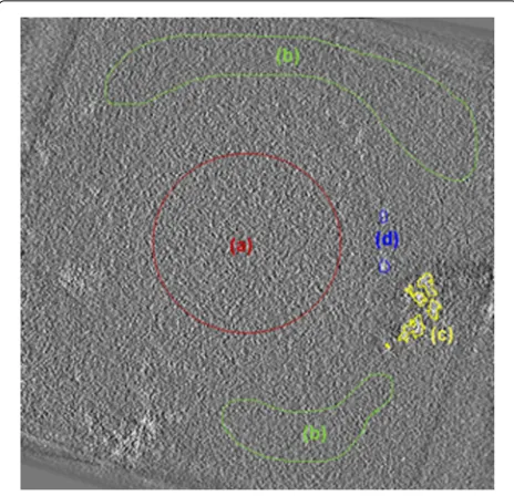
cen-tral plans (20 to 38) which contains the aggregates in the reconstructed volume. Figure1shows the central plan of the reconstructed volume and the different areas before denoising.

The SNR was calculated in decibels using the following equation:

SNR_wall=10 log₁₀

W−R

σresin

2

(1)

whereWandRare the average values of the amplitude of the net wall signal and the resin, respectively,αresinis the

standard deviation of the resin.

In order to calculate the weber contrast in the wall area, we used the following formula:

CW =

W−R R

Fig. 1Central plane (number 31 of sections 0 to 63) of the reconstructed volume before denoising. The gray levels are voxels proportional directly to the quantity of the present iron.acytoplasm,

bresin,ciron aggregate areadiron aggregates on the cell wall which are considered as the useful signal and is used to evaluate the different algorithms

where CW is the contrast in the wall area, W and R

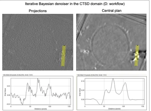
are the mean values of the pixels in the wall and resin zones, respectively. The detection of the iron aggregate is an important task for further following biologic process. The texture of the different regions in the EFTEM image isn’t considered in this work. Figure 2 shows the visual results of the central plan and the eighteen projections of the reconstructed volume using the estimated images for each denoising method. One can clearly see that the visual quality of the proposed iterative Bayesian denoiser in the CTSD domain with the VST for the Poisson noise outperforms the considered denoising methods. By com-bining the noisy observation with a previously obtained estimate of the noise free data, our denoiser overcomes the limitations of our original Bayesian denoiser in [9]. The zooming on a textured area of the sample proves not only that our denoiser ensures a good compromise between the noise rejection and the conservation of the finer details in the image, but also there are some details that were hidden due to the noise but after the denoising they became visually clear as shown in Fig.3.

To demonstrate that the proposed denoising process maintain the contents of the original images, we plot the profile of the images before and after the proposed denois-ing process, as we did in our previous work [17], usdenois-ing ImageJ 1.48v. In Fig.4, we plot a 26-pixel integrated inten-sity profile along the region of interest ROI ’iron aggregate

area’ on both original noisy images and denoised images. We clearly observe that the contents of the denoised images are not affected.

Figure5summarizes all the methods that we have used in this study where (A) is the reference. We reconstructed the 3D volume of the original images (i.e. without denois-ing) to compare its quality with the quality of those with denoising. The outputs of (B), (C), (D) and (E) are the tilt series denoised using the Bayesian denoiser in the wavelet, the contourlet SD, the contourlet SD in iterative way and in the contourlet domains, respectively. The bloc of Hot spot in the workflow represents a pre-processing of removing the aberrant pixels from the EFTEM images using the ImageJ plugin EFTEMTomoJ [1,14]. This step is applied before and after the denoising step to make the alignement process during the reconstruction easier. The EFTEM-TomoJ and TomoJ blocs are the plugins under ImageJ used to compute the elemental map using the 3-window technique which requires three energy-filtered images and the 3D tomography reconstruction of our tilt series, respectively.

To measure performance improvement, we have cal-culated the SNR (Table 1) and the weber contrast CW

using the reconstructed volumes before and after denois-ing of the whole database (228 images) for each denoisdenois-ing method, which means 912 images total. After analysing the results, one can see that the SNR and the CW are

enhanced in all the applied methods and the Bayesian estimator in the wavelet and the contourlet transform domains is comparable to the Bayesian estimator in the CTSD domain. One can also notice that the proposed iter-ative denoiser outperforms the previous methods, espe-cially our previous work [9] and gives much better results in terms of both SNR andCW, where the SNR is enhanced

by about 11 dB compared to the Bayesian estimator in the CTSD domain [9]. The main reason is that the iter-ative combination with a previous estimate refines the stabilization and helps to tackle the problem of the low SNR for this type of images. These findings suggest that

Table 1SNR and contrastCWof the wall area

Projections SNRwall CW W R resinstd

Original 2.66 0.06 21.30 20.00 0.96

Baysian denoiser in WT domain

9.99 0.10 22.01 19.95 0.65

Baysian denoiser in CTSD domain

8.05 0.07 21.33 19.91 0.56

Baysian denoiser in CT domain

9.01 0.08 21.63 19.91 0.61

Proposed iterative Bayesian denoiser with VST in CTSD domain

19.21 0.10 22.08 19.95 0.23

Fig. 2Results of the iterative denoising process on images. The charts correspond to profiles obtained from the lines drawn in each image

the proposed iterative Bayesian denoising in the CTSD domain with VST is an accurate method adapted to cap-ture the fine details that are hidden because of the Poisson noise.

We should note, that the accurate and judicious assump-tion of the Poisson distribuassump-tion instead of the Gaussian one to model the additive noise in the observation data EFTEM, helped to improve the considered Bayesian esti-mators.

Discussion

After analysing the results, one can see that the SNR and the CW are enhanced in all the applied methods and the Bayesian estimator in the wavelet and the contourlet transform domains is comparable to the Bayesian esti-mator in the CTSD domain. One can also notice that the proposed iterative denoiser outperforms the previous methods, especially our previous work [9] and gives much better results in terms of both SNR and CW, where the

SNR is enhanced by about 11 dB compared to the Bayesian estimator in the CTSD domain [9]. The main reason is that the iterative combination with a previous estimate refines the stabilization and helps to tackle the problem of the low SNR for this type of images. These findings sug-gest that the proposed iterative Bayesian denoising in the CTSD domain with VST is an accurate method adapted to capture the fine details that are hidden because of the Poisson noise. We should note, that the accurate and judi-cious assumption of the Poisson distribution instead of the Gaussian one to model the additive noise in the obser-vation data EFTEM, helped to improve the considered Bayesian estimators.

Conclusion

Fig. 4Visual comparison of the projections of the EFTEM images using the iterative Bayesian denoising in the CTSD domain with VST for the Poisson noise and the Bayesian estimator in the CTSD domain [9]. The image was zoomed on a textured area of theFonsecaea pedrosoi, where the yellow arrows indicate the iron aggregates on the cell wall

image) refines the stabilization which leads to a bet-ter quality of the images in bet-terms of a higher SNR and contrast which in turn enhances the 3D tomographic reconstruction. In order to illustrate the potential of the proposed denoising method and analyze the importance of embedding the VST framework within the iterations, we have compared our results using simplified version of the developed algorithm (without iteration and without VST) in different domains with the proposed denois-ing algorithm. After applydenois-ing the non iterative Bayesian estimator in the different domains, we have obtained

good results where the SNR is considerably enhanced. To further address the problems associated with miss-ing details in the denoised images, we have refined our previous method by taking into account the geometri-cal information of the images (i.e. contours). Therefore, we have applied iteratively the Bayesian denoiser in the CTSD domain where we have used the Anscombe trans-form to normalize the image noise. Then denoising the EFTEM images with a nonlinear nonparametric Bayesian estimator is performed to reconstruct the images to their original range via an optimal inverse transformation. This

algorithm gave us better results as shown in Fig.2, where details hidden after previous denoising approach, are now preserved, as shown in Fig. 3. Our future will focus on studying other nonparametric Bayesian estimators, in particular, the estimator based on Bessel-K-form (BKF) density [18–20].

Methods Nature of data

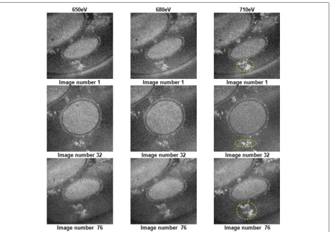
The denoising methods were applied on experimen-tal data collected from a biological sample (Fonsecaea pedrosoi). These experimental data consist of EFTEM tomographic tilt series acquired using a Saxton scheme from -60° to 60° with TEMography Software from JEOL Ltd (interested readers are referred to [1]. In our case, we have used three series of different energies 650, 680 (cor-responding to pre-edges representing the background of the chemical element Fe) and 710 eV (corresponding to the Fe L2 peak representing the characteristic iron signal) with an energy window of 20 eV; each one containing 76 gray-scale images of size 512×512 pixels each. Figure6 shows three examples of images number 1, 32 and 76 from

each series at different energies (650, 680 and 710 eV) and three angles (-60°, 0° and 60°). Three principal image areas are considered in quantitative assessments, namely: (a) cytoplasm, (b) resin, (c) iron aggregate area and iron aggregates on the cell wall. The yellow circles in the 710 eV images corresponds to iron aggregates, which are con-sidered as the useful signal and are used to evaluate the different algorithms.

Proposed denoiser

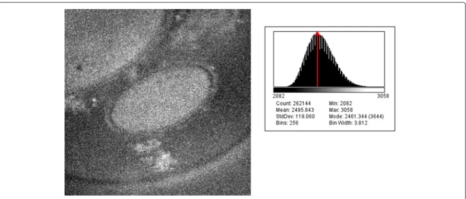
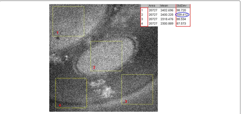
This paper proposes to denoise the EFTEM images using an iterative way. Our inputs are EFTEM images affected by an additive Poisson noise imaged at different energies. The histogram of the noisy images is positively skewed as shown in Fig. 7. To denoise them, we apply a VST approach to standardize the image noise as the first step. Then, we calculate the standard deviation (STD) of differ-ent regions in the same image as shown in Fig.8, in order to confirm that it is not stable as it should be in the case of a Poisson noise. This explains why we need firstly to apply the VST to standardize the image noise. Then, we denoise the images by considering them like they areas

Fig. 7Histogram of EFTEM image(The EFTEM image number 06 of the 650eV tilt series with its corresponding histogram)

being contaminated with an additive white Gaussian noise (AWGN). The iterative proposed algorithm is based on a nonparametric denoising method in the CTSD domain. Once obtaining After getting the denoised images, we apply the optimal inverse of the VST using ; in our case we used the most common one for this purpose which is the Anscombe transformation (AT) [7].

The Anscombe transform converts a Poisson noise to Gaussian noise with variance 1 [7] so, from a mathemati-cal viewpoint, our model is

y=x+ε (3)

where yandx are respectively the noisy EFTEM image and the original clean image to recover,εis an additive Gaussian noise.

Basic assumption

Our input is a noisy EFTEM imageycomposed of pix-els y(m,n), modeled as an independent realization of a Poisson process with parameterx(m,n)≥0:

y(m,n)∼P(y(m,n)|x(m,n))

=

x(m,n)y(m,n)_e−x(m,n)

y(m,n)! y∈N∪ {0}

0 elsewhere

(4)

knowing that the mean and variance ofycoincide and are equal tox:

E y|x=var y|x=x (5)

Proposed iterative algorithm

Our goal is to homogenize the noise variance in all image regions. Therefore, we first apply the Anscombe for-ward transformation to each image. This transformation step normalizes the image noise [21, 22] and yields an imagea(y):

a(y)=yAT =2

y+3/8 (6)

The observations a(y) can be treated as corrupted by AWGN with homogeneous variance. After apply-ing AT, we apply a Bayesian denoiser in the CTSD domain(BDCTSD), proposed in our previous work [9] to

enhance the observed images in terms of visual qual-ity, contrast and SNR. For the sake of clarqual-ity, we first describe the Bayesian denoiser in this section. The trans-formed observed image is represented in the contourlet-SD domain by:

CTSDk(a)=sk+k (7)

whereCTSDk(a),skandkare the contourlet coefficients

in thekthdirectional subband of the observed noisy image, noise-free image and noise respectively.

Because the contourlet has the similar characteristics as the wavelet, so we can straightforwardly extended the Bayesian denoiser proposed in the wavelet domain [11,12], into the contourlet domain.

In our study, similarly to the wavelet domain, the applied Bayesian denoiser in the contourlet domain is based on adapting a prior statistical model for sk and then

imposes it on the contourlet coefficients to describe their distribution.

Fig. 8Standard deviation values (STD) in different regions of an EFTEM image

theα-stable prior with the scale mixture approximation, called "α-stable mixture" to model the contourlet subband coefficients [9].

The denoised contourlet coefficients of the image are then estimated by theL2-based Bayes rules, which corre-spond to posterior conditional mean (PCM) estimate as shown in our previous work [9]. The inverse contourlet transform is computed through the processed contourlet coefficients to get the denoised image).

The Bayesian denoiserBDCTSD, is viewed as an efficient

filter for AWGN. If denoising is ideal, we have:

BDCTSD(yAT)=BDCTSD(a(y))=E[yAT|y] (8)

The so-called exact unbiased inverse of a [7]

Iap:E

a(y)|x→Ey|x=x (9)

is used to generate the denoised image to the original range ofy, thus yielding an estimate ofx:

x=Iap(BDCTSD(yAT)) (10)

whereBDCTSDdenotes the Bayesian denoiser in the CTSD

proposed in [9].

The main steps of the proposed denoising algorithm are as follows:

• Step 1:Normalize the variance noise of the observed EFTEM data by applying the VST to each image of the three tilt series. This step produces an EFTEM data set such that each imageyATlike it is contaminated with AWGN.

• Step 2:Apply the Bayesian denoiser in the CTSD domain(BDCTSD)[9] to the transformed noisy data. The(BDCTSD)consists on: (a) calculate the CTSD coefficients of theyAT, (b) denoise the detail coefficients of the CTSD at each scale and each orientation, (c) reconstruct the denoised image by applying the inverse CTSD to the estimated coefficients. This is done for each image separately. We should recall that for the Bayesian denoiser in the contourlet transform and the contourlet-SD, we selected the number of levels for the Directional Filter Bank (DFB) at each pyramidal level equal to (2, 3, 4, 5) pkva filters and we did not downsample the low-pass subband at the first level of decomposition, based on [6].

• Step 3:Apply the optimal inverse AT to generate the denoised image to the original range ofy.

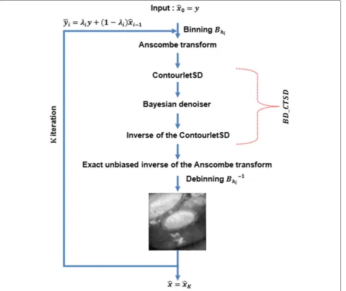
Figure9 resumes the steps of the proposed denoising algorithm.

In order to enhance the performance of our proposed denoiser, we follow the same steps as in the paper of Lucio Azzari and Alessandro Foi [7]. We use an iterative algorithm based on convex combination ofxi−1andy:

y_i=λiy+(1−λi)xi−1 (11)

where 0 < λ ≤ 1 andxi is the estimate ofx at

iter-ation i. λ depends on the number of iterations K and λK and is defined as λi = 1 − _Ki−₋1₁(1 − λK) where

the parameters K, λK are adaptively selected based on

enhancement of the results in terms of SNR neither of

CW by increasing the number of iterations. Furthermore,

the running time of the proposed algorithm increases. We usexi−1 instead of the previousxi, at each iteration of

the algorithm. We apply the Anscombe transformation

to image y_i, yielding fi = a(yi) = yATi. Then we

per-form a Bayesian denoising process BDCTSD to obtain a

denoised image Di = BDCTSD[a(yi)]. After gettingDi,

we return it to its original range by applying the exact unbiased inverse of fi [24]: We transform the image

y_i to the CTSD domain after applying the Anscombe transform,

xi=I_fλ_ii(Di) (12)

As in [7], we do the convex combination with a linear binning which can be especially beneficial at the first iterations.

xi=B−_hi1

Iλi

fi BDCTSD fi

Bhi[λi×y+(1−λi×xi−1)]

(13)

Bhiis the binning operator andhi is the size of the small

block atith iteration (i.e. binhi×hi). This operator can

be applied toy_i, yielding a smaller image where each bin ofhi×hi pixels fromyirepresents a single pixel equal to

their sum. Note thatBhi[yi] is subject to the same

condi-tional probability ofy_i which means that the adoption of binning does not interfere with the VST [7], neither with

BDCTSD[9].B−_hi1is the inverse binning operator. The entire

denoising algorithm is summarized in Fig.10.

Abbreviations

AT: Anscombe transformation; AWGN: Additive white Gaussian noise; CTSD: Transform with sharp frequency localization; DFB: Directional filter bank; EFTEM: Energy filter transmission electron microscopy; SNR: Signal-to-noise ratio; STD: Standard deviation; TET: Transmission electron tomography; VST: Variance stabilizing transformation

Acknowledgements

The authors wish to thank Sylvain Trépout for valuable discussions and suggestions concerning the biological data.

Funding

The project was supported by the High Ministry of Education of the Algerian Republic and Campus France, project 33257ZB, Huber Curien PHC Tassili, with grant number 15MDU950 and by Agence Nationale de la Recherche ANR-11-BSV8-016. The authors want to acknowledge the PICT-IBiSA for providing access to chemical imaging equipment. The funding bodies had no role in the design of the study and collection, analysis, and interpretation of data and in writing the manuscript.

Availability of data and materials

All data generated or analysed during this study are included in this published article and its supplementary information files.

Authors’ contributions

SSA, ZM and LB initiated the contribution. SSA implemented the algorithms in Matlab code and got the quantitative results. ZM and SM performed concept experiments and workflows. S.M and C.M performed EFTEM image

acquisitions. ZM, SM, LB, and AB coordinated the team. All authors contributed in drafting and reviewing the manuscript; also in analyzing, discussing and interpreting of the results. All authors read and approved the final manuscript.

Ethics approval and consent to participate

Not applicable.

Consent for publication

Not applicable.

Competing interests

The authors declare that they have no competing interests.

Publisher’s Note

Springer Nature remains neutral with regard to jurisdictional claims in published maps and institutional affiliations.

Author details

1_{Faculty of Science and Technology, Mohamed El Bachir El Ibrahimi University,}

Bordj Bou Arreridj, Algeria.2_{LIASD research Lab., Department of Computer}

Science, University of Paris 8, Saint-Denis, France.3_{Department of Computer}

and Information Sciences, Northumbria University, Newcastle upon Tyne, UK.

4_{INSERM, Institut Curie, University of Paris Saclay, Orsay, France.} Received: 5 October 2018 Accepted: 8 May 2019

References

1. Messaoudi C, Aschman N, Cunha M, Oikawa T, Sorzano CO, Marco S. Three-dimensional chemical mapping by eftem-tomoj including improvement of snr by pca and art reconstruction of volume by noise suppression. Microsc Microanal. 2013;19(6):1669–77.

2. Cunha ALD, Zhou J, Do MN. The nonsubsampled contourlet transform: theory, design, and applications. IEEE Trans Image Process. 2006;15(10): 3089–101.

3. Sid-Ahmed S, Messali Z, Ouahabi A, Trépout S, Messaoudi C, Marco S. Bilateral filtering and wavelets based image denoising: Application to electron microscopy images with low electron dose. Int J Recent Trends Eng Technol. 2014;11(1):153–64.

4. Zuo JM. Electron detection characteristics of a slow-scan ccd camera, imaging plates and film, and electron image restoration. Microsc Res Tech. 2000;49(3):245–68.

5. Vulovi´c M, Ravelli RB, van Vliet LJ, Koster AJ, Lazi´c LI, Lücken U, Rullgård H, Öktem O, Rieger B. Image formation modeling in cryo-electron microscopy. J Struct Biol. 2013;183(1):19–32.

6. Lu Y, Do MN. A new contourlet transform with sharp frequency localization. In: Proceedings of the 2006 IEEE International Conference on Image Processing (ICIP). Atlanta: IEEE; 2006. p. 1629–32.https://doi.org/ 10.1109/ICIP.2006.312657.

7. Azzari L, Foi A. Variance stabilization for noisy+estimate combination in iterative poisson denoising. IEEE Signal Process Lett. 2016;23(8):1086–90. 8. Boubchir L, Al-Maadeed S, Bouridane A. Undecimated wavelet-based

bayesian denoising in mixed poisson-gaussian noise with application on medical and biological images. In: The 4th International Conference on Image Processing Theory, Tools and Applications (IPTA). Paris: IEEE; 2014. p. 1–5.https://doi.org/10.1109/IPTA.2014.7001926.

9. Sid-Ahmed S, Messali Z, Ouahabi A, Trepout S, Messaoudi C, Sergio M. Nonparametric denoising methods based on contourlet transform with sharp frequency localization: Application to low exposure time electron microscopy images. Entropy. 2015;17(5):3461–78.

10. Boubchir L, Fadili J. A closed-form nonparametric bayesian estimator in the wavelet domain of images using an approximateα-stable prior. Pattern Recogn Lett. 2006;27(12):1370–82.

11. Boubchir L, Fadili J, Bloyet D. Bayesian denoising in the wavelet-domain using an analytical approximateα-stable prior. In: The 17th International Conference on Pattern Recognition (ICPR). Cambridge: IEEE; 2004. p. 889–92.https://doi.org/10.1109/ICPR.2004.1333915.

12. Boudjelal A, Messali Z, Boubchir L, Chetih N. Nonparametric bayesian estimation structures in the wavelet domain of multiple noisy image copies. In: The 6th International Conference on Sciences of Electronics, Technologies of Information and Telecommunications (SETIT). Sousse: IEEE; 2012. p. 495–501.https://doi.org/10.1109/SETIT.2012.6481962. 13. Sid-Ahmed S, Messali Z, Ouahabi A, Trepout S, Messaoudi C, Marco S,

Mohammad-Djafari A, Barbaresco F. Non parametric denoising methods based on wavelets: Application to electron microscopy images in low exposure time. In: AIP Conference Proceedings. AIP; 2015. p. 403–13. 14. Do MN, Vetterli M. The contourlet transform: an efficient directional

multiresolution image representation. IEEE Trans Image Process. 2005;14(12):2091–106.

15. Henderson R. Realizing the potential of electron cryo-microscopy. Q Rev Biophys. 2004;37(1):3–13.

16. Laurent G. Ecrans Plats et Vidéoprojecteurs - 2 Éd: Principes,

Fonctionnement et Maintenance. In: Audio-Photo-Vidéo. Dunod; 2014.

Conference on Image Processing (ICIP). Hong Kong: IEEE; 2010. p. 1877–80.https://doi.org/10.1109/ICIP.2010.5652329.

21. Boubchir L, Boashash B. Wavelet denoising based on the map estimation using the bkf prior with application to images and eeg signals. IEEE Trans Signal Process. 2013;61(8):1880–94.

22. Fadili J, Starck J-L, Boubchir L. Morphological diversity and sparse image denoising. IEEE Int Conf Acoust Speech Signal Process(ICASSP). 2007;I: 589–92.

23. H Sadreazami MOA, Swamy MNS. Contourlet domain image modeling by using the alpha-stable family of distributions. In: 2014 IEEE

International Symposium on Circuits and Systems (ISCAS). Melbourne VIC: IEEE; 2014.https://doi.org/10.1109/ISCAS.2014.6865378.