The Thirty-Third AAAI Conference on Artificial Intelligence (AAAI-19)
Automated Rule Base Completion as Bayesian Concept Induction
Zied Bouraoui
CRIL - CNRS & Univ Artois, France [email protected]
Steven Schockaert
Cardiff University, UK [email protected]Abstract
Considerable attention has recently been devoted to the prob-lem of automatically extending knowledge bases by applying some form of inductive reasoning. While the vast majority of existing work is centred around so-called knowledge graphs, in this paper we consider a setting where the input consists of a set of (existential) rules. To this end, we exploit a vec-tor space representation of the considered concepts, which is partly induced from the rule base itself and partly from a pre-trained word embedding. Inspired by recent approaches to concept induction, we then model rule templates in this vector space embedding using Gaussian distributions. Unlike many existing approaches, we learn rules by directly exploit-ing regularities in the given rule base, and do not require that a database with concept and relation instances is given. As a result, our method can be applied to a wide variety of on-tologies. We present experimental results that demonstrate the effectiveness of our method.
1
Introduction
The problem of automated knowledge base completion has received considerable attention in recent years (Pujara et al. 2017). Within the broad aim of knowledge base completion, various strategies can be explored. One possible strategy is to find missing facts by searching for relevant documents on the Web, and analyzing their content (West et al. 2014). Another strategy is to identify and exploit statistical regu-larities among the facts in a given knowledge base (Lao, Mitchell, and Cohen 2011; Bordes et al. 2013). Most ex-isting approaches, however, focus on finding plausible miss-ingfacts. Our focus in this paper is instead to find missing knowledge in a given ontology.
In particular, we propose an approach to find plausible rules which is inspired by cognitive models for category based induction (Osherson et al. 1990; Tenenbaum and Grif-fiths 2001). The main aim of such induction models is to de-termine which objects are likely to have some propertyP, knowing that the objects o1, ..., on have this property (but
knowing nothing else about property P). In other words, inductive generalization in these models is based on our knowledge of the semantic features of the objects. For ex-ample, knowing that oranges, lemons and grapefruit have
Copyright c2019, Association for the Advancement of Artificial Intelligence (www.aaai.org). All rights reserved.
some unknown property P, we can plausibly derive that limes have this property as well, simply because there are very few natural properties which hold for oranges, lemons and grapefruit, but not for lime. Similarly, suppose we have a knowledge base containing rules of the following form:
r1(X)∧orange(X)→r2(X)
r1(X)∧lemon(X)→r2(X)
r1(X)∧grapefruit(X)→r2(X)
Without knowing anything about the meaning of the rela-tionsr1 andr2, we can intuitively still derive that the
fol-lowing rule is plausible:
r1(X)∧lime(X)→r2(X)
To implement this intuition, we rely on two types of vector space representations of the considered relations. First, we can use word embeddings (Mikolov, Yih, and Zweig 2013; Pennington, Socher, and Manning 2014), which are vector space representations of word meaning that are learned from large text collections. Such representations have been found to exhibit various interesting regularities, which means that they can be regarded as a source of commonsense knowl-edge (Levy, Goldberg, and Ramat-Gan 2014; Gupta et al. 2015). Most importantly for our purposes, words represent-ing concepts with similar properties, such as different kinds of citrus fruits, tend to be clustered together. Second, we will also rely on a vector space representation that has been learned from the ontology itself. The aim of this represen-tation is to capture the intuition that relations which are as-serted to have similar properties should also be considered as similar for the purpose of inductive reasoning.
Similarly, by focusing on pairs of concepts, we can also complete rule bases using a form of analogical reasoning. Consider the following example:
r1(X, Y)∧bat(X)→cave(Y)
r1(X, Y)∧duck(X)→pond(Y)
r1(X, Y)∧dolphin(X)→sea(Y)
Then we can plausible also derive the following rule, based on the analogical relationship that holds between the pairs (bat,cave),(duck,pond),(dolphin,sea)and(trout,river):
Such analogical relationships can again be effectively iden-tified from word embeddings (Mikolov, Yih, and Zweig 2013), and other types of vector space representations.
To implement the aforementioned ideas for completing sets of rules, we will consider ruletemplates, such as
τ(?) =r1(X)∧?(X)→r2(X)
These templates are second-order relations, whose instances are the relations from the ontology. For example, the con-ceptsorange,lemonand grapefruit would be instances of the templateτ. This view will allow us to employ methods for concept and relation induction to predict plausible rules which are missing from a given ontology.
2
Related Work
Within the area of knowledge base completion, we can iden-tify three classes of related work.
Methods for completing ABoxes and knowledge graphs.
This class of methods focuses on finding missing facts. For example, a number of methods have been proposed that learn latent soft clusters of predicates to predict missing facts in relational data (Kok and Domingos 2007; Rockt¨aschel and Riedel 2016; Sourek et al. 2016). Within the area of knowledge graph completion, the most popular strategies are based on embedding relations and entities in a low-dimensional vector space, e.g. by modelling binary relations as vector translations (Bordes et al. 2013), or on identify-ing types of paths in the knowledge graph which are predic-tive of a given relationship (Gardner et al. 2014). Another possible strategy to find missing facts consists in extracting them from natural language statements (Mintz et al. 2009; Riedel, Yao, and McCallum 2010; West et al. 2014). Most relevant for our work, some authors have also looked at pre-dicting missing facts by modelling concepts in some under-lying feature space. For example, Neelakantan and Chang (2015) represent each Freebase entity using a combination of features derived from Freebase itself and from Wikipedia, and then use a max-margin model to identify missing types. In (Bouraoui, Jameel, and Schockaert 2017), description logic concepts were modelled as Gaussians in a vector space embedding.
Methods for learning rules from instances.In this paper, our focus is on predicting rules without using any database of facts (e.g. ABox assertions), which is motivated by the fact that for many useful ontologies no such database is available. However, when a sufficiently large database of facts is given, methods from Inductive Logic Programming (B¨uhmann, Lehmann, and Westphal 2016), or based on For-mal Concept Analysis (Baader et al. 2007) or Association Rule Mining (V¨olker and Niepert 2011), can be used to con-struct plausible rules. Such rules make explicit some of the regularities that are observed among the given facts, beyond those which are already encoded in the ontology.
Methods for completing rule bases.The problem of pre-dicting plausible missing rules for a given rule base has not yet received much attention. In (Schockaert and Prade 2013), methods for completing propositional rule bases have
been proposed, based on interpolation and analogical rea-soning, but they were only studied from a theoretical point of view. Moreover, the methods proposed there require back-ground knowledge, such as a betweenness relation in the case of interpolation, which is not readily available. In this paper, we avoid this issue by relying on word embeddings.
The idea of similarity based reasoning, as a general strat-egy for extending (the applicability of) rule bases, has been explored in a number of ways. For example, (Beltagy et al. 2013) uses Markov logic to consider defeasible rules of the formcucumber(X)→zucchini(X), to encode the intuition that many rules about cucumbers also apply to zucchinis. Conceptually this achieves a kind of similarity-based rule base completion (e.g. we may imagine adding a rule about zucchinis for each rule we have about cucumbers), although the extended knowledge base is not explicitly constructed.
Along similar lines, there have been a few proposals to extend logic programming with a soft unification mecha-nism, where a given rule is triggered, to some degree, if a formula is satisfied which is similar to the body of that rule, either based on a given similarity structure (Medina, Ojeda-Aciego, and Vojt´aˇs 2004) or by similarity degrees which are induced from a vector space embedding (Rockt¨aschel and Riedel 2017).
3
Background
Ontologies express structured knowledge about the con-cepts, properties and relations of a given domain. Descrip-tion logics and existential rules are the two main logical frameworks underlying ontology languages. While descrip-tion logics are most often used in practice, in this paper we will consider existential rules, as this will simplify the pre-sentation. Note however that the method we present in this paper could be straightforwardly applied to description logic axioms as well. Here we briefly recall the syntax of existen-tial rules; for a comprehensive overview of this framework we refer to (Baget et al. 2011).
The syntax of existential rules is defined over a vocabu-lary of a finite set of relations (i.e. predicates) and an infinite set of constants. Anexistential ruleis a first-order rule of the following form:
r1(x1)∧...∧rn(xn)→ ∃y. s1(z1)∧...∧sm(zm) (1) Herex1, ...,xn,y,z1, ...,zmare tuples of variables and for each i ∈ {1, ..., m}we have vars(zi) ⊆ vars(x1)∪...∪ vars(xn)∪ vars(y), where we write vars(x) for the set of variables appearing in the tuple x. An example of ex-istential rule is sibling(x1, x2) → ∃y. parentOf(y, x1)∧
parentOf(y, x2)wheresiblingandparentOf are predicates
andx1,x2andyare variables. Note that the tupleymay be
empty, which means that rules without an existential quanti-fier (e.g.sibling(x1, x2)→sibling(x2, x1)) are also special
set of existential rules, which are usually assumed to be non-fact rules. The variables in an existential rule are implicitly assumed to be universally quantified. Standard notions such as consistency and entailment are then defined in the usual way.
4
A Model for Rule Induction
Throughout this section, we let R be a set of existential rules. The problem we consider is to identify rulesρwhich are not entailed byR, but are nonetheless plausible. As al-ready mentioned in the introduction, our strategy is to con-sider rule templates, and to characterize the kind of relations that fit these templates based on vector space representations of these relations. In Section 4.1, we first explain what kind of templates are considered. Subsequently, in Section 4.2, we discuss in more detail how vector space representations can be used to represent relations. Then Sections 4.3 and 4.4 explain our induction models, respectively for unary and for binary templates. Finally, Section 4.5 discusses our overall approach to making predictions.
4.1
Rule Templates
We will consider two kinds of templates, which respectively replace one and two occurrences of relations by a second-order variable. Specifically, letρbe an existential rule of the form (1). Thenρinduces the following unary templates:
?(x1)∧...∧rn(xn)→ ∃y. s1(z1)∧...∧sm(zm) ...
r1(x1)∧...∧rn(xn)→ ∃y. s1(z1)∧...∧?(zm)
We will write τ(?), or simply τ, to denote a given unary template, whereτ(r)then corresponds to the rule that is ob-tained when instantiating the second-order variable? with the relationr. Let us furthermore writeT1(ρ)for the set of
all unary templates that can be obtained from the ruleρ, and letT1(R) =Sρ∈RT1(ρ). Similarly, the ruleρinduces the
following binary templates:
?(x1)∧ •(x2)∧...∧rn(xn)→ ∃y.s1(z1)∧...∧sm(zm) ...
?(x1)∧...∧rn(xn)→ ∃y.s1(z1)∧...∧ •(zm) ...
r1(x1)∧...∧rn(xn)→ ∃y.s1(z1)∧...∧?(zm−1)∧ •(zm)
where?and• are second-order variables. We writeT2(ρ)
for the set of all binary templates that can be obtained from ρandT2(R) =Sρ∈RT2(ρ). Similar as for unary templates,
we writeτ(?,•)to refer to a template, andτ(r, s)to the rule that is obtained by instantiating the second-order variables? and•byrandsrespectively.
For a given unary templateτ, we writeπ(R, τ)for the set of relations that satisfy the templates inR, i.e.:
r∈π(R, τ)⇔τ(r)∈ R
Note that all relations inπ(R, τ)will have the same arity, which we will also refer to as the arity of the template τ.
Similarly, for a binary templateτ,π(R, τ)represents the set of relation pairs that lead to a rule fromR, i.e.:
(r, s)∈π(R, τ)⇔τ(r, s)∈ R
We now illustrate these notions in the following example.
Example 1. Let us consider the following set of rulesR:
livesIn(X, Y)∧bat(X)→cave(Y) livesIn(X, Y)∧duck(X)→pond(Y)
ThenT1(R)contains the following unary templates:
τ1(?) = ?(X, Y)∧bat(X)→cave(Y)
τ2(?) = ?(X, Y)∧dolphin(X)→sea(Y)
τ3(?) = livesIn(X, Y)∧?(X)→cave(Y)
τ4(?) = livesIn(X, Y)∧bat(X)→?(Y)
τ5(?) = livesIn(X, Y)∧?(X)→pond(Y)
τ6(?) = livesIn(X, Y)∧duck(X)→?(Y)
whileT2(R)contains the following binary templates:
τ7(?,•) = ?(X, Y)∧ •(X)→cave(Y)
τ8(?,•) = ?(X, Y)∧ •(X)→pond(Y)
τ9(?,•) = ?(X, Y)∧bat(X)→ •(Y)
τ10(?,•) = ?(X, Y)∧duck(X)→ •(Y)
τ11(?,•) = livesIn(X, Y)∧?(X)→ •(Y)
Then we have e.g.:
π(R, τ1) ={livesIn}
π(R, τ7) ={(livesIn,bat)}
π(R, τ11) ={(bat,cave),(duck,pond)}
Our approach will be based on characterizing the com-monalities of the relations in π(R, τ). However, in some cases the templates we obtain might be too general for such characterizations to be meaningful. A typical example are subsumption rules such as orange(X) → citrusFruit(X), which gives rise to the binary templateτ(?,•) = ?(X)→ •(X). The instances of this template may have little or noth-ing in common, hence it would not be effective as a basis for induction. Therefore, we will also consider two kinds of restricted templates.
First, we considertyped rule templates, in which the pos-sible instantiations of the second-order variables are limited to relations that are subsumed by a given relation. Letτ(?,•) be a binary template, and letrandsbe two relations. Then τ(?↓r,•↓s)is a typed template, whose instances are defined
as follows: we have(r0, s0)∈π(R, τ(?↓r,•↓s))if the
fol-lowing three conditions are satisfied:
1. (r0, s0)∈π(R, τ(?,•))
2. R |=r0(X1, ..., Xk)→r(X1, ..., Xk)
3. R |=s0(X1, ..., Xl)→s(X1, ..., Xl)
suffix or prefix often have something in common (e.g. rugby-Player,tennisPlayer,baseballPlayer). If a naming conven-tion is used which allows us to easily split relaconven-tion names into meaningful constituents, we can easily restrict tem-plates to relations that have a name with a particular suf-fix or presuf-fix. In particular, we writeτ(?−str1,•−str2)for the name-constrained restriction ofτ(?,•)in which?can only be instantiated by relations whose name ends withstr1and•
can only be instantiated by relations whose name ends with str2, and similar for prefixes.
4.2
Vector Space Representations
Given a templateτ, and the knowledge thatτ(r1), ..., τ(rn)
are valid rules, the main inference task we consider is to identify relations sfor whichτ(s)is a plausible rule, and similar for binary templates. To this end, we will use two types of vector space representations.
Word embeddings. First, we will use a pre-trained word embedding. Word embeddings allow us to exploit lexical background knowledge, intuitively enabling us to make pre-dictions based on the idea that relations with similar names tend to have similar properties. To this end, we first tok-enize the relation name using a small set of simple heuris-tics, based on standard ontology naming conventions. For instance,ProfessionalRugbyPlayerwould be converted into a list of three words:professional,rugbyandplayer. A rela-tionrcorresponding to the list of wordsw1, ..., wn is then
represented as the vectorvw
r = n1(w1+...+wn), where
we writewifor the vector representation of wordwi in the
word embedding. While simply averaging the word vectors might seem naive, this strategy is known to be surprisingly effective for short texts (Hill, Cho, and Korhonen 2016).
Matrix factorization for unary templates.In addition to using the relation names, we can also derive information about the similarity of relations from the given rule base it-self. Here the intuition is that relations which already ap-pear in similar rules from the rule base should be consid-ered to be similar. To implement this intuition, we will ap-ply the idea from the AnalogySpace model (Speer, Havasi, and Lieberman 2008). The aim of that model is to learn low-dimensional vector space representation of the concepts in the ConceptNet knowledge graph, by factorizing a ma-trix whose rows are concepts and whose columns are prop-erties of these concepts. Adapted to our context, we start with a matrixM1whose rows are the unary templates from T1(R), possibly extended by some of their typed or
name-constrained variants. For efficiency reasons, we only include those templatesτfor which|π(R, τ)| ≥2. The columns of M1 correspond to the relations fromR. There is a 1 in the
row forτ and column forriffr∈ π(R, τ), and a 0 other-wise.
The AnalogySpace method is based on the Singular Value Decomposition (SVD) ofM1 = UΣVT. In particular, the
diagonal matrixΣis replaced by the matrix Σk, in which
all but the firstkdiagonal elements are replaced by0. Using Σk, we can compute the approximation1M10 =UΣkVT of
1
A well-known property of SVD is thatM10is the rank-kmatrix which is most similar toM1, in terms of the Frobenius norm.
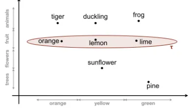
Figure 1: Modelling templates as ellipsoidal regions.
the matrixM1. Entries inM10which are close to 1, but which
were 0 inM1then correspond to plausible rules which are
missing fromR, i.e. if the entry on the row of templateτand the column of relationris close to 1, then we may conclude that τ(r)is a plausible rule. This strategy was empirically found to work well in (Speer, Havasi, and Lieberman 2008) for finding plausible missing links in ConceptNet, but has not yet been considered for finding plausible rules. We will evaluate this strategy as one of our baselines in Section 5.
In our model, we will use the SVD decomposition ofM1
in another way. In particular, we can use Principal Compo-nent Analysis (PCA) to obtain a low-dimensional represen-tation of the relations which maximally preserves the infor-mation encoded in M1. To this end, we represent each
re-lation ras the k-dimensional vector which is obtained by taking the firstkcolumns of the row corresponding torin the matrixVΣ. Let us denote thisk-dimensional vector by vrR. In our model, we will use the vectorsvrwandvrRas two
alternative representations of the relationr.
Matrix factorization for binary templates. We can also obtain a vector space representation of relation pairs, by ap-plying PCA to the matrix M2, whose rows are the binary
templates (with at least two instances) and whose columns are relation pairs (which are instances of at least one tem-plate). Let us writeuRr,sfor the resultingk-dimensional vec-tor representation of the relation pair (r, s). Similar as for unary templates, we will also use SVD to obtain a rank-k approximation of the matrixM2as a baseline strategy.
4.3
Unary Template Model
Intuition. Let us write vr for the vector space
represen-tation of relation r (i.e. one of the two types of represen-tations discussed in Section 4.2). Our main assumption is that the relations which satisfy some template τ are clus-tered together in the vector space. Whether this assumption is reasonable (for a given type of vector space) is an empiri-cal question, which we will attempt to answer in our experi-mental evaluation below. However, a similar assumption was found to lead to good performance in (Bouraoui, Jameel, and Schockaert 2017) for the task of ABox completion.
The most straightforward way to implement this assump-tion would be to learn a vector vτ for the given template,
and vr. This closely corresponds to the strategy that was
adopted in (Rockt¨aschel and Riedel 2017), although in a dif-ferent setting. Note that the representation of a template in the vector space can then be viewed as a sequence of con-centric spheres, containing the vectors of increasingly less similar relations. However, this relies on the rather unre-alistic assumption that all dimensions of the vector space are equally important. For example, it was found in (Mu, Bhat, and Viswanath 2017) that some dimensions in pop-ular word embedding models are far less informative than others. More generally, what typically matters is whether re-lations are similar with respect to particular facets. For ex-ample,lemonandlimeare similar in most respects, but they have a different color. Accordingly, in some contexts, we may actually have to consider thatlimeis more similar to frog (because they are both green) than tolemon. To take this context-dependent nature of similarity into account, we will model templates using ellipsoidal regions in the vector space, instead of spheres. To illustrate this, Figure 1 shows a toy example with one dimension along which concepts are organized by color and one dimension along which con-cepts are organized by type. When modelling the template ?(X)→ fruit(X), only the latter really matters, leading to the ellipse shown in the figure.
To find a suitable (soft) ellipsoidal region for a given unary templateτ, we will estimate a Gaussian distribution from the vector representations of the relations inπ(R, τ). This allows us to use the standard Bayesian machinery for estimating Gaussians, based on conjugate priors, which of-fers a convenient and principled way of avoiding overfit-ting. Conceptually, the resulting method for predicting plau-sible rules can be seen as the implementation of a form of commonsense reasoning which is known as interpolation (Schockaert and Prade 2013). In particular, the Gaussian modelling the templateτ will offer us a convenient way of deciding whether a given relationris sufficiently “between” the relations which are known to satisfyτ, to plausibly con-clude thatrsatisfiesτas well.
Model description.Our aim is to evaluate the probability that a given templateτ satisfies a relationr, knowing that it satisfies the relationsr1, ..., rn. Using Bayes’ rule we can
express this as follows:
P(τ(r)|vr) =λτ·
f(vr|τ(r))
f(vr)
(2)
Heref(.|τ(r))is a Gaussian distribution modelling the re-lations satisfying the templateτ. This distribution will be estimated from the vector representations of the relations r1, ..., rn. The distributionf(.)expresses how likely the
vec-tor representationvritself is. It will be estimated as a
Gaus-sian from the vector representations of the overall set of re-lations. In case the templateτ is typed, however,f(vr)is
estimated from the relations that have the correct type only, and similar for name-constrained templates. Finally,λτ is
the prior probability that a given relation satisfies the tem-plate. It will act as a scaling factor.
Estimating Gaussians.Sincef(.|τ(r))typically has to be modelled from a very small number of examples, we need to
make some drastic regularity assumptions. In particular, we will make the common assumption that this Gaussian distri-bution has a diagonal covariance matrix (Vilnis and McCal-lum 2015). This means that we can evaluate this probability using a product of univariate Gaussians:
f(vr|τ(r)) = m
Y
i=1
G(xri;µi, σi2)
wheremis the number of dimensions in the vector space and we writexri for theithcoordinate ofv
r. To estimate the
pa-rametersµiandσ2i of these univariate Gaussians, we follow
a Bayesian approach, i.e. rather than taking a single estimate, we take a weighted average based on a probability distribu-tion over plausible values for these parameters. Compared to using maximum likelihood estimates, Bayesian estima-tion is more cautious and less prone to overfitting. A par-ticular consequence is that templates with few instances are penalized, which will help our method to focus on the most reliable templates. Formally, the probabilityG(xri;µi, σ2i)is
then estimated as:
Z
G(xri;µ, σ2)NIχ2(µ, σ2|µ0, κ0, ν0, σ20)dµdσ
whereNIχ2is the normal inverseχ2 distribution, which is
the standard conjugate prior of the Gaussian distribution. It encodes which values of the parametersµandσ2are likely,
given that theith coordinate of the vectorsv
1, ..., vn is
as-sumed to have been generated from that distribution, and possibly some prior information. In our setting, we will not assume that any prior information is given, in which case a flat prior can be used. It can be shown that the integral then evaluates to (Murphy 2007):
tn−1
xi,
(n+ 1)Pn
j=1(x
rj
i −xi)2
n(n−1)
where xi = 1nP n j=1x
rj
i and tn−1 is the Student
t-distribution withn−1degrees of freedom. We refer to (Mur-phy 2007) for more details on the Bayesian estimation of Gaussian distributions. The probability f(vr)is estimated
in the same way, but based on the set of all relations (of the considered type), rather than only those inπ(R, τ).
Estimating the prior.The priorλτ is estimated by
maxi-mizing the log-likelihood of the rules inR. Let the arity of the templateτ bea, and letRabe the set of all relations of
aritya. We then choose the value ofλτ that maximizes:
X
r∈π(R,τ)
logP(τ(r)|vr) +
X
r∈Ra\π(R,τ)
log(1−P(τ(r)|vr))
whereP(τ|vr), for a given choice ofλτ, is evaluated as in
(2). Note that this estimation ofλτ relies on a closed world
does not apply). As a consequence, the value ofλτ may be
lower than it should be. However, this is typically not a prob-lem, as it simply means that the predictions we make might be more cautious then they need to be. As a second simplifi-cation, in the case of large rule bases, the second summation will be restricted to a sample ofRa\π(R, τ)for
computa-tional reasons. A close approximation to this summation can be obtained by selecting the elements fromRa \ π(R, τ)
whose vector representation is closest to the mean of the Gaussianf(.|τ(r))(e.g. using a k-d tree).
4.4
Binary Template Model
Intuition. Like the unary templates, binary templates will also be modelled using Gaussian distributions. In the case of binary templates, however, there will be several Gaussians that are used in combination. In particular, we will learn (i) a Gaussian to model the kind of relations that may instanti-ate?(ii) a Gaussian to model the kind of relations that many instantiate•, (iii) a Gaussian over the set of vector transla-tionsvs−vr of valid instances(r, s)of the template, and,
in case the SVD based vector representations are used, (iv) a Gaussian in the vector space of relation pairs. A model based on (i)–(iii) was already found to perform well for the task of relation induction in (Bouraoui, Jameel, and Schock-aert 2018), but it will here be adapted for the task of rule induction.
Model description.The probabilityP(τ(r, s)|vr, vs, ur,s)
that a relation pair (r, s)satisfies the binary templateτ is estimated as follows:
λτ·
f(vr|τ(r,•))
f(vr)
·f(vs|τ(?, s))
f(vs)
· f(vs−vr|τ(r, s))
f(vs−vr|τ(r,•), τ(?, s))
·f(ur,s|τ(r, s))
The scaling parameterλτ and the probabilities f(vr)and
f(vs)are estimated similarly as in the unary template model.
The probabilityf(vr|τ(r,•))represents how likely the
vec-tor representation vr is, given that there exists some
rela-tiont such thatτ(r, t)is a valid rule. It is estimated simi-larly to how we estimatedf(vr|τ(r))in the unary template
model. The probabilityf(vs|τ(?, s))is also estimated in a
similar way, but based on the second arguments of the ele-ments inπ(R, τ). The probabilityf(vs−vr|τ(r, s))is again
estimated similarly, but now based on the vector differences vs1 −vr1 of the elements (r1, s1)of π(R, τ). Finally, the probabilityf(vs −vr|τ(r,•), τ(?, s)) is estimated as
fol-lows. Let A = {r1, ..., rk} andB = {s1, ..., sl}
respec-tively be the relations that occur as a first and as a second argument in the elements ofπ(R, τ). Eachriis paired with
a randomly selected elements0i fromB. Then we estimate f(vs−vr|τ(r,•), τ(?, s))like f(vs −vr|τ(r, s)), but by
using the vector differencess0
1−r1, ..., s0k−rkinstead.
Note that the vectorsur,s are only available when using
the vector representations obtained by PCA. In the variant of this model where we use vectors from word embeddings instead, the factorf(ur,s|τ(r, s))is simply dropped.
4.5
Making Predictions
To estimate the probability that a ruleρis valid, we first de-termine the corresponding set of unary templates T1(ρ) = {τ1, ..., τk} and binary templates T2(ρ) = {τk+1, ..., τl}.
For each unary templateτi letri be the relation for which
ρ =τi(yi),1 ≤ i ≤k. Similarly, for a binary templateτi
we writeρ=τi(ri, si),k+ 1≤i≤l. The overall
probabil-ity is then obtained by aggregating the probabilities obtained from both vector space representations, for each template, and then maximizing the resulting probabilities:
P(ρ| R) = max max
1≤i≤kP(τi(ri)|v
w
ri, v
R
ri),
max
k+1≤i≤lP(τi(ri, si)|v
w
ri, v w
si, v
R
ri, v
R
si, u
R
ri,si)
whereP(τi(ri)|vrwi, v
R
ri)is evaluated as:
µP(τi(ri)|vrRi) + (1−µ)P(τi(ri)|v w
ri)
withµ ∈ [0,1]a parameter controlling the relative impor-tance of the two types of vector space representations. Sim-ilarlyP(τi(ri, si)|vwri, v
w
si, v
R
ri, v
R
si, u
R
ri,si)is evaluated as:
µP(τi(ri, si)|vrRi, v
R
si, u
R
ri,si) + (1−µ)P(τi(ri, si)|v w
ri, v w
si)
5
Experimental Results
In this section, we experimentally analyze the performance of our method. As knowledge bases we consider several well-known OWLontologies, which we converted to exis-tential rule bases. In particular, we consider two large-scale open-domain ontologies: SUMO and OpenCyc. We also test the performance on a number of smaller domain-specific on-tologies: Wine ontology, Economy, Transport and Vicodi. Before converting each OWL ontology to a rule base R, we use the pellet reasoner to compute the set of inferred axioms (subclasses, equivalent classes, sub-object proper-ties and equivalent object properproper-ties), and we add the corre-sponding rules toRas well. As word embedding, We used a standard pre-trained 300-dimensional, which was learned using Skip-gram on the 100B words Google News corpus.
To evaluate the performance of different methods, we split the considered rule base into training and test sets. After splitting the rule base, we remove from the test set all rules that can be deduced from the training set. To evaluate our model, we will also need negative examples, in addition to the positive examples from the test set. Following a com-mon practice in the context of knowledge base completion, we will generate a number of synthetic negative examples, which we will call distractor rules. In particular, following the strategy used in (Vylomova et al. 2016) for evaluating relation induction models, for each correct test rulebody→
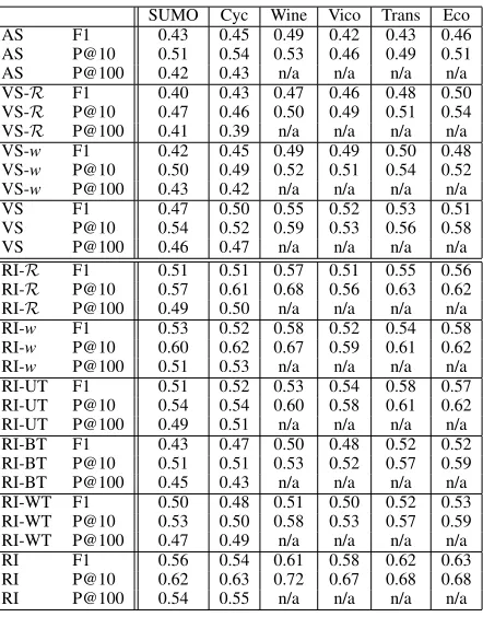
Table 1: Overview of experimental results.
SUMO Cyc Wine Vico Trans Eco AS F1 0.43 0.45 0.49 0.42 0.43 0.46 AS P@10 0.51 0.54 0.53 0.46 0.49 0.51 AS P@100 0.42 0.43 n/a n/a n/a n/a VS-R F1 0.40 0.43 0.47 0.46 0.48 0.50 VS-R P@10 0.47 0.46 0.50 0.49 0.51 0.54 VS-R P@100 0.41 0.39 n/a n/a n/a n/a VS-w F1 0.42 0.45 0.49 0.49 0.50 0.48 VS-w P@10 0.50 0.49 0.52 0.51 0.54 0.52 VS-w P@100 0.43 0.42 n/a n/a n/a n/a VS F1 0.47 0.50 0.55 0.52 0.53 0.51 VS P@10 0.54 0.52 0.59 0.53 0.56 0.58 VS P@100 0.46 0.47 n/a n/a n/a n/a RI-R F1 0.51 0.51 0.57 0.51 0.55 0.56 RI-R P@10 0.57 0.61 0.68 0.56 0.63 0.62 RI-R P@100 0.49 0.50 n/a n/a n/a n/a RI-w F1 0.53 0.52 0.58 0.52 0.54 0.58 RI-w P@10 0.60 0.62 0.67 0.59 0.61 0.62 RI-w P@100 0.51 0.53 n/a n/a n/a n/a RI-UT F1 0.51 0.52 0.53 0.54 0.58 0.57 RI-UT P@10 0.54 0.54 0.60 0.58 0.61 0.62 RI-UT P@100 0.49 0.51 n/a n/a n/a n/a RI-BT F1 0.43 0.47 0.50 0.48 0.52 0.52 RI-BT P@10 0.51 0.51 0.53 0.52 0.57 0.59 RI-BT P@100 0.45 0.43 n/a n/a n/a n/a RI-WT F1 0.50 0.48 0.51 0.50 0.52 0.53 RI-WT P@10 0.53 0.50 0.58 0.53 0.57 0.59 RI-WT P@100 0.47 0.49 n/a n/a n/a n/a RI F1 0.56 0.54 0.61 0.58 0.62 0.63 RI P@10 0.62 0.63 0.72 0.67 0.68 0.68 RI P@100 0.54 0.55 n/a n/a n/a n/a
vast majority of them. To split the rule bases into training and test rules, we use 10-fold cross validation.
The considered task can be evaluated as a ranking task or as a classification task. When we consider it as a rank-ing task, the aim is to rank the correct test rules higher than the distractor rules. To evaluate the quality of the rankings produced by the different methods, we use precision at n (P@n), which is simply the percentage of the n highest ranked rules that correspond to correct test rules. We can also consider a classification task, i.e. for each rule in the test data decide whether it is a correct test rule or a distrac-tor, where we report the F1 score.
To set the parameters of our model (and the baselines), we select 10% of the training data as validation data, and only use the remaining 90% for training the model. This valida-tion data is used for selecting the parameterµand for choos-ing the number of dimensions in the vector space representa-tionsvRr (chosen from{10,25,50,100}). For the classifica-tion experiments, we also tune a threshold on the probability for a rule to be predicted as valid.
In the following we will refer to our model asRI(for Rule Induction). To better understand the impact of each com-ponent, we will also consider the following variants:RI-R
only uses the vector representations obtained using PCA and
RI-wonly uses vector representations from the word embed-ding, RI-UT only uses unary templates,RI-BT only uses binary templates, and RI-WT is our full model but with-out using restricted templates. We will also show results for two baselines. First, we will use the AnalogySpace model applied to unary rule templates, as described in Section 4.2 (AS). When used in a classification setting, we tune a
thresh-old on the values of entries fromM10 above which the
cor-responding rule is considered valid. Second, we will use a similarity based model (VS). Given a templateτ, we then learn a template vectorvτ which is the average of the
vec-tors of the relations that satisfy this template, and then we tune a threshold on the similarity between this vector and the relation vectors to make predictions. To make the results comparable to those forRI, we represent each relation using the concatenation of its representation from the word em-bedding and from the PCA space. We also consider the vari-antsVS-RandVS-w, which respectively only use the PCA space and the word embedding. This baseline will allow us to assess the benefit of using elliptical rather than spherical regions for characterizing templates.
An overview of the experimental results is presented in Table 1; note that no P@100 results are shown for the smaller ontologies, as the number of test rules is less than 100 in these cases. A number of conclusions can be drawn from the results. First, the proposed model clearly and con-sistently outperforms the baselines. Second, the PCA vec-tor space and the word embedding space perform similarly, when used in isolation, but using the full model offers sub-stantial further improvements. This illustrates the fact that both spaces effectively capture complementary information. Third, the RI-UT and RI-BT both perform clearly worse than the full model, showing that both types of templates are indeed necessary to achieve optimal results. Finally, the relatively poor performance ofRI-WT is largely due the fact that most of the binary templates are very general, and there-fore only become informative when we restrict them in a suitable way.
To illustrate how our model can outperform the similarity based strategy of VS, we give examples of rules that our model was able to predict, which go beyond similarity based reasoning. From the SUMO ontology, for instance, the unary template model correctly2predicts:
Pipeline(X)→Transitway(X)
The template τ1(?) = ?(X)→Transitway(X) was
used to predict this rule, with π(R, τ1) = {Airway,
LandTransitway,Waterway,AirTransitway}. Another exam-ple is the ruleSand(X) → Soil(X) which was predicted fromτ2(?) =?(X)→Soil(X)andπ(R, τ2) ={Loam,Silt,
Clay}.
6
Conclusions
We have proposed a method for predicting plausible miss-ing rules from a given ontology (i.e. a set of existential rules). The main underlying idea is to consider rule tem-plates, which are second-order predicates whose instances correspond to rules. These templates allow us to approach the considered problem of rule induction as a particular kind of concept or relation induction problem. By considering both unary and binary rule templates, our method is able to implement several well-known commonsense reasoning
2
strategies, including interpolation, similarity-based reason-ing and analogical reasonreason-ing. From an application point of view, our method is easy to use, as the only required input is a rule base and a standard pre-trained word embedding.
Acknowledgments
Steven Schockaert was supported by ERC Starting Grant 637277.
References
Baader, F.; Ganter, B.; Sertkaya, B.; and Sattler, U. 2007. Completing description logic knowledge bases using formal concept analysis. InProc. IJCAI, volume 7, 230–235. Baget, J.; Lecl`ere, M.; Mugnier, M.; and Salvat, E. 2011. On rules with existential variables: Walking the decidability line. Artif. Intell.175(9-10):1620–1654.
Beltagy, I.; Chau, C.; Boleda, G.; Garrette, D.; Erk, K.; and Mooney, R. 2013. Montague meets Markov: Deep se-mantics with probabilistic logical form. InProceedings of *SEM13, 11–21.
Bordes, A.; Usunier, N.; Garcia-Duran, A.; Weston, J.; and Yakhnenko, O. 2013. Translating embeddings for modeling multi-relational data. InProc. NIPS. 2787–2795.
Bouraoui, Z.; Jameel, S.; and Schockaert, S. 2017. Induc-tive reasoning about ontologies using conceptual spaces. In Proc. AAAI, 4364–4370.
Bouraoui, Z.; Jameel, S.; and Schockaert, S. 2018. Relation induction in word embeddings revisited. InProc. COLING. B¨uhmann, L.; Lehmann, J.; and Westphal, P. 2016. Dl-learner–a framework for inductive learning on the semantic web.Journal of Web Semantics39:15–24.
Gardner, M.; Talukdar, P.; Krishnamurthy, J.; and Mitchell, T. 2014. Incorporating vector space similarity in random walk inference over knowledge bases. In Proc. EMNLP, 397–406.
Gupta, A.; Boleda, G.; Baroni, M.; and Pad´o, S. 2015. Dis-tributional vectors encode referential attributes. In Proc. EMNLP, 12–21.
Hill, F.; Cho, K.; and Korhonen, A. 2016. Learning dis-tributed representations of sentences from unlabelled data. InProc. NAACL-HLT, 1367–1377.
Kok, S., and Domingos, P. 2007. Statistical predicate inven-tion. InProc. ICML, 433–440.
Lao, N.; Mitchell, T.; and Cohen, W. W. 2011. Random walk inference and learning in a large scale knowledge base. In Proceedings of EMNLP, 529–539.
Levy, O.; Goldberg, Y.; and Ramat-Gan, I. 2014. Linguistic regularities in sparse and explicit word representations. In Proc. CoNLL, 171–180.
Medina, J.; Ojeda-Aciego, M.; and Vojt´aˇs, P. 2004. Similarity-based unification: a multi-adjoint approach. Fuzzy sets and systems146:43–62.
Mikolov, T.; Yih, W.-t.; and Zweig, G. 2013. Linguistic reg-ularities in continuous space word representations. InProc. NAACL-HLT, 746–751.
Mintz, M.; Bills, S.; Snow, R.; and Jurafsky, D. 2009. Dis-tant supervision for relation extraction without labeled data. InProc. ACL, 1003–1011.
Mu, J.; Bhat, S.; and Viswanath, P. 2017. All-but-the-top: Simple and effective postprocessing for word representa-tions.CoRRabs/1702.01417.
Murphy, K. 2007. Conjugate Bayesian analysis of the Gaus-sian distribution. Technical report, University of British Columbia.
Neelakantan, A., and Chang, M. 2015. Inferring missing entity type instances for knowledge base completion: New dataset and methods. InProc. NAACL, 515–525.
Osherson, D. N.; Smith, E. E.; Wilkie, O.; Lopez, A.; and Shafir, E. 1990. Category-based induction. Psychological review97(2):185–200.
Pennington, J.; Socher, R.; and Manning, C. D. 2014. Glove: Global vectors for word representation. InEMNLP, 1532– 1543.
Pujara, J.; Chen, D.; Dalvi, B.; and Rockt¨aschel, S. S. T., eds. 2017. Proc. Workshop on Automated Knowledge Base Construction.
Riedel, S.; Yao, L.; and McCallum, A. 2010. Modeling relations and their mentions without labeled text. InProc. ECML/PKDD, 148–163.
Rockt¨aschel, T., and Riedel, S. 2016. Learning knowledge base inference with neural theorem provers. InProceedings of the 5th Workshop on Automated Knowledge Base Con-struction, 45–50.
Rockt¨aschel, T., and Riedel, S. 2017. End-to-end differen-tiable proving. InProc. NIPS, 3791–3803.
Schockaert, S., and Prade, H. 2013. Interpolative and ex-trapolative reasoning in propositional theories using qualita-tive knowledge about conceptual spaces.Artif.Intell202:86– 131.
Sourek, G.; Manandhar, S.; Zelezn´y, F.; Schockaert, S.; and Kuzelka, O. 2016. Learning predictive categories using lifted relational neural networks. InProc. ILP, 108–119. Speer, R.; Havasi, C.; and Lieberman, H. 2008. Analogys-pace: reducing the dimensionality of common sense knowl-edge. InProc. AAAI, 548–553.
Tenenbaum, J. B., and Griffiths, T. L. 2001. Generalization, similarity, and bayesian inference. Behavioral and Brain Sciences24:629–640.
Vilnis, L., and McCallum, A. 2015. Word representations via gaussian embedding. InProceedings of the International Conference on Learning Representations.
V¨olker, J., and Niepert, M. 2011. Statistical schema induc-tion. InProc. ESWC, 124–138.
Vylomova, E.; Rimell, L.; Cohn, T.; and Baldwin, T. 2016. Take and took, gaggle and goose, book and read: Evaluating the utility of vector differences for lexical relation learning. InProc. ACL.