Quantifying skull shape

(1)

MURDOCH RESEARCH REPOSITORY

http://dx.doi.org/10.1109/ICARCV.2002.1234881

Devenish, J., Linggard, R., Michalak, K., Parker, K., Emelyanova,

I., Cala, L., Attikiouzel, Y., Hicks, N., Robbins, P. and Mastaglia,

F. (2002) Quantifying skull shape. In: Proceedings of the 7th

International Conference on Control, Automation, Robotics and

Vision, ICARCV 2002, 2 - 5 December, Singapore, 530-535.

http://researchrepository.murdoch.edu.au/16709/

Copyright © IEEE, 2002

Personal use of this material is permitted. However, permission to reprint/republish

this material for advertising or promotional purposes or for creating new collective

(2)

S w a t h lnternatioanl Conference O D Control, Automatioo,

Robotics And Vision (ICARCV'OZ),Dee 2002, Singapore

Quantifying Skull Shape

JAMES DEVENISH~, ROBERT LINGGARD~,

KASIA

M I C H A L A K ~ ,

KRIS PARK ER^.

IRINA EMELYANOVA', LESLEY

CALA'

YIANNI

ATTIKIOUZEL2, NEIL

HICKS3,

PETER R0BBMS4, FRANK MASTAGLIAS

derenishOarcme.com, [email protected], 1esacalamlmet.net.au

'Au5tmlh Rorcarch Cmm for Medical bgincmbg (ARCME), Tho University ofWcskm AurUalig 35 Stirling Hwy, Crawlcy, WA 6 W 9 Autmlia 'ARCME, Murdoch Univcrriry, South SWcL Murdoch, WA 6150 Awwalia

'Sir Charles Gairdncr Hospital, %dm SI. N d a n d r , WA 6009 A u r m h

'Tie WcU. Auuralian Ccnuc for Pathology and M e d i d Rsrcanch (PMXmtxe). Kaspi(al Ave. Ncdlands, WA 6009 Aurealia ICmm for Ncuromwcularand Neumlogid Dirordm, T k Univcrsity of Wcr- Av~~riilin

Abstract: This paper describes a technique for automatically quantifying the shape of the skull cavity seen on an axial

slice in a

CT

brain scan. The development ofthis algontbm derives from the need to normalise CT

scan

data acqording to skull size and shape for the purpose of compar;lg new patient data with that from past cases. This algorithm uses image processing techniques to fmdthe h i e r edge of the bones of the skull on an axial slice, so that its shape can be represented

by a radius function. A simple m e q e of shape asymmehy is dehned It is also shqwn that this shape can be quantified more precisely by harmonic analysis using the Fourier Transform of the radius function. This paper describes the design of the algorithm and its performance on axial slices taken from a database o f C T brain scans from 528 patients.

Kev Words: human brain shaoe.

. ,

CT head scanner. skull measurement, normalisation, shape analysis, Fourier series, morphomehy, grey level imaging (GLI).

1 Introduction

The main motivation for this research WO& comes from a wish to provide a diagnostic aid to radiologists interpret- ing CT brain scans. It is desirable that the CT data from a new patient be comparable with that from past cases in order to take advantage of previously successful diagmoses. Normalisation may enable automated pattern recopition

as

well as increased objectivity of analysis [I].

This paper deals with the problem of quantifying the shape of the skull cavity and defines some measures of shape asymmeby. The basis of our algorithm is the successful exmction of

an outline t o m

axial

CT

scans.

The normalisation of shape is particularly dil3icult since it is not a one-dimensional parameter and varies from case to case. This paper d e m o n s h t s how shape can be approximated using Fourier series.

We developed unsupervised analysis software (in the

Java language) and used it to process 528 cases.

2 Axial Scan Images

In a previous paper, we described a method ofmeasuring brain height automatically [2]. The measurement ofbrain height allows us to hnd the anatomical level ofeach axial slice in an image stack.

Data sets for this study were obtained from pre- existing studies at Sir Charles Gairdner Hospital, under

Human Research Ethics Committee trial number 2000- 136 issued to Adjunct Professor Lesley Cala (L.C.). AJI scans were made on living patients with or without focal abnormalities. Images were obtained as transverse (axial) slices with varying thickness of 3-6 mm with 512 x 512 pixel sets. We only used images without contrast media. Additionally, each axial series was accompanied by

a l a t e 4 scout (view showing skull from the side) for lo-

calisation of the slices.

In order to standardise the position at which we wiU measure skull shape, we have chosen to use an anatomical level 37% of the distance along a line drawn perpen- dicular to the orbitomearal line (outer

wmer

of the eye to the ear hale) and terminating at the inner table of the skull

vault.

This

is the position of the connection between the thalamus on each side and 'bi-parietal diameter,' where the width of the skull is usually measured. A typical ax- ial image at this level

is

shown in Figure I .

3 Detecting the Inner

Cavity

Shape

(3)

cificatidn within the brain.

The inner edge of the skull can be sampled by an edge following algorithm. The result of this is the simply-connected closed contour (outline) shown in Fig- ure 3. This set of samples-the shape we measured and quantified-will be referred to as a shape boundary.

3.1 Finding the

Axis of Least

Asymmetry

In

order to make direct comparisons between different shape boundaries, it is necessary to have all shape boundaries aligned in a standard way. The standard orientation that has been chosen is with the axis of longitudinal symmetry vertically "upright" in a rectangular image W e . This axis of symmetry notionally bisects the brain. Some difficulty lies in the fact tbat the shape boundary is never

perfectly symmetncal in reflection or rotation. A com- promise is to determine the axis of least asymmetry. This is found by calculating a measure of asymmetry for sev- eral axes and choosing the axis with least asymmetry. In a companion paper (Micbalak in these proceedings) we describe in detail how this operation is performed. A k

adjmtment, the shape boundary appears like Figure 4.

F i y r e 3: The shape boundary from F i y n 2, v+sdjur~cd

I

4 Sampling Shape Boundaries

In

quantifying brain shape, we investigated Fourier descriptors to find non-localised qualities of inner cavity shape. (Large local features were only expected to arise

from

bone abnormalities or the location of the inter- hemispheric fissure and were not of interest in desaibing genhal 'cavity shape'.) Radial point-coordinate samples wexe preferred because of their directness and obvious ties with Fourier series analysis. Advantages of Fourier analysis include the small number of descriptors and the separability

of translation, dilation, and rotation.

Fourier

series can also offe1 robustness in the presence of noise

As in Anstey (1973) [4], we choose the centroid

as

the origin for polar coordinates. It was found, by manual ex- amination, that 1024 equally-spaced radial samples were sufficiently accurate to describe the inner bone edge at the

bi-parietal diameter. Equal angular spacing over

2n

(pe- riodic) radians greatly eases Fomiex analysis

[SI.

It was also necessary to find some fiducial points at which sam-

pling is aligned (this prevents the appearance of phase dependencies in subsequent analysis). The frontal inter- section of the axis of least asymmetry was used (see Fig- ure

s).

P I .

.

(4)

6 Quantifying Shape

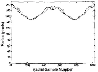
The radius function of a shape boundary that is aligned along its axis of s y e t r y can he used to compare and quantify the actual shape. If the shape were a perfect circle, the radius function would have a constant value, equal to the radius of the circle. If the shape were perfectly symmetrical, then the radius function would be an even function, and its Fourier transform would contain only cosine components. A shape that is asymmetrical will have a Fourier transform with both sine and cosine components, and this is the general case. By taking the Fourier transform of the radius function, we can derive a description of its shape using harmonic coefficients.

Figure 7 shows the sine and cosine transform coefficients of the radius function shown in Figure 6, for up to 50 harmonics.

5 Measuring

Asymmetry

If the shape boundary were perfectly symmetrical, then its radius function would be the same if it were reversed-that is, if the shape boundary were Aipped about its axis of symmetry. A simple measure of asym-

metry is, therefore, the sum of squared differences between the radius function and its reflection. However, such a measure would depend on the overall size of the skull. To obtain a normalised value of asymmetry, the

sum of squares is divided by the square of the average radius. For set of radial samples R = { r l , .

. .

,

~ ~ 0 2 ~ ) . the asymmetry is measured as:

We call this the degree of asymmetry of a shape boundary. The shape boundary in Figure 4 has a degree of asymmetry of 0.3288. This degree of asymmetry will later be used for shape classification.

.o

20

43 Ga L i & &E

Radial Sample Number

Fib- 6 102bmmple Rodivs Function Thhc radius function o f lhc

rhapc bovndary shown in Fib- 4. Ifs rdlcction Is overlaidon thc plot.

J

4

( 0 x1 10 a0 I O (a

Harmonic Number

Fiyre 7 : Harmonic Conmnl nfNorndrredShappe E o u n d q The spec- mrm of Be normalised rhapc froom Fib- 4 , up to 50 soctlkimts.

The harmonic serjes of sine and cosine components ex- tends from zero (a basic circle) up to harmonic number 512. This full series is an equivalent representation of the radius function, since each may be derived from the other. However, if the harmonic series is truncated at a low harmonic number, then we have an approximate representation of the shape boundary. For example, with no harmonics, the approximate shape is a circle.

By taking the s u m of squared differences between the actual and approximated radius function, we can estimate a percentage error. This is shown

in

Figure 8 for up to

(5)

harmonics (five sine and five cosine). It has previously been noted that 21 coefficients can be sufficient for some biological characterisation and that spectral power drops

rapidlyaflersevencoefficients[6]. Ithasalsobeenshown that a small number of coefficients can be adequate for image matching purposes

[SI.

Figure 7 supports these notions for typical brain shape.

Harmonic mnlenl

F i y r c 8 Sum of squared diff-ccr bchv- lhe a c t d and modelled

radius h c l i o n , for up to 50 harmonicr.

If we use only cosine harmonics, then the approxim- tion has perfect bilateral symmetry The high-frequency harmonics contribute the 'roughness' of the shape bound- ary while most of the overall shape is described by low- frequency harmonics. Figure 9 demonstrates the wntri- butions of sine and cosine harmonics.

-

6.1 Curvature

Landmarks

Our Fourier analysis provides a superposition of pure cosine waves that describe shape boundaries. The use

of law-frequency harmonics results in a 'smooth' shape boundary and provides robustness in the presence of noise. Therefore, it i s simple to fmd local "a and minima (extrema) of curvature. It,is typical that a bmin shape boundary will contain several curvature extrema and that these mathematical quantities will correspond to areas such as the frontal poles, occipital poles, and the lateral edges of the brain. It is possible to quantitatively measure the position and magnitude of the curvature ex- trema for classification purposes.

6.2 Problem Scenarios

The interpretation of u l i s shape analysis is only well de-

fined for the bulk of nil focal cases

(as

diagnosed by L.C.)

171

with no great dissimilarities between the brain hemispheres. Although OUT unsupervised algorithm can ob-

tain numerical results for other cases, the results may not be interpretable in the same way. In future, detec- tion of these situations may lead to intelligent analysis of unusual feature or abnormalities.

For example, heads such as the one shown in Fig- 10 are physiologically asymmetric to a large degree. No- tice that the cosine harmonics have captured the principal symmetric shape features such as the broad frontal area, the low lateral convexity, and the roundness in the posterior regjon.

The quantification of shape is simplified if the shape boundaries of a person's hemispheres have equal perime-

ter and radial occupancy. Figure 11 illustrates a situation where neither of these is true. Currently, the interpretation of our c m n t algorithms in

this

situation is unde- fined.

(6)

F i y r c 11: Uncenoin Inrcrpreioiion Thc paticnt's ~ O Y points to the

Lap of thc h n q s in Lhis orknwion. Notics thc x ~ v c p i t i o n s of

the h-rphercr and ~ ( I y c m . ~ such BS thc intcrhcmisphcric (central) fissure a d f m d h- of L c latemi v&clcr.

7 Classification

of

Shape

We can classify shapes using harmonic coefficients, curvature [3], asymmetry, and error between the complete and low-frequency harmonic content.

The harmonic coefficients were found to be statisti- cally Gaussian and, as predicted by Christopher (1974) [SI, independent. As such, no correlation or 'clustering' was seen. However, superposition of harmonics leads ta

various typical shapes, shown in Figure 12.

In

general, the second harmonic is significant in heads that are much longer than they are wide. The thud harmonic is significant in heads that have a broad posterior combined with a narrower anterior. The fourth and fifth harmonics capture convexity at the front and both sides.

It was found that degrees of asymmehy above 2.3 corresponded to patients with focal bone abnormalities, including foreign objects. It was also found to be indica- tive of mis-selected images (the bi-parietal slices were selected automatically by an unsupervised algorithm). ASymmeiries above 1.0 corresponded with large visible imbalances (including differences in length) between the hemispheres. Asymmetries between 0 and 1.0 corresponded with typical shapes. The majority of cases fell into this latter category. No shape boundaries were

found

to have zero asymmetry. T h e mean was OS4 and standard deviation was 0.5 for 528 cases.

It was found that the shape boundaries could be represented to within 3% by the use of only five cosine har- monics. Thus, each shape boundaq can be quantified to this accuracy with only six parameters: the harmonics Plus a size factor. By adding more harmonics, the shape houndanes can be quantified more accurately with little increase in the number of parameters. However, it was found that r e l a h g the magnitudes of the low-frequency harmonic coefficients alone did not enable automated dis- crimination of shape boundary appearance. Some past research has suggested that symmetry-axis lateral sampling 191 or eigenshape approaches [IO] could be of value.

It was found that the curvawre extrema can describe shape boundaries according to increasing outward curva-

ture ('cups') or decreasing curvature, as well as describ- ing big and small end discs as in Blum (1973) [ I l l . By calculating a chain ofcurvature features

[IZ],

the human- perceived shape can be classified and compared between cases. Regions of boundary shape with high or low infor- mational content [13] can be descrhed in

this

way. For the cases examined, exactly four chain segments were present except in nine cases that had six, eight, or nine points. It appeared that these e x m points represented ar- cas oflow curvature with some cosine-wave artefacts.

(7)

Description

I

Identified

I

Frontal: broad I 180

I

Number of

Caws

~~ ~~~~ ~

Lateral Anterior: low convexity Lateral: excessive convexity Occipital: broad

9 Acknowledgements

This work was funded by the WA State Government Cen- tres of Excellence Progmn-ARCME.

258 57

115

References

[I] A. O ~ M U S , C. J. Yong-Hing, K A. Tong, and G. E. S&y, ‘A reliable method for measurement and nor- malization of pediatric hippocampal volumes,” Pe-

diatric Research, vol. 50, no. l, pp. 124-132,2001.

[21 I. Emelyanovq K. Parka,

L.

&la, R. Linggard, Y. Attikiouzel, K. Micbalak, N. Hicks,

P.

Rob- bins, and

E

Mastaglia, “Automatic Measurement of Brain Height from

CT

Scans,” lysEas F eWorld Scientific and Engineering Academy and Society)

Transactions on Circuits, vol. 1, no. 1, pp. 165-168, 2002.

[3] W.-Y. Ma and B. S. Manjunath, “Netra: A twlbox for navigating large image databases:’ Multimedia Systems, vol. 7,no. 3, pp. 184-19X. 1999. [4] R. L. Anstey and D. Delmet, “Fourier analysis of

zooecial shapes io fossil tubular bryozoans,’’ Geo-

logical Society of America Bulletin, vol. 84, no. 5, pp. 1753-1764, 1973.

151

Y.

Rui, A. She, and T. Huang, ‘‘Modified fourier de-

scriptors for shape representation

-

a practical ap-

proach:’ in First International Workhop on Image Databases andMulti Media Search, 1996. [6] R. Tello, “Fourier descriptors for computer graph-

ics:’ IEEE Transactions on System, Man. and Cy-

berneticr, vol. 25, pp. 861-865, May 1995.

[7l

L. A. Cala, G. W. Thickbroom, I. L. Black, D. W. K. Collins, and F. L. Mastaglia, “Brain density and cerebro-spinal fluid space size:

Cr

ofnormal volun- teers:’ American Journal o f N ~ r a d i o l o g y , vol. 2, pp.4147, Jan-Feb 1981.

[SI R. A. Christopher and

J.

A. Waters, “Fourier series as a quantitative descriptor;’ Journal of Paleontol-

00, vol. 48, pp. 697-709.1974.

[9] H. Blum and R. Nagel, “Shape description using weighted symmetric axis features,” Pattern Rccog- nition, vol. 10, no. 3,pp. 167-180, 1978.

vol. 25, pp. 107-138, 1999.

[IO] N. McLeod, “Eigenshipe analysis:’ Paleobiology,

[I11 H. Blum, “‘Biological shape and visual sciFce (part I):’ Journal of Theoretical Biology, vol. 38, pp. 205-287, 1973.

[I21 F. Leymarie and iyi. D. Levine, “Curvature morphol- ogy,” Tech. Rep. TR-CM-88-26, Cenke for Intelli- gent Machines, McGill University, 19x8.

1131 M. Leyton, “Symmetry-curvature duality:’ Com- puter Ksion Graphics and Image Processing,

vol. 38, pp. 327-341, 1987.