The Thirty-Third AAAI Conference on Artificial Intelligence (AAAI-19)
Model-Based Diagnosis for Cyber-Physical Production Systems
Based on Machine Learning and Residual-Based Diagnosis Models
Andreas Bunte
OWL University of Applied Sciences Institute Industrial IT
Langenbruch 6, 32657 Lemgo, Germany [email protected]
Benno Stein
Bauhaus-Universit¨at Weimar Faculty of Media, Webis Group99421 Weimar, Germany [email protected]
Oliver Niggemann
OWL University of Applied SciencesInstitute Industrial IT
Langenbruch 6, 32657 Lemgo, Germany [email protected]
Abstract
This paper introduces a novel approach to Model-Based Di-agnosis (MBD) for hybrid technical systems. Unlike exist-ing approaches which normally rely on qualitative diagno-sis models expressed in logic, our approach applies a learned quantitative model that is used to derive residuals. Based on these residuals a diagnosis model is generated and used for a root cause identification. The new solution has several advan-tages such as the easy integration of new machine learning algorithms into MBD, a seamless integration of qualitative models, and a significant speed-up of the diagnosis runtime. The paper at hand formally defines the new approach, out-lines its advantages and drawbacks, and presents an evalua-tion with real-world use cases.
Introduction
Current trends in production lead toward intelligent modular production systems, called Cyber Physical Production Sys-tem (CPPSs). Modular CPPSs are highly adaptive and can be configured in many different ways to produce a broad range of products. If such a CPPS fails, operators may not have gathered sufficient experience with the current configu-ration, and efficient manual diagnoses becomes harder if not impossible. An adaptive diagnosis system is considered the silver bullet to tackle a quick and reliable CPPS repair.
However, diagnosis concepts from today’s production systems are not applicable in this regard: Heuristic meth-ods, such as alarm generation, are hard to create and main-tain for large, quickly changing CPPSs and require too much manual engineering effort. Model-based approaches can be used for discrete CPPSs, but the models have to be both cre-ated and tested manually after every system adaption. Ad-ditionally, the diagnosis runtime become an important issue in large systems (Stern et al. 2015). Nevertheless, the MBD approach is promising for the future needs.
Model-Based Diagnosis (MBD) was introduced by Re-iter (1987) as Diagnosis from First Principles and by de Kleer and Williams (1987) as General Diagnostic Engine (GDE). It is a generic diagnosis technique which uses a sys-tem model in logic as a basis. Observations from the syssys-tem are added and they are expected to stay consistent with the
Copyright c2019, Association for the Advancement of Artificial Intelligence (www.aaai.org). All rights reserved.
system model if all components function correctly. If an in-consistency between the system model and an observation is detected, assumptions about the correct behavior of compo-nents are withdrawn until all inconsistencies disappear; the withdrawn assumptions are hence called diagnoses. This ap-proach also has limitations, especially when MBD is used for large, dynamic, and especially, hybrid CPPSs.
Challenge 1:Integration of Continuous Models.
MBD requires a system description in a suitable logic (Re-iter 1987) which makes MBD predestined for discrete sys-tems. But CPPSs are typically hybrid and combine both value discrete and value continuous variables. Therefore, models of multiple continuous variables have to be inte-grated into the diagnosis system: often, a change in the val-ues of discrete variables leads to a different system behavior, called a mode change (Niggemann and Lohweg 2015). Due to a mode change, the system’s models are changed and con-tinuous signals can shift abruptly. For example, turning on a heater triggers a mode change and will increase the power consumption by entering a new mode.
Challenge 2:Creation of Diagnosis Models.
The creation of a holistic qualitative model, which is re-quired for existing approaches, has to cover the whole sys-tem description. Especially in large CPPSs it is challenging to create such models since they are often designed manu-ally. It requires a lot of knowledge about the system and its causalities, and only experts can create them. However, even for experts it is time consuming and costly. Since CPPSs are adaptive, the models may need to be adapted often, which is not feasible. Hence, for CPPSs the models should be learned automatically (Niggemann and Lohweg 2015).
Challenge 3:Diagnosis Runtime.
The diagnosis runtime is challenging for large-scale sys-tems (Stern et al. 2015). The computation of the often used minimal cardinality diagnosis, a diagnosis with the smallest number of components, isNP-hard. I.e., algorithms have an exponential runtime with respect to the number of compo-nents (Metodi et al. 2014). To enable an efficient diagnosis for large-scale CPPSs, the search space has to be reduced.
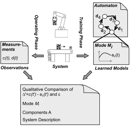
This model is comprised of two submodels:(i)an automa-ton which models the mode changes triggered by discrete variablesdiand(ii)a model describing the behavior of con-tinuous variablesec(t)for each modeMi. Note that several approaches exist to learn such models, see “Related Work“.
Second, in the operating phase, observations of contin-uous variables c(t) and discrete variables d(t) (top, left-hand side) are made in the running system. For each point in timet, a static diagnosis model (bottom of the figure) is generated, which comprises a system description, the health state of the system’s components and observations. The ob-servations contain the current residuals, the current mode, and the truth values of the discrete variables.
System
Mode Mi Automaton
d1 d3 d4
d2
Diagnosis Model for Point in Time t' Qualitative Comparison of
∆'=c(t') - ec(t') and ε
Mode Mi
Components A System Description
T
raining Phase
Operating Phase
Measure-ments
c(t), d(t)
Observations
ec(t)
LearnedModels
Figure 1: The main idea of the new RDA.
The contribution of this paper is an online diagnosis ap-proach for dynamic hybrid and non-linear CPPSs that sig-nificantly extends the current state of MBD:(i) RDA pro-vides a generic diagnosis approach for CPPSs that uses quantitative models which can be represented by multiple formalisms (challenge 1);(ii) learned models can be used for the diagnosis which reduce the modeling effort signifi-cantly (challenge 2);(iii)the CPPS is separated into modes which can be automatically learned by a finite automaton (challenge 1 + 2);(iv)RDA applies a residual-based diagno-sis which reduces the diagnodiagno-sis runtime, but still enables the usage of traditional MBD algorithms, so that existing high-performance algorithms can be used (challenge 3).
The paper is structured as follows: First, we will present the approach and provide an example. We then give a brief overview of related work. This is followed by an empirical evaluation which proves whether the challenges are properly addressed or not. Finally, we conclude the work and give a short overview about future topics.
Proposed Approach
In the following, RDA is presented. At first, definitions are introduced which are needed for the proposed hybrid diag-nosis (challenge 1). Then a small example is used to clarify how the approach works, therein we focus on the continuous part. Finally, the algorithm is introduced which consists of a training phase (challenge 2) and an operating phase, where the latter does the optimization (challenge 3).
Integrating Continuous Models
We use the following definitions in this work, to enable an integration of continuous models into MBD.
Definition 1 Ahybrid CPPSis defined as a set of devices A = {ai | i ≤ n;i, n ∈ N}. Eachai ∈ Ahas properties which are represented by a set of variablesV ={vj |j ≤ m;j, m∈N}, withV =C∪D, C∩D=∅. WhereasCis a set of value continuous variables andD is a set of value discrete variables.
Please note that the defined CPPS consists of a set of de-vices, which means that it is an automated system which always acts similar in a non-faulty case. That means there should be no human in the loop, because of the thereby in-jected randomness.
Definition 2 A variable v ∈ V is observable if its value can be determined at each point in time during the systems’ runtime.
There are mainly two reasons why a variable might not be observable:(i)it is technically not possible to determine the value, e.g. the distribution of chemicals in a reactor or (ii) because no proper sensor is installed, e.g. to reduce costs.
Definition 3 The continuous model of a hybrid CPPS A is defined as a set of functions R = {ec | c ∈ C, ec : R+ → R,}. Each function ec returns the expected value for an observable continuous variablec ∈ Cat a point in timet∈R+.
There are many formalisms that can be used for the repre-sentation of continuous variables. Some of them enable the continuous models to be learned, as we will show later on.
The continuous model enables a quantitative residual ∆
for every continuous variable to be determined, which is the difference between the measured value of a variable and its expected value.∆c=c(t)−ec(t)at a specific timet∈R+ for a continuous variablec∈C, whereec(t)is the expected value ofcat timet.
Definition 4 A qualitative residual for each continuous variablec ∈ C at each point in timet ∈ R+ can be de-fined by the following predicates:
• s0(c)iff|∆c| ≤ε
• s−(c)iff|∆c|> εand∆c<0
• s+(c)iff|∆
c|> εand∆c>0
ε∈R+is a threshold for the residual that is acceptable to assign the non-faulty qualitative residuals0to a variablec.
The ok-assumption is also referred to as thehealth state of a component.
Definition 6 A hybrid system description SDH describes
the systems’ causalities of hybrid systems and consists of a set of first order logic (FOL) sentences, including the pred-icates ok-assumption and qualitative residuals, but does not include quantifiers.
The qualitative residualss−ands+are typically modeled with a negation in the hybrid system description, since their occurrence is not expected during normal operation.
Definition 7 The componentsCOMPS is a set of all de-vicesCOMPS =A.
Definition 8 Theobservations OBS is a finite set of FOL sentences that represent observations about the system.
That means, the observations represent discrete variables and the qualitative residuals of observable continuous vari-ables. Since we also allow non-equidistant discrete time steps, theOBS can be updated at every point in timet ∈
R+.
The presented approach can be used for some systems, but it is challenging to model complex shapes of the continuous variables, because shapes mainly dependent on the systems’ mode. Therefore, we divide the system into different modes. Thus, the continuous variables have to be modeled for every mode, but the modeling per mode is much easier.
Definition 9 Afinite automatonfor a hybrid CPPS is a 3-tupleE= (M,Σ, T), where:
• M is a finite set of modes. Each modem∈M is a tuple m= (id,u), whereidis a unique identifier for the mode and u is a vector that represents the truth values of all discrete variablesu= (d0, ..., dn)T, d0, ...dn∈D.
• Σis the alphabet, the set of events, where an event is a change of the truth value of at least one discrete variable.
• T ⊆ M ×Σ×M gives the set of transitions, e.g. for a transitionhm, b, m0i,m, m0 ∈ M are the source and destination mode, andb∈Σis the trigger event. (Maier 2014)
We use the unique identifiers of the modes as variable names in FOL to describe whether the CPPS is currently located in a certain mode or not. For example, if its vari-ableM1holds true, the CPPS is in modem1 = (M1,u).
The mode identifierM1that represents the modem1is in-tegrated as FOL variable M1 to a sentence in the hybrid system descriptionSDH if the FOL sentence holds true in
modem1. The observationsOBS contain the mode identi-fier of the mode that holds true, at the current point in time. However, the system must not change its mode during a di-agnosis session. Additionally, the whole system should be synchronous to determine modes properly. An asynchronous part of the system would cause much more modes and thus much more training data to create a suitable model. Anyway, the modes provide a context and this enables the detection of not only point anomalies but also contextual anomalies, because a specific behavior is only suitable in a certain con-text.
Definition 10 Theclock is a continuous variablet ∈ R+ that increases linear strictly monotonically and is set to zero by changing the modem∈M of the finite automatonE. In modeless systems, clock and time are the same.
The structure of the RDA in the operational phase is shown in Fig. 2, where white boxes are components that do not differ from traditional MBD, whereas grey boxes are adapted for RDA. Arrows represent the flow of data. RDA processes the observations from the CPPS and the generic diagnosis model, which consists of an automaton, a contin-uous diagnosis model, the components, and a hybrid sys-tem description, to get a static diagnosis model. The static diagnosis model, which is used as input for the traditional MBD, consists of SDm,COMPSm, and OBS. The
sub-scripted m inCOMPSm andSDm indicates that it holds
true just for a single mode, so SDH = Sm∈MSDm and
COMPS =S
m∈MCOMPSm. We introduce the same
no-tation for the continuous modelR=S
m∈MRm.
Generic Diagnosis Model
CPPS Hybrid System Description SDH
COMPSm OBS
Continuous Model R Create Static Model
Traditional MBD-Algorithm
SDm Automaton E
Components COMPS
Static Diagnosis Model
Figure 2: Structure of the RDA during operational phase.
Example
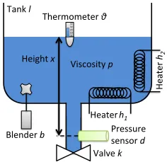
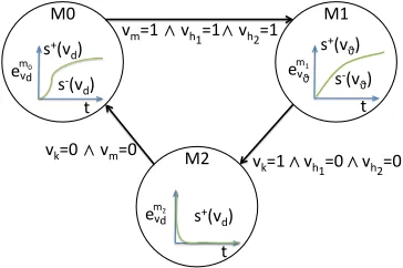
The approach is presented on a simple CPPS, shown in Fig. 3. It is a tank, where a defined volume of liquid is filled in (mode M0), a blender stirs the liquid during the heating process (mode M1) and then it is drained through a valve (mode M2). All shown components are part of the hybrid CPPS, sol, ϑ, b, h1, h2, d, k ∈A. To simplify the example,
we suggest the height of the liquid xand the viscosity of the productpas variables (properties) of tankl. The system contains the following variables vk, vb, vh1, vh2 ∈ D and
vx, vp, vϑ, vd∈C, where onlyvxandvpare not observable.
40 30 20 10 0
Thermometer θ
Heaterh1
He
ate
r
h2
Blender b Pressure sensor d
Height x
Valve k Viscosity p Tank l
Figure 3: Example of simple CPPS.
mode. Only one continuous variable is represented, because it is suggested the other variables constant to simplify the ex-ample. We define for modem1, whereemcϑ1(t)was identified
empirically:
ok(b)∧ok(h1)∧ok(h2)∧M1→s0(vϑ) ok(b)∧M1→ ¬s+(v
ϑ) ok(h1)∧ok(h2)∧M1→ ¬s−(vϑ)
SDm1
em1
cϑ (t) = 60−30·2
2.56e−4·t oR m1.
The mode includes the allocation of discrete variables to be true, e.g. forM1:vb∧vh1∧vh2∧ ¬vkis true. So, modes
are explicitly modeled by the automaton and thus represents the discrete values in the system descriptionSDH. Since we
can learn automaton, as we show later on,SDH only
con-tain relations between health state of components, modes and qualitative residuals, which simplify its creation signif-icantly. However, the whole system description just repre-sents the normal behavior, including situations that do not occur during normal operation. The qualitative residualss− ands+ have a negation to indicate that the behavior is not expected. Please note that these are not strong fault mod-els. Strong fault models also represent faulty behavior and enable a consistency, even if a component fails.
M0 M1
vm=1 ∧ vh1=1∧ vh2=1
vk=0 ∧ vm=0
evd s-(v
ϑ)
evϑ
m0 m1
s+(v d)
s-(v d)
M2
s+(v d)
emvd 2
s+(v ϑ)
vk=1∧v
h1=0∧vh2=0
t t
t
Figure 4: Automaton for the simple CPPS from Fig. 3.
In this example, we observeOBS ={s+(v
ϑ), M1, vb∧ vh1 ∧vh2 ∧ ¬vk}, since ∆cϑ > ε. This is not consistent
with the system description, it contradictsok(b)∧M1 →
¬s+(v
ϑ) if we assume all components are working cor-rectly. The consistency is achieved by canceling the ok-assumption forb, which is the only, as well as the correct, diagnosis.
Creating Diagnosis Models
The general (non-static) diagnosis model contains a hybrid system descriptionSDH, the componentsCOMPS, an
au-tomatonE and a continuous modelR. TheSDH only
con-tains relations between health state of components, modes, and qualitative residuals. So, the creation ofSDH is much
easier, since neither the modes nor the continuous variables have to be modeled. Before we introduce the algorithm for the training phase, we introduce some more notations.Vt refers to the measured values of variables V at specific
timet ∈ R+.V∗ is a set of measured values of the vari-ablesV at different points in timeV∗ =S
t∈[t1,t2]V
twith
t1, t2 ∈ R+, called historical data. AsV = C ∪D holds true, both notations can be used equivalently:Vt=Ct∪Dt andV∗ =C∗∪D∗. Additionally, all symbols from defini-tions 1 – 10 are the same as in the algorithms.
The training phase is presented in Algorithm 1. In line 1, a finite automaton is learned by using discrete variable names and historical data. The historical data have to represent the normal behavior of the CPPS without any faults. Not all vari-ables have to be used to learn the model. There might be some variables which should not be used, such as variables controlled by pulse duration modulation, since they toggle for a long time without changing the mode in the sense of the process. Mostly there is a flag that can be used instead. All modes of the learned automaton are determined (line 2) and used to iterate over each modes (line 3) to learn the continu-ous model for each mode. Therefore, the continucontinu-ous model Rmfor mode m is initialized by an empty set (line 4). Then, the expected valuesem
c for all continuous variablescin the mode m are learned, based on historical data, and added to Rm(line 6 + 7). Finally, the continuous model of the mode Rmis added to the overall continuous modelR(line 8) and the automaton and the overall continuous model are returned (line 9).
Algorithm 1:Learning Modes and Continuous Model Input:variablesV =C∪D, historical data
V∗=C∗∪D∗
Output:finite automataE, continuous modelR
1 E←learnAutomaton(D, D∗) 2 ModesM ←getAllM odes(E) 3 forallmodesm∈M do
4 Rm← ∅
5 forallcontinuous variablesc∈Cdo
6 emc ←learnExpectedV alues(m, c, C∗)
7 Rm←Rm∪ {emc }
8 R←R∪Rm
9 returnE, R
Learning Modes: Some learning algorithms for finite au-tomata can be found in the literature, such as MDI (Car-rasco and Oncina 1994), ALERGIA (Thollard, Dupont, and de la Higuera 2000), RTI+ (Verwer 2010), BUTLA (Maier 2015), or OTALA (Maier 2014). All these algorithms learn automata without expert knowledge.
By reviewing the possible algorithms, we identified the Online Timed Automaton Learning Algorithm (OTALA) as a good choice. OTALA is an online learning algorithm that uses the current values of discrete variables to define modes, so there arek|D|possible modes, where|D|is the number
Learning Continuous Models:RDA is a generic approach, which does not limit the learning of continuous variables to a specific technique. Learning methods have to be compati-ble to definition 3, so that they provide an expected value at every point in time and thus enable RDA to determine quali-tative residuals regarding definition 4. Many methods known in machine learning fulfill these requirements.
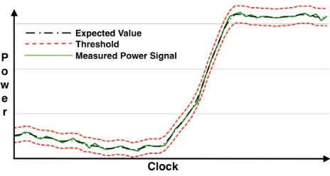
Figure 5: Measurement of the variable power with the ex-pected value, learned with regression, and boundaries.
As an example, we use non-linear regression to represent the power consumption during the operation mode of turning on a heater, which is performed after a short reaction time. In Fig. 5, the regression model (which determinesec(t)) and the threshold (ε) are shown as well as a measured signal. The model is learned with a two layer neural net with 48 neurons on the hidden layer, using the gradient descent al-gorithm with a learning rate of 0.001. As one can see, with this model it is possible to determine a residual∆for every point in time. So regression is one suitable method for the representation of continuous variables in RDA.
Diagnosis Runtime
The RDA algorithm is executed during the operational phase at a specific point in time t. At this point in time a static di-agnosis model is created by capturing the observations and the generic diagnosis model. Additionally, it is used to re-duce the search space and thus decrease the diagnosis run-time (challenge 3). This is achieved by computingSDmand
COMPSm. Therefore, all statements fromSDH are checked
if they hold true in the current mode, and only those state-ments are added to SDm. If they do not hold true, they
are not able to cause an inconsistency during diagnosis, so they need not be considered. All statements that are added toSDm are checked whether or not they contain a device
a∈COMPS, which reduces the search space and is mainly
responsible for the increased performance. Again, only those devices that appear in theSDm can cause an inconsistency.
All other devices do not need to be considered without loss of generality.
This computation is shown in the first part of algorithm 2. At first, the current mode is determined (line 1). Then the outputs are initialized with empty sets (line 2-4). All sen-tences of the hybrid system description are browsed through (line 5) and they are checked if they hold true in the
cur-rent mode (line 6). If the sentence holds true, it is added to the system description for the current modeSDm (line 7).
Furthermore, all components of the sentence are extracted and added toCOMPSm(line 8+9). This reduces the search
space for the diagnosis algorithm.
Algorithm 2:RDA Compute Diagnoses Input:variablesV, continuous variablesC,
measurementVt, finite automatonE, continuous modelR, hybrid system descriptionSDH, componentsCOMPS
Output:DiagnosesΩ
1 Modem←determineM ode(E, Vt)
2 SDm ← ∅
3 COMPSm ← ∅
4 OBS ← ∅
// Compute SDm and COMPSm
5 forallα∈SDH do
6 ifαholds true inmthen
7 SDm ←SDm∪α
8 ifαcontainsa∈COMPS then
9 COMPSm ←COMPSm∪a
// Compute OBS 10 forallv∈V do
11 ifv∈Cthen
12 ∆v←v(t)−ev(t)
13 OBS ←OBS∪determineResidual(∆v, ε)
14 else
15 ifv(t)then
16 OBS ←OBS∪v(t)
17 else
18 OBS ←OBS∪ ¬v(t)
19 OBS ←OBS∪getID(m)
20 Ω←computeDiagnoses(SDm,COMPSm,OBS)
21 returnΩ
The preprocessing of observations is necessary to perform the hybrid diagnosis with traditional MBD algorithms. Two steps are needed: determine the residuals for each continu-ous variable and determine the current mode. Discrete vari-ables are added directly to theOBS, since they do not re-quire any preprocessing. Algorithm 2 shows how to compute
Related Work
Model-Based Diagnosis Although MBD has been well known for over 30 years, it is still an active field of re-search. One focus of research is to improve the algorithms’ performance, since the complexity is a major challenge in MBD (Feldman, Provan, and van Gemund 2010). There are a some fast algorithms available, such as SAFARI (Feldman, Provan, and van Gemund 2010), SDA (Siddiqi and Huang 2011) or SATdB (Metodi et al. 2012). Each of these algo-rithms optimizes the computation of diagnoses and performs better than the previous ones, often by at least one order-of-magnitude. Jannach, Schmitz, and Shchekotykhin (2015) introduce another algorithm-based approach by parallelize hitting set computation, which utilize a multi-core computer better than the usual algorithms and reduce the computation time by up to 85 %. Since we use traditional MBD algo-rithms, our approach is compatible with those works and they can be used for an efficient implementation.
But not only algorithms are used to improve the perfor-mance, Guo et al. (2011) merge components with same con-straints to the output set. This reduces the number of com-ponents and thus reduces the runtime of the diagnosis algo-rithm. The work at hand also reduces the number of compo-nents, but we use information about modes and do not search for similar constraints. The approach of Guo et at. is compat-ible, so it can be applied to every mode of the work in hand to increase the performance further. However, there is potential for a further increase in performance, e.g. Perdomo-Ortiz et al. (2017) applied MBD to a quantum computer.
Qualitative Reasoning The idea of qualitative reasoning (QR) is to reason like humans, since they do not calculate differential equations for inferences, but mostly use qualita-tive information. Many approaches can be found in the liter-ature, such as (Kuipers 1986), (Wiley, Sammut, and Bratko 2014) or (Izmirlioglu and Erdem 2018). The approach pre-sented in this paper does not use classical concepts of QR. The only concept we use from QR is discretization of residu-als ashigh/+,low/-oras expected/0. But we use a threshold to rate them and not a sign-function as is typical for QR.
Machine Learning Many approaches can be found in lit-erature, which focus on the learning of system models to de-tect anomalies, such as (von Birgelen and Niggemann 2017; Hranisavljevic, Niggemann, and Maier 2016). However, those approaches are not able to identify precise root causes. If they do, it is based on a similarity measurement between the expected and the observed values. This can be helpful in detecting a wrong sensor value, but those methods are not able to identify more complex root causes. For example, the chaining effect propagates over multiple modules before it is detected and thus they are complex to identify.
In the work at hand, machine learning is used to represent continuous variables over the time. Therefore, use nonlinear regression is used, which is realized by a neural net, regard-ing (Russell and Norvig 2010). But also other approaches can be used, such as deep neural networks and autoencoder (la Rosa, Yu, and Li 2016) or switched kalman filter (Nguyen and Goulet 2017). More details can be found in (Osborne et al. 2012) and (Gao, Cecati, and Ding 2015).
Hybrid Model Based Diagnosis There is a lot of work available that deals with the diagnosis of hybrid systems. Hybrid systems are mostly modeled as a combination of an underlying discrete model, where each state (we call it mode in this work) contains the representation of the con-tinuous signals, such as (Biswas et al. 2003; Grastien 2014; Taktak, Triki, and Kamoun 2017; Prakash, Samantaray, and Bhattacharyya 2017). We follow this paradigm in our work.
An often used modeling formalism for those systems are temporal causal graph (TCG) or hybrid bond graphs (HBGs) which can be transformed to a TCG for the further process-ing. Biswas et al. (2003) use TCG to model the hybrid sys-tem. An observer is implemented as a combination of ex-tended Kalman filter and a hybrid automaton which is used to determine residuals. The diagnosis is done in three steps: qualitative roll-back, qualitative roll-forward, and quanti-tative parameter estimation. The approach is demonstrated on a fuel transfer system of an aircraft. An extension of the work is represented in Narasimhan and Biswas (2007), where HBG are used for the modeling. Since the scalability of centralized diagnosis approaches is bad, Prakash, Saman-taray, and Bhattacharyya (2017) extend the HBG approach to a distributed algorithm for sequentially occurring faults in hybrid dynamical systems. The advantage of the decen-tralized algorithm is less needed computing power. A super-visory diagnoser handles the situation if more than one al-gorithm detects a fault. But the presented approach requires slow dynamics. The presented approaches only detect para-metric faults and they require significant manual effort, be-cause the models have to be created by experts. So, these ap-proaches are suitable for process industries, where discrete faults do not play a major role and where the system does not change regularly. Instead our approach is suitable for the manufacturing industry, where processes change regularly and discrete faults play a major role, e.g. a workpiece holder on a conveyor triggers a light barrier.
Voigt, Flad, and Struss (2015) introduce the application of MBD in a bottling plant by extending a traditional MBD al-gorithm. The authors represent the system with precise equa-tions and transform them into a qualitative mathematical de-scription. They used a real world application, but they use classical QR concepts for abstraction, not residuals, they are limited to total fault, i.e. system breakdown, and their envi-ronment does not change, so they create models manually.
Grastien (2014) introduces an approach for diagnosing hybrid systems with satisfiability modulo theories (SMT). He separates the system into states (modes), but he does not differentiate between continuous and discrete variables, they are all used to define states. The major drawback of his ap-proach is the diagnosis runtime.
Evaluation
This section consists of two parts: Evaluation of hybrid diag-nosis (challenge 1) and of the diagdiag-nosis runtime (challenge 3). The learning of models (challenge 2) is not evaluated on its own, it is covered in the evaluation of hybrid diagnosis, since wrong models will lead to a wrong diagnosis.
Evaluation of Hybrid Diagnosis
Two CPPSs are used to evaluate the diagnosis approach. To evaluate the approach on real-world CPPSs, we made the trade-off to use a small real-world system, instead of a large artificial one. The first is a demonstration plant of a modu-lar CPPS (called versatile production system (VPS)) in the SmartFactoryOWL that processes corn and makes popcorn from it. The CPPS consists of four modules, namely deliv-ery, storage, dosing, and production, which can be easily ad-justed regarding the current needs. In total the modules have 23 components, such as conveyor, level sensors, aspirator, heater or power meter. The components have three contin-uous variables (power meter, weight of corn, and weight of popcorn) and 20 binary variables (conveyor on/off, sensor on/off, etc.). A data set is used with a total of 34,973 ob-servations, where 27,187 present the correct behavior and have been used for learning. The observations were taken with equidistant time steps of 50 ms. We used eight differ-ent arrangemdiffer-ents with two to four modules. For example, if small batches are to be produced, the dosing module has to be used. Whereas this is not necessary if big batches are produced and the weight does not have to be so exact. In that case, the corn can be portioned by the runtime of the conveyor (VPS 6 in Fig. 6).
The OTALA algorithm was used to learn the automata which identified up to 13 modes for each arrangement. Then, the continuous models are learned within each mode. There-fore, we used non-linear regression, as described in the pre-vious section. We set the threshold, to decide whether a sig-nal is anomalous or not, manually.
As a second CPPS one of the well-known two-tank sys-tems (TTS) in two different arrangements was used, because only two are possible with two tanks. Within the CPPS two tanks, pumps, values, heating, and mixing units perform a batch process, similar to the example in the previous section (see figure 3).
For evaluation, we injected 10 discrete and 10 continu-ous faults into each arrangement of both systems within dif-ferent modes. The evaluation was successful if an inconsis-tency was detected and the diagnosis algorithm provided di-agnoses that contain the effected component. Therefore, in-consistencies have to be detected, which require a correct continuous model and a proper threshold to detect contin-uous faults, and a correct conclusion of the diagnosis algo-rithm.
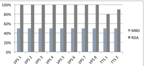
Fig. 6 shows a comparison between traditional MBD and RDA. Both approaches are able to identify all discrete faults, which were expandable since they use the same method for discrete faults. The MBD was not able to identify a con-tinuous fault in any system. In its extended version, RDA has identified all continuous faults in the VPS correctly and
0% 20% 40% 60% 80% 100%
VPS 1 VPS 2 VPS 3 VPS 4 VPS 5 VPS 6 VPS 7 VPS 8 TTS 1 TTS 2
MBD RDA
Figure 6: Comparison of MBD with RDA in CPPS.
85% of the continuous faults in the TTS. The not-detected faults are caused by undetected inconsistencies, because the residuals have been too small to reach the threshold. A lower threshold leads to more false positives, whereas a higher threshold leads to more false negatives. So, one has to make a trade-off between them, which might depend on the use case. In the examples above, we minimized the total faults. A decrease of the threshold led to an increase of the total number of faults, so it is use case specific that we did not get some faults positives. However, the root-cause for all de-tected faults was determined correctly. So, from a logical point of view, the diagnoses have been correct in all cases (challenge 1) and only the learned continuous models re-spectively the residuals have to be improved (challenge 2).
Evaluation of Diagnosis Runtime
To evaluate the diagnosis runtime, we used a MBD algo-rithm that we implemented on our own. There was no imple-mentation of a high-performance algorithm, as mentioned in ’Related Work’, available. To evaluate the diagnosis run-time we compared RDA with a traditional MBD approach, where both approaches use the same MBD algorithm. We only used discrete faults, so the hybrid diagnosis capabil-ity of RDA was not used. Since continuous faults are repre-sented as predicates, as discrete faults, there is no difference in the diagnosis runtime.
We used a generatedSDwith a different number of com-ponents. For two components the system description con-tains one mode and four statements. So the proportion was constant and set to a proportion similar to the model of the demonstrator in the previous section. For evaluation an iMac with 2,5 GHz Intel Core i5-2400S, 8 GB DDR3 RAM, and MacOS Version 10.13.1 was used.
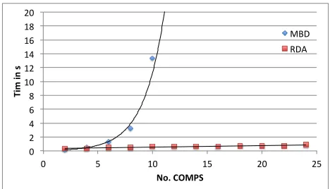
Fig. 7 presents the runtime in seconds to compute diag-noses over the number of components for the traditional MBD and for RDA. We computed one diagnosis in each mode and performed each computation 10 times to reduce side effects due to the non-real time operation system. The traditional MBD, marked by blue dots, shows an exponential correlation toCOMPS, whereas the optimized version with RDA, marked by red squares, shows a linear correlation to
COMPS, with a low rise. The linear correlation also holds
0 2 4 6 8 10 12 14 16 18 20
0 5 10 15 20 25
Ti
m i
n s
No. COMPS
MBD RDA
Figure 7: Runtime of RDA and a MBD. Due to representa-tion reasons, we did not print all experiments of the MBD.
in modeless systems (such as in the 2COMPS experiment, see Fig. 7) the traditional algorithm is slightly faster. This is because, RDA tries to optimize theSDandCOMPS, which is not possible in this case, but it still needs a short period of time. The optimization takes typically between 0,2% and 1% of the RDA runtime. We showed that RDA has a significant better performance (challenge 3) for large systems.
Conclusion
Three challenges have been identified and tackled in order to apply MBD to large hybrid CPPSs, namely, the integra-tion of continuous models, the creaintegra-tion of models, and the diagnosis runtime. The novelty of this paper is a diagno-sis algorithm RDA that learns quantitative models (train-ing phase), performs a diagnosis based on residuals, and, due to an optimized runtime, is able to create diagnoses for large hybrid CPPSs (operational phase). A finite automaton is learned that covers the discrete variables, and within each state a continuous model is learned. As a result, the manual modeling effort boils down to modeling only the relations between modes, qualitative residuals, and the health state of components. Our evaluation shows that the approach is able to identify discrete and continuous faults, and that it finds the correct diagnosis in most cases. Due to its runtime op-timization the approach can be used for large CPPSs; the larger the CPPS, the bigger is the advantage of RDA, com-pared to traditional MBD. The approach is limited with re-gard to complex continuous behaviors within a single mode, such as CPPS with only continuous or only rarely switching discrete variables, as shown with the two-tanks system.
One major issue for further work is the integration of re-action times and thus the aggregation of modes. Because reaction times lead to multiple modes for the same action, e.g. if a tank is drained by opening a valve, it takes a short time before the maximum level sensor will switch its value, which indicates that the level has dropped. The change of the sensor leads to a mode change, but has no influence on the behavior and thus similar modes have to be modeled mul-tiple times. Handling these situations reduces the modeling effort additionally. Another issue is the improvement of con-tinuous models, since the non-detected faults in the
evalua-tion are based on an undetected deviaevalua-tion of the variables. The improvement can be achieved by an automatic selec-tion of an appropriate machine learning method along with an adaptive threshold that learns the expected deviation. Up until now, the threshold is set in a manual process that re-lies on expert knowledge and experience, since the threshold is effected by many parameters such as model quality and use case requirements. An adaptive threshold will also en-able the diagnosis with less training data, since a poor model can be used with an high threshold which decreases if more data are available for the model learning and thus the model quality increases. Another requirement of CPPSs is that they have to stay in their mode during diagnosis which might be hard to guarantee in real applications. Therefore, the algo-rithm could be extended to achieve a multimode diagnosis which is able to use the information from different modes. This has the advantage that the diagnoses would be smaller and thus more precise, since more observations are added.
Acknowledgments
The work was supported by the German Federal Min-istry of Education and Research (BMBF) under the project ”KOARCH” (funding code: 13FH007IA6).
References
Biswas, G.; Simon, G.; Mahadevan, N.; Narasimhan, S.; Ramirez, J.; and Karsai, G. 2003. A robust method for hy-brid diagnosis of complex systems. IFAC Proceedings Vol-umes36(5):1023 – 1028. 5th IFAC Symposium on Fault De-tection, Supervision and Safety of Technical Processes 2003, Washington DC, 9-11 June 1997.
Carrasco, R. C., and Oncina, J. 1994. Learning stochas-tic regular grammars by means of a state merging method. In GRAMMATICAL INFERENCE AND APPLICATIONS, 139–152. Springer-Verlag.
de Kleer, J., and Williams, B. C. 1987. Diagnosing multiple faults.Artificial Intelligence32(1):97–130.
Feldman, A.; Provan, G. M.; and van Gemund, A. J. C. 2010. Approximate model-based diagnosis using greedy stochas-tic search.J. Artif. Intell. Res.38:371–413.
Gao, Z.; Cecati, C.; and Ding, S. X. 2015. A survey of fault diagnosis and fault-tolerant techniques – part i: Fault diag-nosis with model-based and signal-based approaches. IEEE Transactions on Industrial Electronics62(6):3757–3767.
Grastien, A. 2014. Diagnosis of hybrid systems with SMT: opportunities and challenges. InECAI, volume 263 of Fron-tiers in Artificial Intelligence and Applications, 405–410. IOS Press.
Guo, T.; Li, Z.; Guo, R.; and Zhu, X. 2011. Large scale di-agnosis using associations between system outputs and com-ponents. InAAAI Conference on Artificial Intelligence.
Izmirlioglu, Y., and Erdem, E. 2018. Qualitative reasoning about cardinal directions using answer set programming. In AAAI Conference on Artificial Intelligence.
Jannach, D.; Schmitz, T.; and Shchekotykhin, K. 2015. Par-allelized hitting set computation for model-based diagnosis. InAAAI Conference on Artificial Intelligence.
Kuipers, B. 1986. Qualitative simulation. Artificial Intelli-gence29(3):289 – 338.
la Rosa, E. D.; Yu, W.; and Li, X. 2016. Nonlinear system modeling with deep neural networks and autoencoders algo-rithm. InIEEE International Conference on Systems, Man, and Cybernetics (SMC), 2157–2162.
Maier, A. 2014. Online passive learning of timed automata for cyber-physical production systems. In IEEE Interna-tional Conference on Industrial Informatics (INDIN). Porto Alegre, Brazil.
Maier, A. 2015. Identification of Timed Behavior Models for Diagnosis in Production Systems. Ph.D. Dissertation, University of Paderborn.
Metodi, A.; Stern, R.; Kalech, M.; and Codish, M. 2012. Compiling model-based diagnosis to boolean satisfaction. In AAAI Conference on Artificial Intelligence.
Metodi, A.; Stern, R.; Kalech, M.; and Codish, M. 2014. A novel sat-based approach to model based diagnosis.J. Artif. Int. Res.51(1):377–411.
Narasimhan, S., and Biswas, G. 2007. Model-based di-agnosis of hybrid systems. IEEE Transactions on systems, manufacturing and Cybernetics37:348–361.
Nguyen, L. H., and Goulet, J.-A. 2017. Anomaly detection with the switching kalman filter for structural health moni-toring. Structural Control and Health Monitoring25(4).
Niggemann, O., and Lohweg, V. 2015. On the Diagnosis of Cyber-Physical Production Systems - State-of-the-Art and Research Agenda. InAAAI Conference on Artificial Intelli-gence.
Osborne, M.; Garnett, R.; Swersky, K.; and de Freitas, N. 2012. Prediction and fault detection of environmental sig-nals with uncharacterised faults. InAAAI Conference on Ar-tificial Intelligence.
Perdomo-Ortiz, A.; Feldman, A.; Ozaeta, A.; Isakov, S. V.; Zhu, Z.; O’Gorman, B.; Katzgraber, H. G.; Diedrich, A.; Neven, H.; de Kleer, J.; Lackey, B.; and Biswas, R. 2017. On the readiness of quantum optimization machines for in-dustrial applications.ArXiv e-prints.
Prakash, O.; Samantaray, A. K.; and Bhattacharyya, R. 2017. Model-based diagnosis of multiple faults in hybrid dynamical systems with dynamically updated parameters. IEEE Transactions on Systems, Man, and Cybernetics: Sys-tems.
Provan, G. 2009. Model abstraction for diagnosing hybrid systems. InInternational Workshop on Principles of Diag-nosis (DX).
Reiter, R. 1987. A Theory of Diagnosis from First Princi-ples.Artificial Intelligence32(1):97–130.
Russell, S., and Norvig, P. 2010. Artificial Intelligence: A Modern Approach. Series in Artificial Intelligence. Upper Saddle River, NJ: Prentice Hall, third edition.
Siddiqi, S., and Huang, J. 2011. Sequential diagnosis by abstraction. J. Artif. Int. Res.41(2):329–365.
Stern, R.; Kalech, M.; Rogov, S.; and Feldman, A. 2015. How many diagnoses do we need? InAAAI Conference on Artificial Intelligence.
Taktak, M.; Triki, S.; and Kamoun, A. 2017. Real time algo-rithm based on time series data abstraction and hybrid bond graph model for diagnosis of switched system. Engineering Applications of Artificial Intelligence59:51 – 72.
Thollard, F.; Dupont, P.; and de la Higuera, C. 2000. Prob-abilistic DFA inference using Kullback-Leibler divergence and minimality. InInternational Conf. on Machine Learn-ing, 975–982. Morgan Kaufmann.
Verwer, S. 2010.Efficient Identification of Timed Automata: Theory and Practice. Ph.D. Dissertation, Delft University of Technology.
Voigt, T.; Flad, S.; and Struss, P. 2015. Model-based fault localization in bottling plants.Advanced Engineering Infor-matics29(1):101–114.