Character-Level Language Modeling with Deeper Self-Attention

(1)

The Thirty-Third AAAI Conference on Artificial Intelligence (AAAI-19)

Character-Level Language Modeling with Deeper Self-Attention

Rami Al-Rfou,

*

_{Dokook Choe,}

*

_{Noah Constant,}

*

_{Mandy Guo,}

*

_{Llion Jones}

*

Google AI

1600 Amphitheatre Parkway Mountain View, California 94043

{rmyeid, choed, nconstant, xyguo, llion}@google.com

Abstract

LSTMs and other RNN variants have shown strong perfor-mance on character-level language modeling. These models are typically trained using truncated backpropagation through time, and it is common to assume that their success stems from their ability to remember long-term contexts. In this paper, we show that a deep (64-layer) transformer model (Vaswani et al. 2017) with fixed context outperforms RNN variants by a large margin, achieving state of the art on two popular benchmarks: 1.13 bits per character ontext8and 1.06 onenwik8. To get good results at this depth, we show that it is important to add auxiliary losses, both at intermedi-ate network layers and intermediintermedi-ate sequence positions.

Introduction

Character-level modeling of natural language text is chal-lenging, for several reasons. First, the model must learn a large vocabulary of words “from scratch”. Second, natural text exhibits dependencies over long distances of hundreds or thousands of time steps. Third, character sequences are longer than word sequences and thus require significantly more steps of computation.

In recent years, strong character-level language models typically follow a common template (Mikolov et al. 2010; 2011; Sundermeyer, Schl¨uter, and Ney 2012). A recurrent neural net (RNN) is trained over mini-batches of text se-quences, using a relatively short sequence length (e.g. 200 tokens). To capture context longer than the batch sequence length, training batches are provided in sequential order, and the hidden states from the previous batch are passed for-ward to the current batch. This procedure is known as “trun-cated backpropagation through time” (TBTT), because the gradient computation doesn’t proceed further than a single batch (Werbos 1990). A range of methods have arisen for unbiasing and improving TBTT (Tallec and Ollivier 2017; Ke et al. 2017).

While this technique gets good results, it adds complex-ity to the training procedure, and recent work suggests that models trained in this manner don’t actually make “strong” use of long-term context. For example Khandelwal et al. (2018) find that a word-based LSTM language model

*_{Equal contribution.}

only effectively uses around 200 tokens of context (even if more is provided), and that word order only has an effect within approximately the last 50 tokens.

In this paper, we show that a non-recurrent model can achieve strong results on character-level language modeling. Specifically, we use a network of transformer self-attention layers (Vaswani et al. 2017) with causal (backward-looking) attention to process fixed-length inputs and predict upcom-ing characters. The model is trained on mini-batches of se-quences from random positions in the training corpus, with no information passed from one batch to the next.

Our primary finding is that the transformer architecture is well-suited to language modeling over long sequences and could replace RNNs in this domain. We speculate that the transformer’s success here is due to its ability to “quickly” propagate information over arbitrary distances; by compar-ison, RNNs need to learn to pass relevant information for-ward step by step.

We also find that some modifications to the basic trans-former architecture are beneficial in this domain. Most im-portantly, we add three auxiliary losses, requiring the model to predict upcoming characters (i) at intermediate sequence positions, (ii) from intermediate hidden representations, and (iii) at target positions multiple steps in the future. These losses speed up convergence, and make it possible to train deeper networks.

Character Transformer Model

Language models assign a probability distribution over to-ken sequencest0:Lby factoring out the joint probability as follows, whereLis the sequence length:

Pr(t0:L) =P(t0)

L

Y

i=1

Pr(ti|t0:i−1), (1)

To model the conditional probability Pr(ti|t0:i−1), we

train a transformer network to process the character se-quencet0:i−1. Transformer networks have recently showed

significant gains in tasks that require processing sequences accurately and efficiently.

(2)

t0 t1 t2 t3

t4

T

ransformer

La

y

ers

(a) Baseline

t0 t1 t2 t3

t1 t2 t3 t4

T

ransformer

La

y

ers

(b) Multiple Positions

t0 t1 t2 t3

t1 t2 t3 t4

T

ransformer

La

y

ers

(c) Layer Losses

t0 t1 t2 t3

t1

t2

t3

t4

t5

t1

t2

t3

t4

t5

T

ransformer

La

y

ers

(d) Multiple Targets

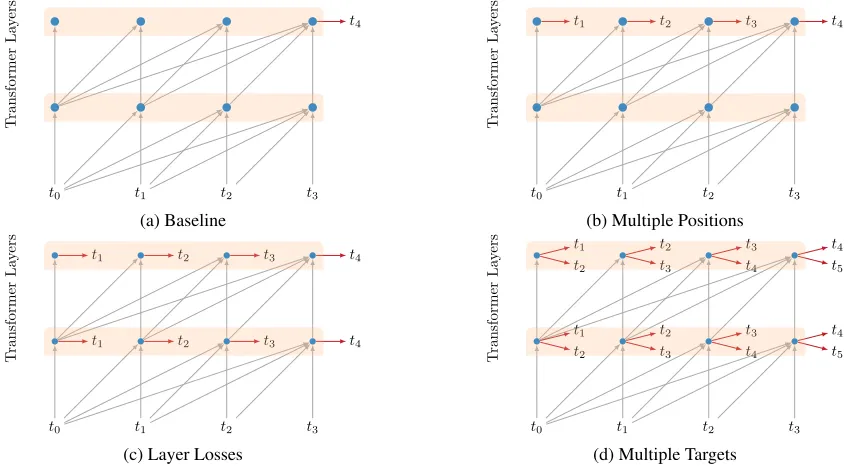
Figure 1: (a) A character transformer network of two layers processing a four character sequence to predictt4. The causal

attention mask limits information to left-to-right flow. Red arrows highlight the prediction task the network has to learn. (b) Adding intermediate position prediction tasks to our network. Now, we predict the final character t4 and all intermediate

characterst0:3. All of these losses contribute equally during training. (c) Adding prediction tasks for the intermediate layers.

For this example of two layers, the losses of the intermediate layer prediction tasks will be absent after finishing 25% of the training. (d) Adding two predictions per position.

two fully connected sub-layers. For more details on the transformer architecture, refer to Vaswani et al. (2017) and thetensor2tensorlibrary1.

To ensure that the model’s predictions are only condi-tioned on past characters, we mask our attention layers with a causal attention, so each position can only attend leftward. This is the same as the “masked attention” in the decoder component of the original transformer architecture used for sequence-to-sequence problems (Vaswani et al. 2017).

Figure 1a shows our initial model with the causal atten-tion mask limiting informaatten-tion flow from left to right. Each character prediction is conditioned only on the characters that appeared earlier.

Auxiliary Losses

Our network is, to our knowledge, deeper than any trans-former network discussed in previous work. In initial exper-iments, we found training a network deeper than ten layers to be challenging, with slow convergence and poor accuracy. We were able to deepen the network to better effect through the addition auxiliary losses, which sped up convergence of the training significantly.

We add several types of auxiliary losses, correspond-ing to intermediate positions, intermediate layers, and non-adjacent targets. We hypothesize that these losses not only speed up convergence but also serve as an additional regu-larizer. During training, the auxiliary losses get added to the

1

https://github.com/tensorflow/tensor2tensor

total loss of the network with discounted weights. Each type of auxiliary loss has its own schedule of decay. During eval-uation and inference time, only the prediction of the final position at the final layer is used.

One consequence of this approach is that a number of net-work parameters are only used during training—specifically, the parameters in the output classification layers associated with predictions made from intermediate layers and predic-tions over non-adjacent targets. Thus, when listing the num-ber of parameters in our models, we distinguish between “training parameters” and “inference parameters”.

Multiple Positions First, we add prediction tasks for each position in the final layer, extending our predictions from one per example to|L|(sequence length). Note, predicting over all sequence positions is standard practice in RNN-based approaches. However in our case, since no informa-tion is passed forward across batches, this is forcing the model to predict given smaller contexts—sometimes just one or two characters. It is not obvious whether these sec-ondary training tasks should help on the primary task of pre-dicting with full context. However, we find that adding this auxiliary loss speeds up training and gives better results (see Ablation Experiments below). Figure 1b illustrates the task of predicting across all sequence positions. We add these losses during training without decaying their weights.

(3)

we add predictions for all intermediate positions in the se-quence (see Figure 1c). Lower layers are weighted to con-tribute less and less to the loss as training progresses. If there arenlayers total, then thelth_{intermediate layer stops} con-tributing any loss after finishingl/2nof the training. This schedule drops all intermediate losses after half of the train-ing is done.

Multiple Targets At each position in the sequence, the model makes two (or more) predictions of future characters. For each new target we introduce a separate classifier. The losses of the extra targets get weighted by a multiplier of 0.5 before being added to their corresponding layer loss.

Positional Embeddings

In the basic transformer network described in Vaswani et al. (2017), a sinusoidal timing signal is added to the input sequence prior to the first transformer layer. However, as our network is deeper (64 layers), we hypothesize that the tim-ing information may get lost durtim-ing the propagation through the layers. To address this, we replace the timing signal with a learned per-layer positional embedding added to the in-put sequence before each transformer layer. Specifically, the model learns a unique 512-dimensional embedding vector for each of theLcontext positions within each ofNlayers, giving a total ofL×N×512additional parameters. We are able to safely use positional embeddings for our task, as we don’t require the model to generalize to longer contexts than those seen during training.

Experimental Setup

Datasets

For evaluation we focus mainly ontext8(Mahoney 2009). This dataset consists of English Wikipedia articles, with su-perfluous content removed (tables, links to foreign language versions, citations, footnotes, markup, punctuation). The re-maining text is processed to use a minimal character vocab-ulary of 27 unique characters—lowercase lettersathrough

z, and space. Digits are replaced by their spelled-out equiva-lents, so “20” becomes “two zero”. Character sequences not in the range [a-zA-Z] are converted to a single space. Fi-nally, the text is lowercased. The size of the corpus is 100M characters. Following Mikolov et al. (2012) and Zhang et al. (2016), we split the data into 90M characters for train, 5M characters for dev, and 5M characters for test.

To aid in comparison with other recent approaches, we also evaluate our model onenwik8(Mahoney 2009) which is 100M bytes of unprocessed Wikipedia text, including markup and non-Latin characters. There are 205 unique bytes in the dataset. Following Chung et al. (2015), and as in

text8, we split the data into 90M, 5M and 5M for training, dev and test respectively.

Training

Compared to most models based on transformers (Vaswani et al. 2017; Salimans et al. 2018), our model is very deep, with 64 transformer layers and each layer using two atten-tion heads. Each transformer layer has a hidden size of 512

Parameters (×106₎

Model train inference bpc

LSTM (Cooijmans et al. 2016) - - 1.43 BN-LSTM (Cooijmans et al. 2016) - - 1.36 HM-LSTM (Chung, Ahn, and Bengio 2016) 35 35 1.29 Recurrent Highway (Zilly et al. 2016) 45 45 1.27 mLSTM (Krause et al. 2016) 45 45 1.27

T12 (ours) 44 41 1.18

T64 (ours) 235 219 1.13

mLSTM + dynamic eval (Krause et al. 2017) 45 - 1.19

Table 1: Comparison of various models ontext8test.

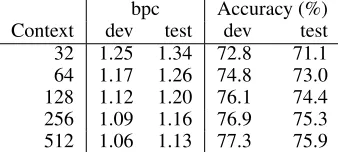
bpc Accuracy (%)

Context dev test dev test

32 1.25 1.34 72.8 71.1

64 1.17 1.26 74.8 73.0

128 1.12 1.20 76.1 74.4

256 1.09 1.16 76.9 75.3

512 1.06 1.13 77.3 75.9

Table 2: Bits per character (bpc) and accuracy of our best model ontext8dev and test, for different context lengths.

and a filter size of 2048. We feed our model sequences of length 512. Each item in the sequence represents a single byte (or equivalently, one character in text8) which gets replaced by its embedding, a vector of size 512. We add to the byte embeddings a separate learned positional embed-ding for each of the 512 token positions, as described in the Positional Embeddings section above. We do the same ad-dition at each layer activation throughout the network. The positional embeddings are not shared across the layers. With two predictions per position, each layer learns to predict 1024 characters. Because we are primarily interested in pre-dicting the immediately following character (one step away), we halve the loss of predicting characters two steps away. The prediction layers are logistic regression layers over the full 256 outputs (the number of unique bytes). To demon-strate the generality of the model, we always train and pre-dict over all 256 labels, even on datasets that cover a smaller vocabulary. Despite this, we found that in practice the model never predicted a byte value outside of the ones observed in the training dataset.

The model has approximately 235 million parameters, which is larger than the number of characters in thetext8

training corpus. To regularize the model, we apply dropout in the attention and ReLU layers with a probability of 0.55. We use the momentum optimizer with 0.99 momentum. The learning rate is fixed during training to 0.003. We train our model for 4 million steps, with each step processing a batch of 16 randomly selected sequences. We drop the intermedi-ate layer losses consecutively, as described in the Intermedi-ate Layer Losses section above. Starting from the first layer, after every62.5K (= 4M× 1

2∗64) steps, we drop the losses

(4)

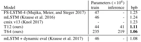
Parameters (×106₎

Model train inference bpb

FS-LSTM-4 (Mujika, Meier, and Steger 2017) 47 - 1.25 mLSTM (Krause et al. 2016) 46 - 1.24

cmix v13 (Knol 2017) - - 1.23

T12 (ours) 44 41 1.11

T64 (ours) 235 219 1.06

mLSTM + dynamic eval (Krause et al. 2017) 46 - 1.08

Table 3: Comparison of various models onenwik8test.

Evaluation

At inference time, we use the model’s prediction at the fi-nal position of the fifi-nal layer to compute the probability of a character given a context of 512 characters. There is no state passed between predictions as would be the case with RNN models, so for each character predicted we have to pro-cess the context from scratch. Because there is no reused computation from previous steps, our model requires ex-pensive computational resources for evaluation and infer-ence. We measure the performance of training checkpoints (roughly every 10,000 steps) by evaluating bits per character (bpc) over the entire the validation set, and save the param-eters that perform the best. Our best model is achieved after around 2.5 million steps of training, which takes 175 hours on a single Google Cloud TPU v2.

Results

We report the performance of our best model (T64) on the validation and test sets. Table 1 compares our models against several recent results. On the test set, we achieve a new state of the art, 1.13 bpc. This model is 5x larger than previous models, which necessitated aggressive dropout rates of 0.55. For better comparison with smaller models, we also train a smaller model (T12) with 41M parameters. This model con-sists of 12 layers, and trained for 8M steps, with a reduced dropout rate of 0.2. All other settings were left the same as T64. Our smaller model still outperforms previous models, achieving 1.18 bpc on the test dataset. Increasing the depth of the network from 12 layers to 64 improved the results sig-nificantly, with the auxiliary losses enabling the training to better utilize the depth of the network. Note, our models do not use dynamic evaluation (Krause et al. 2017), a technique that adjusts model weights at test time by training on test data.

Table 2 shows the performance of our model given differ-ent context sizes. We are able to achieve state-of-the-art re-sults once the context increases beyond 128 characters, with the best performance of 1.06 bpc at 512 characters. As ex-pected, the model performs better when it is given more con-text. However this trend levels off after 512 characters; we do not see better results using a context of 1024.

Using the same hyperparameters and training procedure fortext8, we also train and evaluate the T12 and T64 ar-chitectures onenwik8(see Table 3). Note, several previous authors discuss “bits per character” onenwik8but are in fact reporting bits per byte. Without retuning for this dataset, our models still achieve state-of-the-art performance.

Ablation Experiments

To better understand the relative importance of the several modifications we proposed, we run an ablation analysis. We start from our best model T64 and then remove one modifi-cation at a time. For example, when we disableMultiple Po-sitions, the model gets trained with only the last position loss for each layer. This corresponds to calculating{L(t4|t0:3),

L(t5|t0:3)}in the example shown in Figure 1d for both the

first and the second layers. When disablingPositional Em-beddings, we add the default transformer sinusoidal timing signal before the first layer.

Description bpc ∆bpc

T64 (Baseline) 1.062

-T64 w/out Multiple Positions 2.482 1.420

T64 w/out Intermediate Layer Losses 1.158 0.096 T64 w/out Positional Embeddings 1.069 0.007

T64 w/out Multiple Targets 1.068 0.006

T64 w/ SGD Optimizer 1.065 0.003

Table 4: Evaluation of T64 ontext8dev with context set to 512. Disabling each feature or loss lowers the quality of the model. The biggest win comes from adding multiple po-sitions and intermediate layers losses.

For the ablation experiments, we reuse the hyperparame-ters from our best model to avoid a prohibitively expensive parameter search for each ablation. The only exception is the SGD experiment, where we vary the learning rate. The analysis shows that the biggest advantage comes from mul-tiple positions and intermediate layers losses. Predicting all the intermediate positions leads to significant speed up in convergence, since the model sees more effective training examples per batch. Adding losses at the intermediate lay-ers acts in the same spirit by forcing more predictions per training step.

Finally, we replace momentum with SGD as our opti-mizer, using a range of learning rates (0.3, 0.1, 0.03, 0.01, 0.003, 0.001). This ablation shows that SGD produces com-petitive models, with learning rate 0.1 giving the best per-formance. Despite the depth of our network, SGD is able to train the network efficiently with the help of our auxiliary losses.

Comparison with Word-Level Models

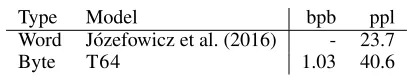
To understand how byte-level language models perform in comparison to word-level language models, we train T64 on the lm1b corpus (Chelba et al. 2013). For lm1b, we use the standard train/test split of the preprocessed corpus, where out-of-vocab words have been replaced withUNK, to allow comparison to previous work on word and word-piece models. We report word perplexity (ppl) by converting bits-per-byte (bpb) intoppl2. During training we use the sec-ond shard (01) of the heldout dataset as a dev set, as the first shard (00) is the test. Given this is a significantly larger dataset than text8, we set all dropouts to zero. Table 5

2

(5)

Type Model bpb ppl Word J´ozefowicz et al. (2016) - 23.7

Byte T64 1.03 40.6

Table 5: Performance of T64 on thelm1btest set.

Seed

mary was not permitted to see them or to speak in her own defence at the tribunal she refused to offer a written defence unless elizabeth would guarantee a verdict of not guilty which elizabeth would not do although the casket letters were ac-cepted by the inquiry as genuine after a study of the hand-writing and of the information contained therein and were generally held to be certain proof of guilt if authentic the in-quiry reached the conclusion that nothing was proven from the start this could have been pr

Word Completions

proven, proved, proof, prevented, presented, problematic, probably, provided, practical, provoked, preceded, predicted, previously, presumed, praised, proposed, practicable, pro-duced, present, preserved, precisely, prior, protected, prob-able, prompted, proofed, properly, practiced, prohibited, pro-found, preferable, proceeded, precise, predictable, practi-cally, prevalent

Figure 2: A seed sequence of 512 characters taken from the

text8test set, and all word completions assigned cumula-tive probability above 0.001 to follow the seed, in order from most likely (0.529) to least likely (0.001).

shows a gap in performance between the two classes of lan-guage models. This comparison can serve as a starting point for researching possible ways to bridge the gap.

Qualitative Analysis

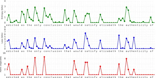
To probe the strengths and weaknesses of our best model (T64), we run the model forward, starting with the seed se-quence of 512 characters in Figure 2, taken from thetext8

test set. Figure 3 shows several per-character metrics for the model’s predictions over the true continuation of this seed text. At each position, we measure i) the model’s prediction entropy in bits across all 256 output classes, ii) its loss— the negative log probability of the target label, i.e. the “bits per character” for this position, and iii) the rank of the tar-get in the list of output classes sorted by likelihood. Unsur-prisingly, the model is least certain when predicting the first character of a word, and becomes progressively more confi-dent and correct as subsequent characters are seen.

To investigate the degree to which our model prefers ac-tual English words over non-existent words, we compute the likelihood the model assigns to all continuations after the seed. We cut off continuations when they reach a space char-acter, or when the total probability of the continuation falls below 0.001. Figure 2 shows the entire set of word comple-tions, in order of probability, where the initialpr-from the

seed is repeated for readability. Note that these are all real or plausible (proofed) English words, and that even short but bad continuations likeprzare assigned a lower cumu-lative probability than long realistic word completions like

predictable.

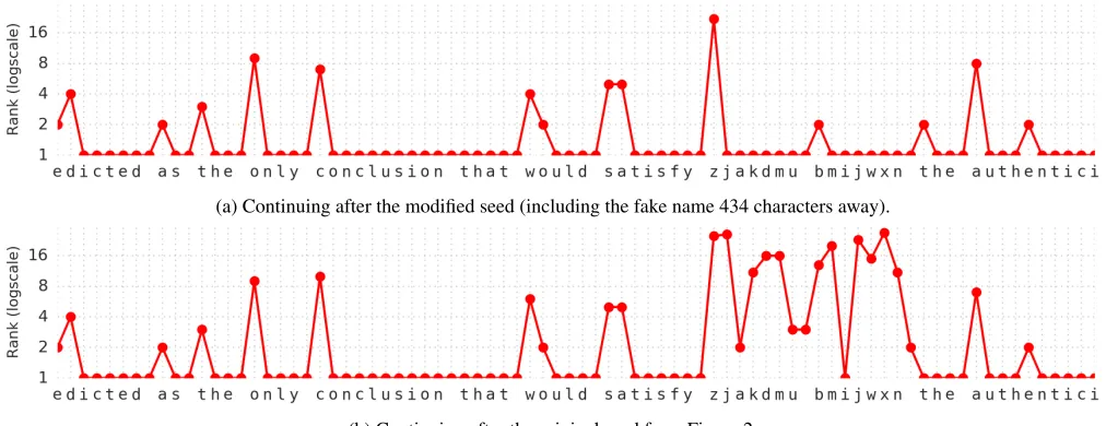
We expect that the transformer self-attention should make it easy for our model to copy sequences observed in the con-text over long distances (up to the concon-text size of 512 char-acters). To test this expectation, we corrupt the seed and con-tinuation from above by introducing a fake namezjakdmu bmijwxn. Specifically, we change the first occurrence of

elizabethin the seed tozjakdmu bmijwxn, and the second occurrence toshe. Similarly, in the continuation, we changeelizabethtozjakdmu bmijwxn. The result-ing distance between the two occurrences of the fake name is 434 characters.

Figure 4a confirms that the model can successfully copy over this long distance. While the initialzinzjakdmuis unexpected, the model immediately chooses to copy the re-mainder of this word from the context, as opposed to pre-dicting any realz-words learned during training. Similarly, while the model is somewhat unsure whether the fake sur-namebmijwxnwill appear (assigning the initialba rank of two), it immediately picks up on the correspondence after thebis observed, correctly predicting the remainder of the fake surname.

For comparison, Figure 4b shows how the model would rank the targets in our fake continuation if the original seed withelizabeth were used. This confirms that the fake name is not predictable based on knowledge gained through training, and is indeed being copied from the preceding con-text.

Generation

For generating samples using our language model, we train on a larger and less processed dataset,enwik9(Mahoney 2009). We split enwik9 into 900M, 50M and 50M for training, dev and test. Using the dev dataset to tune our dropout, we find that dropout=0.1 performs the best. On the test dataset, T64 achieves 0.85bpb. Table 6 shows different generated samples following the seed text, using a sampling temperature of 1.0.

Related Work

Character-level modeling has shown promise in many ar-eas such as sentiment analysis (Radford, J´ozefowicz, and Sutskever 2017), question answering (Kenter, Jones, and Hewlett 2018) and classification (Zhang, Zhao, and LeCun 2015), and is an exciting area due to its simplicity and the ability to easily adapt to other languages. Neural network based language modeling has been heavily researched since its effectiveness was shown by Bengio et al. (2003). By far, the most popular architecture in this area is the RNN and variants, first studied in Mikolov et al. (2010).

(6)

Figure 3: Per-character entropy, loss and rank assigned by T64 after seeding on the 512 character sequence from Figure 2.

Seed

'''Computational neuroscience''' is an interdisciplinary field which draws on [[neuroscience]], [[computer sci-ence]], and [[applied mathematics]]. It most often uses mathematical and computational techniques such as com-puter [[simulation]]s and [[mathematical model]]s to un-derstand the function of the [[nervous system]].

The field of computational neuroscience began with the work of [[Andrew Huxley]], [[Alan Hodgkin]], and [[David Marr]]. The results of Hodgkin and Huxley's pi-oneering work in developing

Sample 1 computational neuroscience were chronicled in ''[[Is Mathematics Anything I Could Learn?]]''. (ISBN 0826412246). Computational

Sample 2 neuroscience concerned neurological auraria and the inherited ability to communicate and respond to environmental destruction

-Sample 3 the model were published in 1982 and 1983 re-spectively, and the subsequent work on the field began its graduate program with [[M

Truth the voltage clamp allowed them to develop the first mathematical model of the [[action poten-tial]]. David Marr's work focuses on

Table 6: Samples generated by T64, seeded with text from theenwik9dev set, using a sampling temperature of 1.0.

Highway Networks (Zilly et al. 2016), Unitary RNNs (Ar-jovsky, Shah, and Bengio 2015) and others. This is an issue

that transformers do not have, due to attention allowing short paths to all inputs. Methods of normalizing activation func-tions, such as Batch Normalization (Ioffe and Szegedy 2015; Merity, Keskar, and Socher 2017) and Layer Normaliza-tion (Lei Ba, Kiros, and Hinton 2016) have also demon-strated improvements on language modeling tasks. As with this work, progress has been made with discovering ways to regularize sequential architectures, with techniques such as Recurrent Dropout (Zaremba, Sutskever, and Vinyals 2014; Gal and Ghahramani 2015) and Zoneout (Krueger et al. 2016; Rocki 2016).

A related architecture is the Neural Cache Model (Grave, Joulin, and Usunier 2016), where the RNN is allowed to at-tend to all of its previous hidden states at each step. An-other similar model is used in (Daniluk et al. 2017) where a key-value attention mechanism similar to transformers is used. Both approaches show improvements on word level language modeling. Memory Networks (Weston, Chopra, and Bordes 2014) have a similarity to the transformer model in design as it also has layers of attention for processing a fix memory representing the input document and has been shown to be effective for language modeling in (Sukhbaatar et al. 2015). ByteNet (Kalchbrenner et al. 2016), which is related but uses layers of dilated convolutions rather than attention, showed promising results on byte level language modeling. Gated Convolutional Networks (Dauphin et al. 2016) was an early non-recurrent model to show superior performance on word level language modeling.

(7)

(a) Continuing after the modified seed (including the fake name 434 characters away).

(b) Continuing after the original seed from Figure 2.

Figure 4: Per-character rank assigned by T64 to a fake continuation, after being seeded on either (a) the fake context where

elizabethis replaced withzjakdmu bmijwxn, or (b) the original context.

a large number of parameters. A recent CNN model for text classification (Conneau et al. 2016) at 29 layers is considered deep in the NLP community. A Sparsely-Gated Mixture-of-Experts Layer (Shazeer et al. 2017) allowed lan-guage modeling experiments with a greatly increased num-ber of parameters by only accessing a small portion of pa-rameters every time step, showing a reduction in bits per word. In J´ozefowicz et al. (2016), an increase in the num-ber of parameters was achieved by mixing character-level and word level models, using specialized softmaxes and us-ing a large amount of computational resources to train. In-dRNN (Li et al. 2018) uses a simplified RNN architecture that allows deeper stacking with 21-layers, achieving near SOTA character-level language modeling. Fast-Slow Recur-rent Neural Networks (Mujika, Meier, and Steger 2017) also achieved near SOTA by increasing the number of recurrent steps for each character processed.

Conclusion

Character language modeling has been dominated by re-current network approaches. In this paper, we show that a network of 12 stacked transformer layers achieves state-of-the-art results on this task. We gain further improvements in quality by deepening the network to 64 layers, utilizing capacity and depth efficiently. The use of auxiliary losses at intermediate layers and positions is critical for reaching this performance, and these losses allow us to train much deeper transformer networks. Finally, we analyze the behavior of our network and find that it is able to exploit dependencies in structure and content over long distances, over 400 char-acters apart.

References

Arjovsky, M.; Shah, A.; and Bengio, Y. 2015. Unitary evo-lution recurrent neural networks.CoRRabs/1511.06464.

Bengio, Y.; Ducharme, R.; Vincent, P.; and Janvin, C. 2003. A neural probabilistic language model.J. Mach. Learn. Res.

3:1137–1155.

Chelba, C.; Mikolov, T.; Schuster, M.; Ge, Q.; Brants, T.; Koehn, P.; and Robinson, T. 2013. One billion word bench-mark for measuring progress in statistical language model-ing.arXiv preprint arXiv:1312.3005.

Cho, K.; van Merrienboer, B.; Gülçehre, Ç .; Bougares, F.; Schwenk, H.; and Bengio, Y. 2014. Learning phrase rep-resentations using RNN encoder-decoder for statistical ma-chine translation. CoRRabs/1406.1078.

Chung, J.; Ahn, S.; and Bengio, Y. 2016. Hierarchi-cal multisHierarchi-cale recurrent neural networks. arXiv preprint

arXiv:1609.01704.

Chung, J.; Gulcehre, C.; Cho, K.; and Bengio, Y. 2015. Gated feedback recurrent neural networks. InInternational

Conference on Machine Learning, 2067–2075.

Conneau, A.; Schwenk, H.; Barrault, L.; and LeCun, Y. 2016. Very deep convolutional networks for natural lan-guage processing. CoRRabs/1606.01781.

Cooijmans, T.; Ballas, N.; Laurent, C.; and Courville, A. C. 2016. Recurrent batch normalization. CoRR

abs/1603.09025.

Daniluk, M.; Rockt¨aschel, T.; Welbl, J.; and Riedel, S. 2017. Frustratingly short attention spans in neural language mod-eling.CoRRabs/1702.04521.

Dauphin, Y. N.; Fan, A.; Auli, M.; and Grangier, D. 2016. Language modeling with gated convolutional networks.

CoRRabs/1612.08083.

Gal, Y., and Ghahramani, Z. 2015. A Theoretically Grounded Application of Dropout in Recurrent Neural Net-works. ArXiv e-prints.

(8)

neural language models with a continuous cache. CoRR

abs/1612.04426.

Hochreiter, S., and Schmidhuber, J. 1997. Long short-term memory. InNeural computation, volume 9, 1735–80. Hochreiter, S.; Bengio, Y.; Frasconi, P.; Schmidhuber, J.; et al. 2001. Gradient flow in recurrent nets: the difficulty of learning long-term dependencies.

Ioffe, S., and Szegedy, C. 2015. Batch normalization: Accel-erating deep network training by reducing internal covariate shift. CoRRabs/1502.03167.

J´ozefowicz, R.; Vinyals, O.; Schuster, M.; Shazeer, N.; and Wu, Y. 2016. Exploring the limits of language modeling.

CoRRabs/1602.02410.

Kalchbrenner, N.; Espeholt, L.; Simonyan, K.; Oord, A. v. d.; Graves, A.; and Kavukcuoglu, K. 2016. Neu-ral machine translation in linear time. arXiv preprint

arXiv:1610.10099.

Ke, N. R.; Goyal, A.; Bilaniuk, O.; Binas, J.; Charlin, L.; Pal, C.; and Bengio, Y. 2017. Sparse attentive backtracking: Long-range credit assignment in recurrent networks. arXiv preprint arXiv:1711.02326.

Kenter, T.; Jones, L.; and Hewlett, D. 2018. Byte-level ma-chine reading across morphologically varied languages. Khandelwal, U.; He, H.; Qi, P.; and Jurafsky, D. 2018. Sharp nearby, fuzzy far away: How neural language models use context. InAssociation for Computational Linguistics (ACL).

Knol, B. 2017. cmix - byronknoll.com/cmix.html.

Krause, B.; Lu, L.; Murray, I.; and Renals, S. 2016. Mul-tiplicative lstm for sequence modelling. arXiv preprint

arXiv:1609.07959.

Krause, B.; Kahembwe, E.; Murray, I.; and Renals, S. 2017. Dynamic evaluation of neural sequence models. arXiv preprint arXiv:1709.07432.

Krueger, D.; Maharaj, T.; Kram´ar, J.; Pezeshki, M.; Ballas, N.; Ke, N. R.; Goyal, A.; Bengio, Y.; Courville, A.; and Pal, C. 2016. Zoneout: Regularizing rnns by randomly preserv-ing hidden activations.arXiv preprint arXiv:1606.01305. Lei Ba, J.; Kiros, J. R.; and Hinton, G. E. 2016. Layer Normalization.ArXiv e-prints.

Li, S.; Li, W.; Cook, C.; Zhu, C.; and Gao, Y. 2018. In-dependently recurrent neural network (indrnn): Building A longer and deeper RNN.CoRRabs/1803.04831.

Mahoney, M. 2009. Large text compression benchmark. http://www.mattmahoney.net/text/text.html.

Merity, S.; Keskar, N. S.; and Socher, R. 2017. Reg-ularizing and optimizing LSTM language models. CoRR

abs/1708.02182.

Mikolov, T.; Karafi´at, M.; Burget, L.; Cernock´y, J.; and Khu-danpur, S. 2010. Recurrent neural network based language model. In Kobayashi, T.; Hirose, K.; and Nakamura, S., eds.,

INTERSPEECH, 1045–1048. ISCA.

Mikolov, T.; Kombrink, S.; Burget, L.; ˇCernock´y, J.; and Khudanpur, S. 2011. Extensions of recurrent neural

net-work language model. In2011 IEEE International Confer-ence on Acoustics, Speech and Signal Processing (ICASSP), 5528–5531.

Mikolov, T.; Sutskever, I.; Deoras, A.; Le, H.-S.; Kombrink, S.; and Cernocky, J. 2012. Subword language model-ing with neural networks. preprint (http://www. fit. vutbr. cz/imikolov/rnnlm/char. pdf)8.

Mujika, A.; Meier, F.; and Steger, A. 2017. Fast-slow re-current neural networks. InAdvances in Neural Information

Processing Systems, 5915–5924.

Radford, A.; J´ozefowicz, R.; and Sutskever, I. 2017. Learn-ing to generate reviews and discoverLearn-ing sentiment. CoRR

abs/1704.01444.

Rocki, K. M. 2016. Surprisal-driven feedback in recurrent networks. arXiv preprint arXiv:1608.06027.

Salimans, T.; Zhang, H.; Radford, A.; and Metaxas, D. N. 2018. Improving gans using optimal transport. CoRR

abs/1803.05573.

Shazeer, N.; Mirhoseini, A.; Maziarz, K.; Davis, A.; Le, Q. V.; Hinton, G. E.; and Dean, J. 2017. Outra-geously large neural networks: The sparsely-gated mixture-of-experts layer. CoRRabs/1701.06538.

Sukhbaatar, S.; Weston, J.; Fergus, R.; et al. 2015. End-to-end memory networks. InAdvances in neural information

processing systems, 2440–2448.

Sundermeyer, M.; Schl¨uter, R.; and Ney, H. 2012. Lstm neural networks for language modeling. InThirteenth an-nual conference of the international speech communication association.

Tallec, C., and Ollivier, Y. 2017. Unbiasing truncated back-propagation through time.arXiv preprint arXiv:1705.08209. Vaswani, A.; Shazeer, N.; Parmar, N.; Uszkoreit, J.; Jones, L.; Gomez, A. N.; Kaiser, L.; and Polosukhin, I. 2017. At-tention is all you need. InAdvances in Neural Information Processing Systems 30. Curran Associates, Inc. 5998–6008. Werbos, P. J. 1990. Backpropagation through time: what it does and how to do it. Proceedings of the IEEE

78(10):1550–1560.

Weston, J.; Chopra, S.; and Bordes, A. 2014. Memory net-works. CoRRabs/1410.3916.

Zaremba, W.; Sutskever, I.; and Vinyals, O. 2014. Recurrent neural network regularization. CoRRabs/1409.2329. Zhang, S.; Wu, Y.; Che, T.; Lin, Z.; Memisevic, R.; Salakhutdinov, R. R.; and Bengio, Y. 2016. Architectural complexity measures of recurrent neural networks. In

Ad-vances in Neural Information Processing Systems, 1822–

1830.

Zhang, X.; Zhao, J. J.; and LeCun, Y. 2015. Character-level convolutional networks for text classification. CoRR

abs/1509.01626.

Zilly, J. G.; Srivastava, R. K.; Koutn´ık, J.; and Schmid-huber, J. 2016. Recurrent highway networks. CoRR