Streaming kernel regression with provably adaptive
mean, variance, and regularization
Audrey Durand [email protected]
Universit´e Laval, Qu´ebec, Canada
Odalric-Ambrym Maillard [email protected]
INRIA, Lille, France
Joelle Pineau [email protected]
McGill University & Facebook AI Research, Montreal, Canada
Editor:Csaba Szepesvari
Abstract
We consider the problem of streaming kernel regression, when the observations arrive se-quentially and the goal is to recover the underlying mean function, assumed to belong to an RKHS. The variance of the noise is not assumed to be known. In this context, we tackle the problem of tuning the regularization parameter adaptively at each time step, while maintaining tight confidence bounds estimates on the value of the mean function at each point. To this end, we first generalize existing results for finite-dimensional linear regres-sion with fixed regularization and known variance to the kernel setup with a regularization parameter allowed to be a measurable function of past observations. Then, using appropri-ate self-normalized inequalities we build upper and lower bound estimappropri-ates for the variance, leading to Bernstein-like concentration bounds. The latter is used in order to define the adaptive regularization. The bounds resulting from our technique are valid uniformly over all observation points and all time steps, and are compared against the literature with numerical experiments. Finally, the potential of these tools is illustrated by an application to kernelized bandits, where we revisit the Kernel UCB and Kernel Thompson Sampling procedures, and show the benefits of the novel adaptive kernel tuning strategy.
Keywords: kernel, regression, online learning, adaptive tuning, bandits
1. Introduction
Many applications require solving an online optimization problem for an unknown, noisy, function defined over a possibly large domain space. Kernel regression methods can learn such possibly non-linear functions by sharing information gathered across observations. These techniques are being used in many fields where they serve a variety of applications like hyperparameters optimization (Snoek et al., 2012), active preference learning (Brochu et al., 2008), and reinforcement learning (Marchant and Ramos, 2014; Wilson et al., 2014). The idea is generally to rely on kernel regression to estimate a function that can be used for decision making and selecting the next observation point. Algorithmically speaking, standard kernel regression involves a regularization parameter that accounts for both the complexity of the unknown target function, and the variance of the noise. While most
c
theoretical approaches rely on a fixed regularization parameter, in practice, people have often used heuristics in order to tune this parameter adaptively with time.
This however comes at the price of loosing theoretical guarantees. Indeed, in or-der for theoretical guarantees (based on concentration inequalities) to hold, existing ap-proaches (Srinivas et al., 2010; Valko et al., 2013) require the regularization parameter in the kernel regression to be a fixed quantity. Further, they assume a prior and tight knowledge of the variance of the noise, which is unrealistic in practice. The reason for this cumbersome assumption is to adjust the regularization parameter in the kernel regression based on this deterministic quantity, as such a choice of regularization conveys a natural Bayesian interpretation (Rasmussen and Williams, 2006). Following this intuition, given an empirical estimate of the function noise based on gathered observations, one should be able to tune the regularization automatically. This is however non-trivial, first due to the streaming nature of the data, that allows the noise to be a measurable function of the past observations, second because concentration bounds on the empirical variance are currently unknown in such a general kernel setup, and finally because all existing theoretical bounds require the regularization parameter to be a deterministic constant, while we require here a parameterization that explicitly depends on past observations. The goal of this work is to provide the rigorous tools for performing an online tuning of the kernel regularization while preserving theoretical guarantees and confidence intervals in the context of stream-ing kernel regression with unknown noise. We thus hope to provide a sound method for adaptive tuning that is both interesting from a practical perspective and retains theoretical guarantees.
We gently start our contributions by Theorem 1 that generalizes existing concentration results (such as in Abbasi-Yadkori et al. (2011); Wang and de Freitas (2014)), and is explic-itly stated for a regularization parameter that may differ from the noise. This result paves the way to an even more general result (Theorem 2) that holds when the regularization is tuned online at each step. Afterwards, we introduce a streaming variance estimator (The-orem 3) that yields empirical upper- and lower-bounds on the function noise. Plugging-in the resulting estimates leads to empirical Bernstein-like concentration results (Corollary 1) for the kernel regression, where we use the variance estimates in order to tune the regu-larization parameter. Section 4 presents an application to kernelized bandits, where regret bounds for Kernel UCB and Kernel Thompson Sampling procedures are derived. Section 5 discusses our results and compares them against other approaches. Finally, Section 6 shows the potential of all the previously introduced results while comparing them to existing al-ternatives through different numerical experiments. We postpone most of the proofs to the appendix.
2. Kernel streaming regression with a predictable noise process
Let us consider a sequential regression problem. At each time step t∈N, a learner picks a point xt∈ X ⊂Rd and gets the observation
yt=f?(xt) +ξt,
wheref? is an unknown function assumed to belong to some function space F, andξt is a
Assumption 1 (Predictability) The process generating the observations is predictable
in the sense that there is a filtration H= (Ht)t∈N such that xt is Ht−1-measurable and yt
is Ht-measurable. Such an example is given byHt=σ(x1, . . . , xt+1, y1, . . . , yt).
Assumption 2 (Sub-Gaussian streaming model) In the sub-Gaussian streaming pre-dictable model, for some non-negative constant σ2, the following holds
∀t∈N,∀γ ∈R, lnE
h
exp(γξt)
Ht−1
i 6 γ
2σ2 2 .
Letk:X × X →Rbe a kernel function (that is continuous, symmetric positive definite) on a compact set X equipped with a positive finite Borel measure, and denote K the corresponding RKHS.
Information gain This quantity measures the information obtained about function f?
by sampling at points (x1, . . . , xt). It is defined (Cover and Thomas, 1991) as the mutual information betweenf? and the observations (y1, . . . , yt):
I(y1, . . . , yt;f?) =H(y1, . . . , yt)−H(y1, . . . , yt|f?),
that is the difference between the marginal entropy and the conditional entropy of the distributions of observations. The information gain thus quantifies the reduction of uncer-tainty about f? following these observations. For a multidimensional Gaussian, we have
H(N(µ,Σ)) = 12ln|2πeΣ|, such that forλ=σ2 (Srinivas et al., 2010),
γt(σ2) =I(y1, . . . , yt;f?) =
1
2ln det(It+σ
−2K
t),
where Kt = (k(s, s0))s,s06t. In the linear case when k(x, x0) = x>x0 for x ∈Rd, the infor-mation gain typically scales as γt(σ2) = O(dlnt) (Srinivas et al., 2010). The information
gain can be shown to scale with the effective dimensionality (Valko et al., 2013) instead of the dimension, where effective dimensions correspond to the most informative ones. More effective dimensions require more observations for a good space coverage, which increases the information gain. We now extend the information gain to any regularizationλ.
Definition 1 (Information gain with unknown variance) We define the information gain at time t for a regularization parameterλ to be
γt(λ) =
1 2
t
X
t0=1
ln1 +1
λkλ,t0−1(xt0, xt0)
.
Concentration We first provide a result bounding the prediction error of a standard regularized kernel estimate, where the regularization is given by a fixed parameter λ >0.
Theorem 1 (Streaming kernel least-squares (Maillard, 2016)) Assume we are in the sub-Gaussian streaming predictable model. For a parameterλ∈R, let us define the posterior
mean and variances after observing Yt= (y1, . . . , yt)>∈Rt×1 as
(
fλ,t(x) = kt(x)>(Kt+λIt)−1Yt
s2
λ,t(x) = σ
2
λkλ,t(x, x) with kλ,t(x, x) =k(x, x)−kt(x) >(K
t+λIt)−1kt(x).
where kt(x) = (k(x, xt0))t06t is a t×1 (column) vector and Kt = (k(xs, xs0))s,s06t. Then
∀δ∈[0,1], with probability higher than 1−δ, it holds simultaneously over allx∈X and t>0,
|f?(x)−fλ,t(x)|6
r
kλ,t(x, x)
λ √
λkf?kK+σ
p
2 ln(1/δ) + 2γt(λ)
,
where the quantity γt(λ) = 12Ptt0=1ln
1+λ1kλ,t0−1(xt0, xt0)
is the information gain.
Remark 1 This result should be considered as an extension of Abbasi-Yadkori et al. (2011, Theorem 2) from finite-dimensional to possibly infinite dimensional function space. More specifically, when considering the linear kernel, the result of Theorem 1 recovers exactly Theorem 2 from Abbasi-Yadkori et al. (2011). The generalization is non trivial as the Laplace method must be amended in order to be applied beyond the linear case.
Remark 2 This result holds uniformly over allx∈ X and most importantly over allt>0, thanks to a random stopping time construction (related to the occurrence of bad events) and a self-normalized inequality handling this stopping time. This is in contrast with results such as Wang and de Freitas (2014), that are only stated separately for each t.
The case whenλ=λ?
def = σ2/kf
?k2K is of special interest, since we get on the one hand
fλ?,t(x) = kt(x)
>(K
t+λ?It)−1Yt
s2λ?,t(x) = kf?k2Kkt(x, x) withkt(x, x) =k(x, x)−kt(x)>(Kt+λ?It)−1kt(x)
and on the other hand
|f?(x)−fλ?,t(x)|6kf?kK
p
kt(x, x)
h
1 +p2 ln(1/δ) + 2γt(λ?)
i .
In practice however, neither kf?k2K nor σ2 may be known exactly. In this paper, we make
the following assumption on the former:
Assumption 3 (Bounded norm in RKHS) An upper boundC is given onkf?kK. This essentially means that the kernel is well chosen for capturingf?. For more details, see Canu et al. (2009); Loustau (2009); Wasserman (2017).
Theorem 2 (Streaming kernel least-squares with online tuning) Under the same as-sumption as Theorem 1, let λ = (λt)t>1 be a predictable positive sequence of parameters,
that is λt is Ht−1-measurable for each t. Assume that for each t, λt>λ? holds for a pos-itive constant λ?. Let us define the modified posterior mean and variances after observing
Yt∈Rt as
(
fλ,t(x) =kt(x)>(Kt+λt+1It)−1Yt
s2
λ,t(x) = σ
2
λt+1kλt+1,t(x, x)with kλ,t(x, x) =k(x, x)−kt(x)
>(K
t+λIt)−1kt(x),
where kt(x) = (k(x, xt0))t06t, and Kt= (k(xs, xs0))s,s06t. Then for allδ∈[0,1], with
probabil-ity higher than 1−δ, it holds simultaneously over all x∈ X andt>0
|f?(x)−fλ,t(x)|6
s
kλt+1,t(x, x)
λt+1
hp
λt+1kf?kK+σ
p
2 ln(1/δ)+2γt(λ?)
i .
The proof is presented in Appendix A.
The regularization parameter λt+1 is therefore used in conjunction with previous data up to timet to provide the posterior regression model (mean and variance) that is used in return to acquire the next observation yt+1 on pointxt+1.
Remark 3 Since λt is allowed to be Ht−1-measurable, this gives theoretical guarantees for
virtually any adaptive tuning procedure of the regularization parameter.
Remark 4 The assumption that λt >λ? will be naturally satisfied for the choice of regu-larization we consider.
3. Variance estimation
We now focus on the estimation of the variance parameter of the noise in the case when it is unknown, or loosely known. Theorem 2 suggests to define the sequence (λt)t>1 by
λt=σ2+,t−1/C2 with σ+,t= min{σ˜+,t, σ+,t−1} and σ+,0 =σ+, (1) where σ+ > σ is an initial loose upper bound on σ and ˜σ+,t is an upper-bound estimate
on σ built from all observations gathered up to time t (inclusively). This ensures that λt
isHt−1 measurable for allt and satisfiesλt>λ? with high probability, where λ? =σ2/C2.
The crux is now to define the upper-bound estimate σ+,t on σ. In order to get a variance
estimate, one obviously requires more than the sub-Gaussian assumption, since the termσ2 has no reason to be tight (the inequality remains valid whenσ2 is replaced with any larger value). In order to convey the minimality ofσ2, we assume that the noise sequence is both
σ-sub-Gaussian and second-order1 σ-sub-Gaussian, in the sense that ∀t,∀γ < 1
2σ2 lnE
exp(γξt2)
Ht−1
6−1 2ln
1−2γσ2.
Remark 5 To avoid any technicality, one may assume thatξt|Ht−1 is exactlyN(0, σ2), in
which case it is trivially second-order σ-sub-Gaussian.
Now let bσ2
λ,T = T1
PT
t=1(yt−fλ,T(xt))2 denote the (slightly biased) variance estimate
for a regularization parameter λ.
Theorem 3 (Streaming kernel variance estimate) Assume we are in the predictable second-order σ-sub-Gaussian streaming regression model, with a predictable positive se-quence λ such that λt>λ? holds for allt. Let us introduce the following quantities
Ct(δ) = ln(e/δ)
1 + ln(π2ln(t)/6)/ln(1/δ)
, Dλ,t(δ) = 2 ln(1/δ) + 2γt(λ)
and finally α= max1−
q
Ct(δ0)
t −
q
Ct(δ0)+2Dλ?,t(δ0)
t ,0
.
Then, let us introduce the following variance bounds, defined differently depending on whether a deterministic upper bound σ+>σ is known (case 1) or not (case 2).
σ+,t(λ, λ?) =
b
σλ,t+σ+
q
Ct(δ0)
t +
q
Ct(δ0)+2Dλ?,t(δ0) t
+
q
2σ+kf?kK√λDλ?,t(δ0)
t (case 1)
1
α2
q
b σλ,tα+
kf?kK√λDλ?,t(δ0)
2t +
q
kf?kK√λDλ?,t(δ0) 2t
!2
(case 2)
σ−,t(λ) =
b
σλ,t−σ+
q
2Ct(δ0)
t − kf?kK
s
λ t
1− 1
maxt06t(1+λ1kλ,t0−1(xt0,xt0))
(case 1)
b
σλ,t− kf?kK
s
λ t
1− 1
maxt06t(1+λ1kλ,t0−1(xt0,xt0))
1 +
q
2Ct(δ0) t
−1
(case 2).
Then with probability higher than 1−3δ0, it holds simultaneously for all t>0
σ−,t(λt)6σ 6σ+,t(λt, λ?). The proof is presented in Appendix B.
Remark 6 The case when absolutely no bound is known on the noise σ2 is challenging in
practice. In this case, it is intuitive that one should not be able to recover the noise with too few samples. The bound stated in Theorem 3 (see Appendix B) supports this intuition, as when the number of observations is too small, then α = 0 and the corresponding bound becomes trivial (σ6∞).
Remark 7 In the variance bounds of Theorem 6 the term kf?kK appears systematically with the factor √λ. This suggests we need to chooseλproportional to1/kf?k2K, which gives further justification to the target λ? =σ2/C2, where C is a known upper bound on kf?k.
Remark 8 In practice, we advice to choose the best of case 1 and case 2 bounds when
Because λ? is not known in practice, the quantity σ+,t(λt, λ?) is not computable
di-rectly. However, we observe that σ+,t(λt, λ?) scales with Dλ?,t (directly and through α), and that Dλ?,t scales with the information gain γt(λ?). Recall that the information gain scales inversely with the regularization. Hence we have that for anyλ−6λ?, we also have
σ+,t(λ, λ−)>σ+,t(λ, λ?). Therefore, in order toestimate the upper bound σ+,t(λ, λ?), one
only needs a lower-bound onλ?. Let us define
σ−,t = max{σ˜−,t, σ−,t−1} with σ−,0=σ−, (2)
where 0 6 σ− 6σ is a initial lower-bound on σ and ˜σ−,t is a lower-bound estimate on σ
built from all observations gathered up to time t (inclusively). Then, one way to proceed is, at each time step t > 1, to build an estimate ˜σ−,t = σ−,t(λ), which in return can be
used to compute the lower quantity λ−=σ−2,t/C2 6σ2/C2 =λ?, and obtain the estimate
˜
σ+,t =σ+,t(λ, λ−)>σ+,t(λ, λ?). This “sandwich estimates” procedure allows us to build an
upper bound without prior knowledge ofλ?, and then compute the predictable sequenceλ
as described by Equation 1. Given Theorem 3, we have thatσ−,t(λt)6σsuch thatλ−6λ?
and σ+,t(λt, λ−) > σ, hence λt > λ?, simultaneously for all t > 0, with high probability.
Further replacing the variance σ with its estimate σ+,t using a union bound in the result
of Theorem 2, we derive confidence bounds that are fully computable empirically in the context where the regularization parameter is adaptively tuned and the function noise is unknown. This is summarized in the following empirical Bernstein-style inequality:
Corollary 1 (Kernel empirical-Bernstein inequality) Assume that C > kf?kK. Let us define the following noise lower-bound for each t>1
σ−,t = max{σ−,t(λt−1), σ−,t−1}
and define λ− =σ−2,t/C2 as the corresponding lower bound on λ?. Then, let us define the following noise upper bound for each t>1
σ+,t= min{σ+,t(λt−1, λ−), σ+,t−1}.
Define the regularization parameterizing the regression model used for acquiring observation at time t to be λt = σ+2,t/C2, according to Equation 1. Then with probability higher than
1−4δ, the following is valid simultaneously for all x∈ X and t>0,
f?(x)−fλt,t(x)
6
s
kλt,t(x, x)
λt
Bλt,t(δ) where
Bλt,t(δ) =
p
λtC+σ+,t
p
2 ln(1/δ) + 2γt(λ−). (3)
Proof Let Ef denote the event that
|f?(x)−fλ,t(x)|6
s
kλt+1,t(x, x)
λt+1
hp
λt+1kf?kK+σ
p
2 ln(1/δ)+2γt(λ?)
i
simultaneously for all x∈ X andt>0, and let Eλdenote the event that λt>λ? holds for
all t. We can decompose
By Theorem 2, we have thatP[Efc∩Eλ]6δ. We need to show thatλt>λ? for allt>0 by
tuningλtwith the proposed procedure. Let us look at what happens at each time t. Using
the proposed procedure, we haveλ0=σ+2/C2>λ?. Then we have
σ−,1(λ0)6σ L1
σ+,1(λ0, σ−,1(λ0)2/C2)>σ U1 →λ1 =σ+,1(λ0, σ−,1(λ0)2/C2)2/C2 >λ?
σ−,2(λ1)6σ L2
σ+,2(λ1, σ−,2(λ1)2/C2)>σ U2 →λ2 =σ+,2(λ1, σ−,1(λ1)2/C2)2/C2 >λ?
. . .
such that Eλ holds given that steps L1, U1, L2, U2, . . . hold simultaneously. Therefore,
P[Eλc] is bounded by the probability that these steps do not hold simultaneously. Following
Theorem 3, we have thatP[Eλc]63δ and thus P[Efc]64δ. Naturally, under the eventEλ,
we have σ+,t>σ and λ− 6λ?. Therefore, givenC>kf?kK, we have
p
λt+1kf?kK+σ
p
2 ln(1/δ) + 2γt(λ?)6
p
λt+1C+σ+,t
p
2 ln(1/δ) + 2γt(λ−).
Remark 9 This result is especially interesting since it provides a fully empirical confidence envelope function aroundf?. When an initial bound on the noiseσ+is known and considered
to be tight, one may simply choose the constant deterministic sequence λ = (λ, . . . , λ), in which case the same result holds for λ−=λand σ+,t=σ+.
We observe from Theorem 3 that the tightness of the noise estimates depends on theλ
parameter that is used for computing ˜σ−,t and ˜σ+,t. Sinceσ2/C2 6λt6σ+2/C2 holds with high probability by construction, using such an adaptive λt should yield tighter bounds
than using a fixedσ2
+/C2. This is supported by the numerical experiments of Section 6.2. 4. Application to kernelized bandits
Here is a direct application of our results in the framework of stochastic multi-armed bandits with structured arms embedded in an RKHS (Srinivas et al., 2010; Valko et al., 2013). At each time stept>1, a bandit algorithm recommends a pointxtto sample from a compact
set X ⊆ X, and observes a noisy outcome yt = f?(xt) +ξt, where ξt ∼ N(0, σ2). Let
x? = argmaxx∈Xf?(x) denote the optimal arm. The goal of an algorithm is to pick a sequence of points (xt)t6T that minimizes the cumulative regret
RT =
T
X
t=1
In this context, one needs to build tight confidence sets on the mean of each arm, and this will be given by Corollary 1. We illustrate our technique on two main bandit strategies: Upper Confidence Bound (UCB) (Auer et al., 2002) and Thompson Sampling (TS) (Thompson, 1933); both are adapted here to the kernel setting with unknown variance.
The following extension of Lemma 7 from Wang and de Freitas (2014) (see also Srinivas et al. (2012)) to the case when the variance is estimated plays an important role in the regret analysis of both algorithms.
Lemma 1 (From sum of variances to information gain) Let us assume that the ker-nel is bounded by 1 in the sense that supx∈Xk(x, x) 6 1. Let λ be any sequence such that ∀λ ∈ λ, λ > σ2/C2. For instance, this is satisfied with high probability when using
Equation 1. Then, it holds
T
X
t=1
s2λ,t−1(xt) =σ2 T
X
t=1 1
λt
kλt,t−1(xt, xt)6
2C2
ln(1 +C2/σ2)γT(σ 2/C2).
In the sequel, it is useful to bound the confidence bound termBλt,t(δ) from Equation 3.
Lemma 2 (Deterministic bound on the confidence bound) Assume that we are given a constant 0< σ−< σ, so thatσt,−>σ− holds for allt. Then for allt6T, the confidence bound term is upper-bounded by the following deterministic quantity
Bλt,t(δ)6σ+
1 +
q
2 ln(1/δ) + 2γT(σ−2/C2)
.
Further, we have γt(σ2t,−/C2) =γt(σ−2/C2) +O(1/
√
t).
Remark 10 The termσ+ can be replaced with a more refined termσ+O(1/ √
t) thanks to the confidence bounds on the variance estimates.
Kernel UCB with unknown variance The upper bound on the error can be used directly in order to build a UCB-style algorithm. Formally, the vanilla UCB algorithm (Auer et al., 2002) corresponding to our setting picks at timet the arm
xt∈argmax x∈X
fλ+t,t−1(x) where fλ,t+(x) =fλ,t(x) +
r
kλ,t(x, x)
λ Bλ,t(δ). (5)
Following the regret proof strategy of Abbasi-Yadkori et al. (2011), with some minor mod-ifications, yields the following guarantee on the regret of this strategy:
Theorem 4 (Kernel UCB with unknown noise and adaptive regularization) With probability higher than1−δ, the regret of Kernel UCB with adaptive regularization and vari-ance estimation satisfies for all T >0 (recall that Bλt+1,t(δ) is defined in Equation 3):
RT 62
T
X
t=1
s
kλt,t−1(xt, xt)
λt
Bλt,t−1(δ/4).
In particular, we have
RT 6 2σ+
σ
1 +
q
2 ln(4/δ) + 2γT(σ2−/C2)
C
s
T 2γT(σ2/C2)
Remark 11 This result that holds simultaneously over all time horizonT extends that of Abbasi-Yadkori et al. (2011) first to kernel regression and then to the case when the variance of the noise is unknown. This should also be compared to Valko et al. (2013) that assumes bounded observations, which implies a bounded noise (with known bound) and a boundedf?, and Srinivas et al. (2010) that provides looser bounds.
Kernel TS with unknown variance Another application of our confidence bounds is in the analysis of Thompson sampling in the kernel scenario. Before presenting the result, let us say a few words about the design of TS algorithm in a kernel setting. Such an algorithm requires sampling from a posterior distribution over the arms. It is natural to consider a Gaussian posterior with posterior means and variances given by the kernel estimates. However, it has been noted in a series of papers (Agrawal and Goyal, 2013; Abeille and Lazaric, 2017) that, in order to obtain provable regret minimization guarantees, the posterior variance should be inflated (although in practice, the vanilla version without inflation may work better). Following these lines of research, and owing to our novel confidence bounds, we derive the following TS algorithm using a posterior variance inflation factorv2
t.
Algorithm 1 Kernel TS with adaptive variance estimation and regularization tuning. Input: discrete spaceX.
Parameters: regularization sequenceλ, variance inflation factor v2
t for each t. 1: for allt>1do
2: compute the posterior meanbft−1 = (fλt,t−1(x))x∈X
3: compute the posterior covariance Σbt−1=
σ2 +,t−1
λt kλt,t−1(x, x
0)
x,x0∈
X
4: sample ˜ft=N(bft−1, v2tΣbt−1)
5: play xt= argmaxx∈Xf˜t(x) 6: observe outcome yt=f?(xt) +ξt
7: end for
Remark 12 The algorithm does not know the varianceσ2 of the noise, but uses an upper
estimate σ2 +,t−1.
Remark 13 We assume that the set of arms X is discrete. This is merely for
practi-cal reasons since otherwise updating the estimate of f? in a RKHS requires memory and computational times that are unbounded with t. This also simplifies the analysis.
The following regret bound can then be obtained after some careful but easy adaptation of Agrawal and Goyal (2013). We provide the proof of this result in Appendix C, which can be of independent interest, being a more rigorous and somewhat simpler rewriting of the original proof technique from Agrawal and Goyal (2013).
Theorem 5 (Regularized Kernel TS with variance estimate) Assume that the max-imal instantaneous pseudo-regret R= maxx∈X f?(x?)−f?(x)
is finite. Then, the regret of
Kernel TS (Algorithm 1) withvt=
Bλt,t−1(δ/4)
σ+,t−1 afterT episodes isO(C
p
with probability 1−3δ. More precisely, with probability 1−3δ, the regret is bounded for all
T >0:
RT 6 C1,T
T
X
t=1
s
kλt,t−1(xt, xt)
λt
Bλt,t−1(δ/4)
+C2R
p
Tln(1/δ) + 4πeRδ ,
where C1,T = (4√πe+ 1)
1 +
r
2 lnT(T√+1)|X|
πδ
and C2 =
q
8πe(1 +δ√4πe)2.
Further, we have
RT 6 C1,T
σ+
σ
1 +
q
2 ln(4/δ) + 2γT(σ−2/C2)
C
s
T 2γT(σ
2/C2) ln(1 +C2/σ2) +C2R
p
Tln(1/δ) + 4πeRδ .
Remark 14 As our confidence intervals do not require a bounded noise, likewise we can control the regret with high probability without requiring bounded observations, contrary to earlier works such as Valko et al. (2013).
5. Discussion and related works
Concentration results Theorem 1 extends the self-normalized bounds of Abbasi-Yadkori et al. (2011) from the setting of linear function spaces to that of an RKHS with sub-Gaussian noise. Based on a nontrivial adaptation of the Laplace method, it yields self-normalized inequalities in a setting of possibly infinite dimension. It generalizes the following result of Wang and de Freitas (2014) to kernel regression with λ6= σ2, which was already a gener-alization of a previous result by Srinivas et al. (2010) for bounded noise. It is also more general than the concentration result from Valko et al. (2013), for kernel regression with
λ6=σ2, which holds under the assumption of bounded observations.
Lemma 3 (Proposition 1 from Wang and de Freitas (2014)) Let f? denote a func-tion in the RKHSK induced by kernelk and let us define the posterior mean and variances with λ=σ2, for (arbitrary) data (x
t0)t06t. Assuming σ-sub-Gaussian noise variables, then
for all δ0 ∈(0,1) we have that
P∃x∈ X :|fλ,t(x)−f?(x)|>`λ,t+1(δ0)kλ,t1/2(x, x)
6δ0, where
`2λ,t(δ0) =kf?k2K+
r
8γt−1(λ) ln 2
δ0 +
r
2 ln 4
δ0kf?kK+ 2γt−1(λ) + 2σln
2
δ0
and γt(λ) = 12Ptt0=1ln 1 + λ1kλ,t0−1(xt0, xt0) is the information gain.
Theorem 2 extends Theorem 1 to the case when the regularization is tuned online based on gathered observations. To the best of our knowledge, no such result exists in the literature at the time of writing this paper. Moreover, Theorem 3 provides variance estimates with confidence bounds scaling with 1/√t, in the spirit of the results from Maurer and Pontil (2009), that were provided in the i.i.d. case. Thus, Theorem 3 also appears to be new. Finally, Corollary 1 further specifies Theorem 2 to the situation where the regularization is tuned according to Theorem 3, yielding a fully adaptive regularization procedure with explicit confidence bounds.
Bandits optimization When applied to the setting of multi-armed bandits, Theorems 5 and 4 respectively extend linear TS (Agrawal and Goyal, 2013; Abeille and Lazaric, 2017) and UCB (Li et al., 2010; Chu et al., 2011) to the RKHS setting. Similar extensions have been provided in the literature: GP-UCB (Srinivas et al., 2010) generalizes UCB from the linear to the RKHS setting through the use of Gaussian processes; this corresponds to the case when λ=σ2. The bounds they provide in the case when the target function belongs to an RKHS is however quite loose. KernelUCB (Valko et al., 2013) also generalizes UCB from the linear to the RKHS setting through the use of kernel regression. However the analysis of this algorithm was out of reach of their proof technique (that requires indepen-dence between arms) and they analyze instead the arguably less appealing variant called SupKernelUCB. Also, the analysis of both GP-UCB and SupKernelUCB in the agnostic setting are respectively limited to bounded noise and bounded observations.
6. Illustrative numerical experiments
In this section, we illustrate the results introduced in the previous Sections 2 and 3 on a few examples. The first one is the concentration result on the mean from Theorem 1, the second one is the variance estimate from Theorem 3, and the last one combines the formers by using the noise estimate to tune λt+1 = σt2/C2 in Theorem 2, which corresponds to
Corollary 1. We finally show the performance of kernelized bandits techniques using the provided variance estimates and adaptative regularization schemes.
We conduct the experiments using the function f? shown by Figure 1, which has norm
kf?kK =kθ?k2 = 2.06 in the RKHS induced by a Gaussian kernel k(x, x0) = e
−(x−x0)2
2ρ2 with length scale ρ = 0.3. This function results from the linear product between features
ϕ(x), explicited using a Taylor expansion2, and a randomly generated parameter vectorθ
?.
We consider the spaceX = [0,1] and zero-centered Gaussian noise withσ = 0.1. All further experiments use the upper-boundC = 5 onkf?kK and the lower-boundσ−= 0.01 on σ.
6.1 Kernel concentration bound with fixed regularization
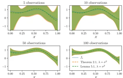
The following experiments compare the concentration result given by Theorem 1 with the kernel concentration bounds from Wang and de Freitas (2014) reported by Lemma 3. The true noiseσ = 0.1 is assumed to be known and all observations are uniformly sampled from X. In both cases, we use a fixed confidence levelδ= 0.1. Figure 2 shows that forλ=σ2, the
2. Ifx∈R, thei-th feature of a Gaussian kernelϕ(x) =e
−x2
2ρ2 xi−1
0.00 0.25 0.50 0.75 1.00 X
0.0 0.5 1.0
Figure 1: Test function f? used in the following numerical experiments.
0.00 0.25 0.50 0.75 1.00 X
−1 0 1
5 observations
0.00 0.25 0.50 0.75 1.00 X
−1 0 1
10 observations
0.00 0.25 0.50 0.75 1.00 X
−1 0 1
50 observations
0.00 0.25 0.50 0.75 1.00 X
−1 0 1
100 observations
f?
Theorem 2.1,λ=σ2
Lemma 5.1,λ=σ2
Figure 2: Confidence interval of Theorem 1 and Lemma 3 (Wang and de Freitas, 2014).
result given by Theorem 1 recovers the confidence envelope of Wang and de Freitas (2014). Note however that the confidence bound that we plot for Theorem 1 are valid uniformly
over all time steps, while the one derived from Wang and de Freitas (2014) is only valid separately for each time. Further, Theorem 1 generalizes the latter result to the case where
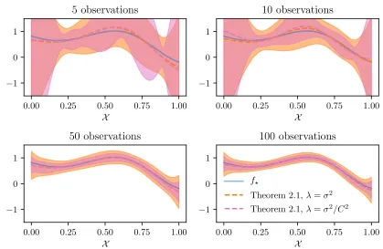
λ 6= σ2. For illustration, Figure 3 illustrates the confidence envelopes in the special case whereλ=σ2/C2, which also shows the potential benefit of such a tuning.
6.2 Empirical variance estimate
0.00 0.25 0.50 0.75 1.00 X
−1 0 1
5 observations
0.00 0.25 0.50 0.75 1.00 X
−1 0 1
10 observations
0.00 0.25 0.50 0.75 1.00 X
−1 0 1
50 observations
0.00 0.25 0.50 0.75 1.00 X
−1 0 1
100 observations
f?
Theorem 2.1,λ=σ2
Theorem 2.1,λ=σ2/C2
Figure 3: Confidence interval of Theorem 1 for different λ.
0 100 200 300 400 500
t 10−1
100 σ+
,t
σ+= 1
σ+= 5
(a)
0 100 200 300 400 500
t 10−1
100 σ+
,t
σ+= 1
σ+= 5
(b)
Figure 4: Noise estimate from Theorem 3 withσ+for a) fixedλ=σ2+/C2; b)λ=σ+2,t−1/C2. Dotted line indicatesσ.
and δ = 0.1. All observations are uniformly sampled from X. Section 3 suggests that
λ = σ2
+,t−1/C2 should provide tighter bounds than a fixed λ = σ+2/C2. Figure 4 shows that this is indeed the case especially for large values of t. We also see that the adaptive update of λconverges to the same value, whatever the initial boundσ+. This is especially interesting whenσ+ is a loose initial upper bound onσ.
0 100 200 300 400 500 t
10−1
100 σ+
,t
Unknownσ+
σ+= 1.0
(a)
0 100 200 300 400 500
t 10−2
10−1
100
σ+
,t
σ+= 1.0
σ+= 0.5
σ+= 0.1
(b)
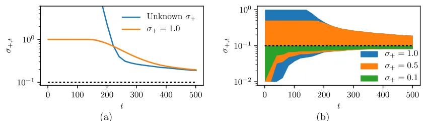
Figure 5: Variance estimate a) from Theorem 3, with and without σ+; b) as minimum of the bounds and σ+, for different upper-bounds. Dotted line indicatesσ.
setσ+,t(λ, λ−) and the maximum forσ−,t(λ). Figure 5b shows the resulting noise estimate
envelopes for differentσ+ values (recall thatσ = 0.1).
6.3 Kernel concentration bound with adaptive regularization
We now combine the previous experiments and use the estimated noise in order to tune the regularization. Recall that we consider σ−,0 = σ−, σ+,0 =σ+, and λ0 = σ+2/C2. On each time t >1, we estimate the noise lower-bound σ−,t = max{σ−,t(λt−1), σ−,t−1} using Theorem 3 and set λ− = σ−2,t/C2. We then compute the upper-bound noise estimate
σ+,t = min{σ+,t(λt−1, λ−), σ+,t−1} using Theorem 3 and set λt = σ2+,t/C2. We are now
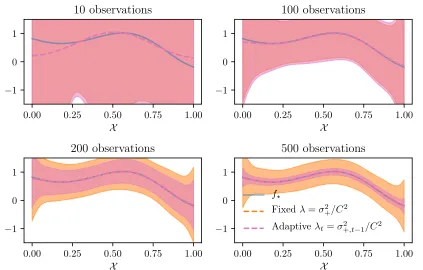
ready to compute the confidence interval given by Corollary 1. Note that δ = 0.1 is used everywhere and all observations are uniformely sampled from X. Figure 6 illustrates the resulting confidence envelope of this fully empirical model for noise upper-bound σ+ = 1 (recall that the noise satisfiesσ= 0.1) plotted against the confidence envelope obtained with Theorem 1 with fixedλ=σ2
+/C2. We observe the improvement of the confidence intervals with the number of observations. Recall that this setting is especially challenging since the variance is unknown, the regularization parameter is tuned online, and the confidence bounds are valid uniformly over all time steps.
6.4 Kernelized bandits optimization
In this section, we now evaluate the potential of kernelized bandits algorithms with variance estimate. We consider Xas the linearly discretized space X = [0,1] into 100 arms. Recall that the goal is to minimize the cumulative regret (Equation 4) and that we are optimizing the function shown by Figure 1 with σ = 0.1. We evaluate Kernel UCB (Equation 5) and Kernel TS (Algorithm 1 withvt=Bλt,t−1(δ)/σ+,t−1) with three different configurations:
a) the oracle, that is with fixed λt=σ2/C2, assuming knowledge ofσ;
b) the fixed λt=σ2+/C2, that is the best one can do without prior knowledge of σ2; c) the adaptative regularization tuned with Corollary 1.
0.00 0.25 0.50 0.75 1.00 X
−1 0 1
10 observations
0.00 0.25 0.50 0.75 1.00 X
−1 0 1
100 observations
0.00 0.25 0.50 0.75 1.00 X
−1 0 1
200 observations
0.00 0.25 0.50 0.75 1.00 X
−1 0 1
500 observations
f?
Fixedλ=σ2 +/C2
Adaptive λt=σ+2,t−1/C2
Figure 6: Confidence interval using fixed (Theorem 1) and adaptive (Corollary 1) regular-ization, forσ+= 1 andδ = 0.1.
0 100 200 300 400 500 Episodes (t)
0 25 50 75 100 125 150
Cum
ulativ
e
regret
Kernel UCB oracle Kernel UCB fixed Kernel UCB adaptative
(a)
0 100 200 300 400 500 Episodes (t)
0 25 50 75 100 125 150
Cum
ulativ
e
regret
Kernel TS oracle Kernel TS fixed Kernel TS adaptative
(b)
Figure 7: Averaged cumulative regret along episodes for a) Kernel UCB and b) Kernel TS.
0 100 200 300 400 500 Episodes (t)
0 10 20 30 40
Cum
ulativ
e
regret
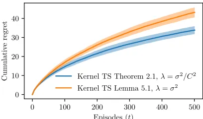
Kernel TS Theorem 2.1,λ=σ2/C2 Kernel TS Lemma 5.1,λ=σ2
Figure 8: Averaged cumulative regret and one standard deviation along episodes for Kernel TS oracle with Theorem 1 and Lemma 3 (Wang and de Freitas, 2014).
In order to evaluate the benefit of the concentration bound provided by Theorem 1, we compare the Kernel TS (Algorithm 1) oracle using vt =Bλ,t−1/σ and λ = σ2/C2, where
Bλ,t−1 is given by Theorem 1, against vt =`t(δ) where `t(δ) is given by Lemma 3 (Wang
and de Freitas, 2014) with δ= 0.1. Figure 8 shows that the concentration bound given by Theorem 1 improves the performance of Kernel TS compared with existing concentration results (Wang and de Freitas, 2014). It highlights the relevance of expliciting the regular-ization parameter, which allows us to take advantage of regularregular-ization rates that may be better adapted.
7. Conclusion
This work addresses two problems: the online tuning of the regularization parameter in streaming kernel regression and the online estimation of the noise variance. To this extent, we introduce novel concentration bounds on the posterior mean estimate in streaming kernel regression with fixed and explicit regularization (Theorem 1), which we then extend to the setting where the regularization parameter is tuned (Theorem 2). We further introduce upper- and lower-bound estimates of the noise variance (Theorem 3). Putting these tools together, we show how the estimate of the noise variance can be used to tune the kernel regularization in an online fashion (Corollary 1) while retaining theoretical guarantees. We also show how to use the proposed results in order to derive kernelized variations of the most common bandits algorithms UCB and Thompson sampling, for which regret bounds are also provided (Theorems 4 and 5).
Future work includes a natural extension of these techniques to obtain an empirical estimate of the kernel length scales. This information is often assumed to be known, while in practice it is often not available. Although some preliminary work has been done in that direction (Wang and de Freitas, 2014), designing theoretically motivated algorithms addressing these concerns would help to fill an important gap between theory and practice. On a different matter, the current work gives the basis for performing Thompson sampling in RKHS, and could be extended to the contextual setting in a near future, as was done with CGP-UCB (Krause and Ong, 2011; Valko et al., 2013).
Acknowledgments
This work was supported through funding from the Natural Sciences and Engineering Re-search Council of Canada (NSERC, Canada), the REPARTI strategic network (FRQ-NT, Qu´ebec), MITACS, and E Machine Learning Inc. O.-A. M. acknowledges the support of the French Agence Nationale de la Recherche (ANR), under grant ANR-16-CE40-0002 (project BADASS), Inria Lille – Nord europe, CPER Nord-Pas de Calais/FEDER DATA Advanced data science and technologies 2015-2020, and the French Ministry of Higher Education and Research.
Appendix A. Laplace method for tuned kernel regression
In this section, we want to control the term|fλ,t(x)−f?(x)|simultaneously over all t6T.
To this end, we resort to a version of the Laplace method carefully extended to the RKHS setting.
Before proceeding, we note that since k : X × X → R is a kernel function (that is continuous, symmetric positive definite) on a compact setX equipped with a positive finite Borel measure µ, then there is an at most countable sequence (σi, ψi)i∈N? where σi > 0, limi→∞σi = 0 and {ψi}form an orthonormal basis of L2,µ(X), such that
k(x, y) =
∞
X
j=1
σjψj(x)ψj(y0) and kf?k2K= ∞
X
j=1
hf, ψji2L2,µ
σj
Let ϕi = √σiψi. Note that kϕikL2 = √σ
i, kϕikK = 1. Further, if f = Piθiϕi, then
kf?k2K =
P
iθi2 and kf?k2L2 = Piθi2σi. In particular f belongs to the RKHS if and only
if P
iθi2 < ∞. For ϕ(x) = (ϕ1(x), . . .) and θ = (θ1, . . .), we now denote θ>ϕ(x) for
P
i∈Nθiϕi(x), by analogy with the finite dimensional case. Note that k(x, y) =ϕ(x)>ϕ(y).
In the sequel, the following Martingale control will be a key component of the analysis.
Lemma 4 (Hilbert Martingale Control) Assume that the noise sequence {ξt}∞t=0 is
conditionally σ2-sub-Gaussian
∀t∈N,∀γ ∈R, lnE[exp(γξt)|Ht−1]6
Let τ be a stopping time with respect to the filtration {Ht}∞t=0 generated by the variables {xt, ξt}∞t=0. For any q= (q1, q2, . . .) such that q>ϕi(x) =Pi∈Nqiϕ(x)<∞, and
determin-istic positive λ, let us denote
Mm,λq = exp
m
X
t=1
q>ϕ(xt)
√
λ ξt−
σ2 2
m
X
t=1
(q>ϕ(xt))2
λ
Then, for all suchq the quantity Mτ,λq is well defined and satisfies
lnE[Mτ,λq ]60.
Proof The only difficulty in the proof is to handle the stopping time. Indeed, for all
m ∈ N, thanks to the conditional R-sub-Gaussian property, it is immediate to show that {Mm,λq }∞m=0 is a non-negative super-martingale and actually satisfies lnE[Mm,λq ]60.
By the convergence theorem for nonnegative super-martingales, M∞q = limm→∞Mm,λq
is almost surely well-defined, and thus Mτ,λq is well-defined (whetherτ <∞or not) as well. In order to show that lnE[Mτ,λq ]60, we introduce a stopped versionQmq =Mminq {τ,m},λ of
{Mm,λq }m. Now E[Mτ,λq ] =E[lim infm→∞Qqm]6lim infm→∞E[Qqm]61 by Fatou’s lemma,
which concludes the proof. We refer to (Abbasi-Yadkori et al., 2011) for further details.
We are now ready to prove the following result.
Proof of Theorem 2 (Streaming Kernel Least-Squares) We make use of the features in an explicit way. Let λ = λt+1. For f? ∈ K, we denote θ? its corresponding parameter
sequence. We letΦt= (ϕ(xt0))t06tbe at× ∞matrix built from the features and introduce the bi-infinite matrix Vλ,t = I + λ1Φ>t Φt as well as the noise vector Et = (ξ1, . . . , ξt). In
order to control the term |fλ,t−f?(x)|, we first decompose the estimation term. Indeed,
using the feature map, it holds that
fλ,t(x) = kt(x)>(Kt+λIt)−1Yt
= ϕ(x)>Φ>t(ΦtΦ>t +λIt)−1Yt
= ϕ(x)>Φ>t
It
λ −
1
λΦt λI+Φ
> t Φt
−1
Φ>t
Yt
= ϕ(x)>(Φ>t Φt+λI)−1Φ>t(Φtθ?+Et)
where in the third line, we used the Shermann-Morrison formula. From this, simple algebra yields
fλ,t(x)−f?(x) =
1
λϕ(x)
>
Vλ,t−1 Φ>tEt−λθ?
.
We then obtain, from a simple H¨older inequality using the appropriate matrix norm, the following decomposition, that is valid provided that all terms involved are finite.
|fλ,t(x)−f(x)|6
1 √
λkϕ(x)kVλ,t−1
1 √
λkΦ
> t EtkV−1
λ,t +
√
λkθ?kVλ,t−1
Now, we note that a simple application of the Shermann-Morrison formula yields
kϕ(x)k2V−1 λ,t
=kt(x, x).
On the other hand, the last term of the bound is controlled as kθ?k
Vλ,t−1 6kθ?k. Thus,
|fλ,t(x)−f(x)|6
kλ1/,t2(x, x)
p λt+1
1
p λt+1
kΦ>t EtkV−1 λt+1,t
+pλt+1kθ?k2
.
In order to control the remaining term, √1
λt+1k
Φ>t EtkV−1 λt+1,t
, for all t, we now want to
apply Lemma 4. However, the lemma does not apply since λt+1 is Ht-measurable. Thus,
before proceeding, we upper-bound it by the similar expression involvingλ?:
1
λkΦ
> t Etk2V−1
λ,t
= Et>Φ
> t
λ (I+
1
λΦ
> t Φt)−1
Φt
Et
= Et>Φ>t (λI+Φ>t Φt)−1ΦtEt
6 Et>Φ>t (λ?I+Φ>t Φt)−1ΦtEt,
where in the last line, we use the fact that the functionf :λ→u>(λI+A)−1u, foru=Φ
tEt
and A = Φ>t Φt is non increasing (see Lemma 5 below). Thus, √1 λt+1k
Φ>tEtkV−1 λt+1,t 6 1
√ λ?kΦ
>
λ?,tEtkVλ?,t−1 . Next, we introduce a random stopping timeτ, to be defined later and apply Lemma 4.
More precisely, let Q ∼ N(0, I) be an infinite Gaussian random sequence which is independent of all other random variables. We denote Q>ϕ(x) = P
i∈NQiϕi(x). For all
x, k(x, x) = P
i∈Nϕ 2
i(x) < ∞ and thus V(Q>ϕ(x)) < ∞. We define Mm,λ? = E[M Q m,λ?]. Clearly, we still haveE[Mλ?,τ] =E[E[M
Q
m,λ?]|Q]61. SinceVλ?,τ =I+ 1
λ?Φ
>
τΦτ, elementary
algebra gives
det(Vλ?,τ) = det(Vλ?,τ−1+ 1
λ?
ϕ(xτ)ϕ(xτ)>) = det(Vλ?,τ−1)(1 + 1
λ?k
ϕ(xτ)k2V−1 λ?,τ−1
)
= det(Vλ?,0) τ
Y
t0=1
1 + 1
λ?k
ϕ(xt0)k2 V−1
λ?,t0−1
,
where we used the fact that the eigenvalues of a matrix of the form I +xx> are all ones except for the eigenvalue 1 +kxk2 corresponding tox. Then, note that det(V
λ?,0) = 1 and thus
ln(det(Vλ?,τ)) = τ
X
t0=1
ln(1 + 1
λ?k
ϕ(xt0)k2 Vλ?,t0−−1 1)
= 1 2
τ
X
t0=1 ln
1 + 1
λ?
kλ?,t0−1(xt0, xt0)
.
using the d first dimension of the sequence for each d. We note Qd, Mλ?,τ,Φτ,d and Vτ,d the restriction of the corresponding quantities to the components {1, . . . , d}. Thus Qd is
GaussianN(0, Id). Following the steps from Abbasi-Yadkori et al. (2011), we obtain that
Mm,d,λ? =
1 det(Vλ?,m,d)1/2
exp
1 2σ2λ
?k
Φ>m,dEmk2V−1 λ?,m,d
.
Note also that E[Mτ,d,λ?]6 1 for all d∈N. Thus, we obtain by an application of Fatou’s lemma that
P
lim
d→∞
kΦ>τ,dEτk2V−1 λ?,τ,d
2σ2λ
?log
det(Vλ?,τ,d)1/2/δ
>1
6 E
lim
d→∞
δexp
1 2λ?σ2kΦ
>
τ,dEτk2V−1 τ,d
det(Vλ?,τ,d)1/2
6 δ lim
d→∞E[Mτ,d,λ?]6δ .
We conclude by definingτ following Abbasi-Yadkori et al. (2011), by
τ(ω) = min
t>0;ω∈Ω s.t. kΦ>tEtk2V−1 λ?,t
>2σ2λ?log
det(Vλ?,t) 1/2/δ
.
Then τ is a random stopping time and
P
∃t,kΦ>tEtk2V−1 λ?,t
>2σ2λ
?log
det(Vλ?,t) 1/2/δ
=P(τ <∞)6δ.
Finally, combining this result with the previous remarks we obtain that with probability higher than 1−δ, uniformly over x∈ X and t6T, it holds that
|fλ,t−f?(x)|6
kλ1/,t2(x, x)
p λt+1
s
2σ2ln
det(I+ 1
λ?Φ
> tΦt)1/2
δ
+pλt+1kf?kK
.
Lemma 5 (Technical lemma) The function f :λ7→u>(λI+A)−1u, whereA is a
semi-definite positive matrix andu is any vector, is non-decreasing onλ∈R+. Proof Indeed, let h >0. By the Sherman-Morrison formula, we obtain
f(λ+h) =f(λ)−hu>(λI+A)−1(I+h(λI+A)−1)−1(λI+A)−1u .
Thus, sinceλI+A is also semi-definite positive, we have
lim
h→0
f(λ+h)−f(λ)
h =−u
>(λI+A)−1(λI+A)−1u
Appendix B. Variance estimation
In this section, we give the proof of Theorem 3. To this end, we proceed in two steps. First, we provide an upper bound and lower bound on the variance estimate in the next theorem. Then, we use these bounds in order to derive the final statement.
Theorem 6 (Regularized variance estimate) Under the second-order sub-Gaussian pre-dictable assumption, for any random stopping time τ for the filtration of the past, with probability higher than 1−3δ, it holds
q
b σ2
k,λ,τ 6 σ
1 +
r
2Cτ(δ)
τ
+kf?kK
r λ τ
s
1− 1
maxt6τ(1 +kλ,t−1(xt, xt))
q
b σ2
k,λ,τ > σ
1−
r Cτ(δ)
τ −
r
Cτ(δ) + 2Dλ?,τ(δ)
τ
−
s
2σλ1/2kf?kKp
Dλ?,τ(δ)
τ .
where we introduced for convenience the constantsCτ(δ) = ln(e/δ)
1+ln(π2ln(τ)/6)/ln(1/δ)
and Dλ?,τ(δ) = 2 ln(1/δ) +
Pτ
t=1ln(1+ 1
λ?kλ?,t−1(xt, xt)).
Proof We use the feature maps and start with the following decomposition
τbσ
2
k,λ,τ = τ
X
t=1
(yt−fλ,τ(xt))2 = τ
X
t=1
(yt− hθλ,τ, ϕ(xt)i)2
= (θ?−θλ,τ)>Gτ(θ?−θλ,τ) +kEτk2+ 2(θ?−θλ,τ)>Φ>τEτ. (6)
whereθ?−θ
λ,τ = (I−G−λ,τ1Gτ)θ?−G−λ,τ1Φτ>Eτ with Gλ,τ =λI+Gτ and Gτ = Φ>τΦτ.
On the one hand, we can control the first term in (6) via
(θ?−θλ,τ)>Gτ(θ?−θλ,τ)
= [(I−G−λ,τ1Gτ)θ?−G−λ,τ1Φ>τEτ]>Gτ[(I−G−λ,τ1Gτ)θ?−G−λ,τ1Φ>τEτ]
= [λθ?−Φ>τEτ]>G−λ,τ1GτG−λ,τ1[λθ?−Φ>τEτ]
= [λθ?−Φ>τEτ]>[Gλ,τ−1 −λG−λ,τ2][λθ?−Φ>τEτ]
= kΦ>τEτk2G−1 λ,τ −
λkΦ>τEτk2G−2 λ,τ
+λ2kθ?k2
G−λ,τ1 −λ
3kθ?k2
G−λ,τ2
−2λθ?>[G−λ,τ1 −λG−λ,τ2]Φ>τEτ
where we used the fact thatI−G−λ,τ1Gτ =λG−λ,τ1 and then thatG −1
λ,τGτG−λ,τ1 =G −1
λ,τ−λG −2
λ,τ.
Likewise, we control the third term in (6) via
2(θ?−θλ,τ)>Φ>τEτ = 2[(I−G−λ,τ1Gτ)θ?−G−λ,τ1Φ >
τEτ]>Φ>τEτ
= 2[λθ?−Φ>τEτ]>G−λ,τ1Φ>τEτ
= 2λθ?>G−λ,τ1Φ>τEτ −2kΦ>τEτk2G−1 λ,τ
Combining these two bounds, we have
τ
X
t=1
(yt− hθλ,τ, ϕ(xt)i)2
= kEτk2− kΦ>τEτk2G−1 λ,τ −
λkΦ>τEτk2G−2 λ,τ
+λ2kθ?k2G−1 λ,τ −
λ3kθ?k2G−2 λ,τ
+ 2λ2θ?>G−λ,τ2Φ>τEτ
6 kEτk2+
λ2
λmin(Gλ,τ)
kθ?k2 2
1− λ
λmax(Gλ,τ)
+ 2 λ 2
λmin3/2(G λ,τ)
kθ?k2kΦ>τEτkG−1 λ,τ
> kEτk2+
λ2
λmax(Gλ,τ)k
θ?k2 2
1− λ
λmin(Gλ,τ)
−2 λ 2
λmin3/2(G λ,τ)
kθ?k2kΦ>τEτkG−1 λ,τ
−kΦ>τEτk2G−1 λ,τ
1 + λ
λmin(Gλ,τ)
.
Now, from Lemma 6, it holds on an event Ω1 of probability higher than 1−δ,
06kΦ>τEτk2G−1 λ,τ
= 1
λkΦ
>
τEτk2V−1 λ,τ 6
1
λ?k
Φ>τEτk2V−1 λ?,τ 6
σ2Dλ?,τ(δ).
On the other hand, we control the second term kEτk2 by Lemma 6 below, and obtain
that with probability higher than 1−2δ,
kEτk2 6 τ σ2+ 2σ2
p
2τ Cτ(δ) + 2σ2Cτ(δ)
kEτk2 > τ σ2−2σ2
p
τ Cτ(δ),
whereCτ(δ) = ln(e/δ)(1 +cτ/ln(1/δ)).
Thus, combining these two results with a union bound, we deduce that with probability higher than 1−3δ it holds that
b
σ2λ,τ 6 σ2+ 2σ2 r
2Cτ(δ)
τ +
2σ2C
τ(δ)
τ
+ λ
2
τ λmin(Gλ,τ)kθ
?
k22
1− λ
λmax(Gλ,τ)
−2 σλ 2
τ λmin3/2(G λ,τ)
kθ?k2
q
Dλ?,τ(δ)
b σ2
λ,τ > σ2−2σ2
r Cτ(δ)
τ +
λ2
τ λmax(Gλ,τ)k
θ?k2 2
1− λ
λmin(Gλ,τ)
−2 λ 2σ
τ λmin3/2(G λ,τ)
kθ?k2
q
Dλ?,τ(δ)−
σ2D
λ?,τ(δ)
τ
1 + λ
λmin(Gλ,τ)
We can now derive a bound onqbσ2
λ,τ. Indeed,
b σλ,τ2 6
σ+
r
2σ2C
τ(δ)
τ 2
+ λ
2
τ λmin(Gλ,τ)kθ
?
k22
1− λ
λmax(Gλ,τ)
b σ2 λ,τ > σ− r σ2C
τ(δ)
τ 2 −σ 2 τ
Cτ(δ) +Dλ?,τ(δ)
1 + λ
λmin(Gλ,τ)
− 2λ 2σ
τ λmin3/2(G λ,τ)
kθ?k2
q
Dλ?,τ(δ).
Thus, using the inequality √a+b6√a+√b, on both inequalities, we get
q
b σ2
λ,τ 6 σ+σ
r
2Cτ(δ)
τ +
λkθ?k
2
q
τ λmin(Gλ,τ)
s
1− λ
λmax(Gλ,τ)
q
b σ2
λ,τ > σ−σ
r Cτ(δ)
τ −σ
v u u
tCτ(δ) +Dλ?,τ(δ)
1+ λ λmin(Gλ,τ)
τ −λ v u u t
2σkθ?k
2
p
Dλ?,τ(δ)
τ λmin3/2(G λ,τ)
.
Corollary 1 (Extension of Corollary 3.13 in Maillard (2016)) With probability higher than 1−3δ0, it holds simultaneously over all t>0,
σ6 1
α2
s√
λkf?kK
p Dt,λ?(δ
0)
2t +
s√
λkf?kK
p Dλ?,t(δ
0)
2t +bσλ,tα !2
σ>
b
σλ,t− kf?kK
s λ
t
1− 1
maxt06t(1 +kλ,t0−1(xt0, xt0))
1 +
r
2Ct(δ0)
t
−1 ,
where α = max
1−
q
Ct(δ0)
t −
q
Ct(δ0)+2Dλ?,t(δ0)
t ,0
. Further, if an upper bound σ+ >σ
is known, one can derive the following inequalities that hold with probability higher than
1−3δ0,
σ6bσλ,t+σ
+
r Ct(δ0)
t +
r
Ct(δ0) + 2Dλ?,t(δ
0)
t
+
s
2σ+λ1/2kf
?kK
p
Dt,λ?(δ0)
t
σ>bσλ,t−σ
+
r
2Ct(δ0)
t − kf?kK s
λ t
1− 1
maxt06t(1 +kλ,t0−1(xt0, xt0))
Proof Using Theorem 6, it holds with high probability that b σλ,τ |{z} A >σ 1− r Cτ(δ0)
τ −
r
Cτ(δ0) + 2Dλ?,τ(δ0)
τ
| {z }
C
−√σ s
2√λkf?kKpDλ?,τ(δ
0)
τ
| {z }
B
.
The inequality rewrites A >σC−√σB. Now, let y2 =σ. If C >0, the inequality holds provided that y > 0 and A+yB −Cy2 > 0, that is when 0 6 y 6 B+√B2+4AC
2C . We
conclude by choosing the stopping time τ corresponding to the probability of bad events, as in the proof of Theorem 2, then by remarking thatt7→Ct(δ0) is an increasing function.
Lemma 6 (Lemma 5.10 from Maillard (2016)) Assume thatTn is a random stopping time that satisfies Tn6n almost surely, then
P 1 Tn Tn X i=1
ξi2 >σ2+ 2σ2 s
2 ln(e/δ)
Tn
+ 2σ2ln(e/δ) Tn
6
dln(n) ln(e/δ)eδ ,
P 1 Tn Tn X i=1
ξi26σ2−2σ2 s
ln(e/δ)
Tn
6dln(n) ln(e/δ)eδ .
Further, for a random stopping time T, and if we introduce cT = ln(π2ln2(T)/6), then
P 1 T T X i=1
ξi2>σ2+2σ2 r
2 ln(e/δ)(1 +cT/ln(1/δ))
T + 2σ
2ln(e/δ)(1 +cT/ln(1/δ))
T
6δ ,
P 1 T T X i=1 ξ2
i 6σ2−2σ2
r
ln(e/δ)(1 +cT/ln(1/δ))
T
6δ .
Appendix C. Application to stochastic multi-armed bandits
Proof of Lemma 1 Using the facts that min{r, α}6(α/ln(1+α)) ln(1+r) and minλ∈λλ>
σ2/C2:
T
X
t=1
s2
λ,t−1(xt) =σ2 T
X
t=1 1
λt
kλt,t−1(xt, xt)
6σ2
T
X
t=1
C2
σ2kσ2/C2,t−1(xt, xt) =σ2
T
X
t=1
minnC 2
σ2kσ2/C2,t−1(xt, xt),
C2
σ2
o
6 2C
2
In particular, we obtain by a Cauchy-Schwarz inequality,
T
X
t=1
s
kλt,t−1(xt, xt)
λt 6
s
T 2C2/σ2
ln(1 +C2/σ2)γT(σ2/C2).
Proof of Lemma 2 We want to control the quantity Bλt,t(δ). First of all, recall from Equation 3 that
Bλt,t(δ) =
p
λtC+σ+,t
p
2 ln(1/δ) + 2γt(λ−)
6σ++σ+
q
2 ln(1/δ) + 2γt(σ2t,−/C2),
where we use the facts that λt 6σ+2/C2 and λ− >σ2t,−/C2. Then, using that σt,2− >σ−,
thatγt(·) is non-increasing and non-decreasing with t, it comes
Bλt,t(δ)6σ++σ+
q
2 ln(1/δ) + 2γT(σ−2/C2).
Alternatively one may use Theorem 6 in order to control the random variables σt,+ and σt,− in a tighter way. For instance, by Theorem 6, we easily obtain that with high
probability, for all t,
σ >σt,− > σ−
σ
√
t
(√2 + 1)p
Ct(δ)−
p
Ct(δ) + 2Dλ?,t(δ)
1 +p
2Ct(δ)/t
−
q
2σλ1/2kf?k K
p
Dλ?,t(δ) +C
√
λq1− 1
maxt6t(1+kλ,t−1(xt,xt))
√
t(1 +p
2Ct(δ)/t)
,
that is the estimate satisfies σ > σt,− > σ −O(1/
√
t). This in turns implies that
γt(σ2−,t/C2) 6 γt(σ2/C2) +O(1/
√
t). Likewise, it can be shown that σ 6 σt,+ 6 σ+
O(1/√t),which yields
Bλt,t(δ)6σ
1 +
q
2 ln(1/δ) + 2γT(σ2−/C2)
+o(1).
Proof of Theorem 4 (UCB algorithm for kernel bandits) Letrt denote the
instan-taneous regret at timetandf+(x
t) denote the optimistic value at the chosen pointxt, built
from the confidence set used by the UCB algorithm. The following holds with probability higher than 1−4δ for each time-step t
rt(λt) = f?(x?)−f?(xt)6ft+−1(xt)−f?(xt)
6 |ft+−1(xt)−fλt,t−1(xt)|+|fλt,t−1(xt)−f?(xt)|
6 2
s
kλt,t−1(xt, xt)
λt
Thus, we deduce that with probability higher than 1−4δ:
RT =
T
X
t=1
rt(λ)62 T
X
t=1
s
kλt,t−1(xt, xt)
λt
Bλt,t−1(δ).
We then use Lemma 2 in order to control the term Bλt,t−1(δ), and Lemma 1 in order to control the sum of kλt,t−1(xt,xt)
λt . This yields the following bound on the regret:
RT 6 2σ+
1 +
q
2 ln(1/δ) + 2γT(σ−2/C2)
s
T 2C
2/σ2
ln(1 +C2/σ2)γT(σ2/C2).
Proof of Theorem 5 (TS algorithm for kernel bandits) We closely follow the proof technique of Agrawal and Goyal (2013), while clarifying and simplifying some steps. The general idea is to split the arms into two groups: saturated arms andunsaturated arms. The former designates arms where samples ˜ft have low probability of dominatingf?(x?) while
the latter designates the other case. This is related to the optimism (Abeille and Lazaric, 2017), that is the possibility of sampling a value that is higher than the optimum. Let Ebt
and ˜Et be the events thatfbt and ˜ft are concentrated around their respective means. More
precisely, for a given confidence level δ, we introduce
b
Et,δ = {∀x∈ X,|f?(x)−fλt,t−1(x)|6Cbt,δ(x)} ˜
Et,δ = {∀x∈ X,|fλt,t−1(x)−f˜t(x)|6C˜t,δ(x)}, for some quantities Cbt,δ(x),C˜t,δ(x) to be defined.
Controlling the event Ebt,δ Choosing the confidence bound to be
b
Ct,δ(x) =
s
kλt,t−1(x, x)
λt
Bλt,t−1(δ/4),
then the event Ebt,δ is controlled as P
∀t>0, Ebt,δ
>1−δ.
Controlling the event E˜t,δ On the other hand, since ˜ft(x)|Ht−1 = N(fλt,t−1(x),Vt) where we introduced the notation Vt = vt2
σ2 +,t−1
λt (kλt,t−1(x, x
0)) x,x0∈
X, then we have by a simple union bound overx∈X,
P( ˜Et,δc |Ht−1)6
X
x∈X
1 √
πzx
e−zx2/2
provided that zx =
˜
Ct,δ(x) vt
r σ2+,t−1
λt kλt,t−1(x,x)
> 1 for all x ∈ X. This motivates the following
definition,
˜
Ct,δ(x) =ct,δvt
s σ2
+,t−1
λt
for a well-chosen sequence (ct,δ)t. The choicect,δ= max{
p
2 ln(t(t+ 1)|X|/√πδ),1}ensures that
P(∃t>0 ˜Et,δc |Ht−1) 6
X
t>0 |X| √
πct,δ
e−c2t,δ/2 =X t>0
δ ct,δt(t+ 1)
6 X
t>0
δ
t(t+ 1) =δ,
from which we obtain P
∀t>0, E˜t,δ
>1−δ.
Summary By definition of the events, under Ebt,δ and ˜Et,δ, it thus holds that
∀x∈ X,
f?(x)−
˜
ft(x)
6
f?(x)−fλt,t−1(x)
+
fλt,t−1(x)−
˜
ft(x)
6 Cbt,δ(x) + ˜Ct,δ(x)
=
s
kλt,t−1(x, x)
λt
Bλt,t−1(δ/4) +ct,δvtσ+,t−1
= sλ,t−1(x)
Bλt,t−1(δ/4)
σ +ct,δvt
σ+,t−1
σ
| {z }
gt(δ)
.
Saturated arms It is now convenient to introduce the set of saturated times a time t
St,δ=
x∈X:f?(x?)−f?(x)> sλ,t−1(x)gt(δ)
together with xS,t= argmin x /∈St,δ
sλ,t−1(x).
We remark that by construction ? /∈ St,δ for allt. Now, by the strategy of the Kernel TS
algorithm,xt= argmaxx∈Xf˜t(x). Thus, we deduce that on the eventEbt,δ∩E˜t,δ
f?(x?)−f?(xt) = f?(x?)−f?(xS,t) +f?(xS,t)−f?(xt)
6 sλ,t−1(xS,t)gt(δ) +
f?(xS,t)−f˜t(xS,t)
+f˜t(xS,t)−f˜t(xt)
| {z }
60
+f˜t(xt)−f?(xt)
6 2sλ,t−1(xS,t)gt(δ) +sλ,t−1(xt)gt(δ).
Also, f?(x?)−f?(xt) 6R, where R = maxx∈Xf?(x?)−f?(x) <∞. We then remark that by definition ofxS,t, we have
E[sλ,t−1(xt)|Ht−1] > E[sλ,t−1(xt)I{xt∈ S/ t,δ}|Ht−1]
> E[sλ,t−1(xS,t)I{xt∈ S/ t,δ}|Ht−1] = sλ,t−1(xS,t)P
xt∈ S/ t,δ
Ht
−1
Likewise,
min{sλ,t−1(xS,t)gt(δ), R}6 E
[min{2sλ,t−1(xt)gt(δ), R}|Ht−1] P
xt∈ S/ t,δ
Ht −1 .
Since on the other hand, (f?(x?)−f?(xt))I{xt ∈ S/ t,δ} 6 sλ,t−1(xt)gt(δ)I{xt ∈ S/ t,δ}, we
deduce that on the eventEbt,δ∩E˜t,δ we have
f?(x?)−f?(xt) 6 min
2sλ,t−1(xS,t)gt(δ) +sλ,t−1(xt)gt(δ), R
I{xt∈ St,δ}
+sλ,t−1(xt)gt(δ)I{xt6∈ St,δ}
6 minn2sλ,t−1(xS,t)gt(δ), R
o
I{xt∈ St,δ}+sλ,t−1(xt)gt(δ)
6 E[min{2sλ,t−1(xt)gt(δ), R}|Ht−1]
P
xt∈ S/ t,δ
Ht−1
I{xt∈ St,δ}+sλ,t−1(xt)gt(δ).
Lower bounding the denominator At this point, we note that on the eventEbt,δ∩E˜t,δ,
for all x∈ St,δ,
˜
ft(x)6f?(x) +sλ,t−1(x)gt(δ)6f?(x?),
while on the other hand we have the inclusion {∀x∈ St,δ, f˜t(x?)>f˜t(x)} ⊂ {xt6∈ St,δ}.
Thus, combining these two properties, we deduce that
{xt∈ St,δ} ∩Ebt,δ∩E˜t,δ
⊂ n∃x∈ St,δ,f˜t(x?)6f˜t(x)
o
∩n∀x∈ St,δ,f˜t(x)6f?(x?)
o
⊂ nf˜t(x?)6f?(x?)
o .
Further, using that ˜ft(x)|Ht−1 =N(fλt,t−1(x),Vt) yields
{xt∈ St,δ} ∩Ebt,δ∩E˜t,δ
⊂ nf˜t(x?)−fλt,t−1(x?)6f?(x?)−fλt,t−1(x?)
o
∩Ebt,δ∩E˜t,δ
⊂ nf˜t(x?)−fλt,t−1(x?)6Cbt,δ(x?) o
⊂n
f˜t(x?)−fλt,t−1(x?)
6Cbt,δ(x?) o
,
from which we obtain
n
f˜t(x?)−fλt,t−1(x?)
>Cbt,δ(x?) o
∩Ebt,δ ⊂ {xt6∈ St,δ} ∪E˜t,δc .
Thus, we have proved that
P
xt∈ S/ t,δ
Ht −1 > P
f˜t(x?)−fλt,t−1(x?)
>Cbt,δ(x?),Ebt,δ Ht −1 −P ˜ Ec t,δ Ht−1
= P
f˜t(x?)−fλt,t−1(x?)
>Cbt,δ(x?) Ht −1
I{Ebt,δ} −P
˜
Et,δc Ht−1