Invariant Models for Causal Transfer Learning

Invariant Models for Causal Transfer Learning

Mateo Rojas-Carulla [email protected]

Max Planck Institute for Intelligent Systems T¨ubingen, Germany

Department of Engineering

Univ. of Cambridge, United Kingdom

Bernhard Sch¨olkopf [email protected]

Max Planck Institute for Intelligent Systems T¨ubingen, Germany

Richard Turner [email protected]

Department of Engineering

Univ. of Cambridge, United Kingdom

Jonas Peters∗ [email protected]

Department of Mathematical Sciences Univ. of Copenhagen, Denmark

Editor:Massimiliano Pontil

Abstract

Methods of transfer learning try to combine knowledge from several related tasks (or do-mains) to improve performance on a test task. Inspired by causal methodology, we relax the usual covariate shift assumption and assume that it holds true for asubsetof predictor variables: the conditional distribution of the target variable given this subset of predictors is invariant over all tasks. We show how this assumption can be motivated from ideas in the field of causality. We focus on the problem of Domain Generalization, in which no ex-amples from the test task are observed. We prove that in an adversarial setting using this subset for prediction is optimal in Domain Generalization; we further provide examples, in which the tasks are sufficiently diverse and the estimator therefore outperforms pooling the data, even on average. If examples from the test task are available, we also provide a method to transfer knowledge from the training tasks and exploit all available features for prediction. However, we provide no guarantees for this method. We introduce a practical method which allows for automatic inference of the above subset and provide corresponding code. We present results on synthetic data sets and a gene deletion data set.

Keywords: Transfer learning, Multi-task learning, Causality, Domain adaptation, Do-main generalization.

1. Introduction

Standard approaches to supervised learning assume that training and test data can be modeled as an i.i.d. sample from a distribution P := P(X,Y). The inputs X are often vectorial, and the outputsY may be labels (classification) or continuous values (regression).

∗. Most of this work was done while JP was at the Max Planck Institute for Intelligent Systems in T¨ubingen.

c

The i.i.d. setting is theoretically well understood and yields remarkable predictive accuracy in problems such as image classification, speech recognition and machine translation (e.g., Schmidhuber, 2015; Krizhevsky et al., 2012). However, many real world problems do not fit into this setting. The field of transfer learning attempts to address the scenario in which distributions may change between training and testing. We focus on two different problems within transfer learning: domain generalization and multi-task learning. We begin by describing these two problems, followed by a discussion of existing assumptions made to address the problem of knowledge transfer, as well as the new assumption we assay in this paper.

1.1 Domain generalization and multi-task learning

Assume that we want to predict a target Y ∈ R from some predictor variable X ∈ Rp. Consider D training (or source) tasks1

P1, . . . ,PD where each Pk represents a probabil-ity distribution generating data (Xk, Yk) ∼ _Pk_{. At training time, we observe a sample}

Xk_i, Y_ik_in₌₁k for each source task k∈ {1, . . . , D}; at test time, we want to predict the tar-get values of an unlabeled sample from the task T of interest. We wish to learn a map

f :Rp →Rwith small expected squared loss E_PT(f) =_E(XT_,YT_)∼ PT(Y

T _−f(XT₎₎2 _{on the}

test taskT.

In domain generalization (DG) (e.g., Muandet et al., 2013), we have T =D+ 1, that is, we are interested in using information from the source tasks in order to predict YD+1

fromXD+1 in a related yet unobserved test taskPD+1. To beat simple baseline techniques, regularity conditions on the differences of the tasks are required. Indeed, if the test task differs significantly from the source tasks, we may run into the problem of negative transfer (Pan and Yang, 2010) and DG becomes impossible (Ben-David et al., 2010).

If examples from the test task are available during training (e.g., Pan and Yang, 2010; Baxter, 2000), we refer to the problem as asymmetric multi-task learning (AMTL). If the objective is to improve performance in all the training tasks (e.g., Caruana, 1997), we call the problem symmetric multi-task learning (SMTL), see Table 1 for a summary of these settings. In multi-task learning (MTL), which includes both AMTL and SMTL, if infinitely many labeled data are available from the test task, it is impossible to beat a method that learns on the test task and ignores the training tasks.

1.2 Prior work

A first family of methods assumes thatcovariate shiftholds (e.g., Quionero-Candela et al., 2009; Schweikert et al., 2009). This states that for all k ∈ {1, . . . , D, T}, the conditional distributions Yk|Xk are invariant between tasks. Therefore, the differences in the joint distribution of Xk and Yk originate from a difference in the marginal distribution of Xk. Under covariate shift, for instance, if an unlabeled sample from the test task is available at training in the DG setting, the training sample can be re-weighted via importance sam-pling (Gretton et al., 2009; Shimodaira, 2000; Sugiyama et al., 2008) so that it becomes representative of the test task.

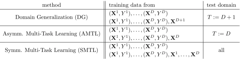
method training data from test domain

Domain Generalization (DG) (X

1_{, Y}1_{), . . . ,(X}D_{, Y}D₎

T :=D+ 1 (X1_{, Y}1_{), . . . ,(X}D_{, Y}D_),XD+1

Asymm. Multi-Task Learning (AMTL) (X

1_{, Y}1_{), . . . ,(X}D_{, Y}D₎

T :=D (X1, Y1), . . . ,(XD, YD),XD

Symm. Multi-Task Learning (SMTL) (X

1_{, Y}1_{), . . . ,(X}D_{, Y}D₎

all (X1_{, Y}1_{), . . . ,(X}D_{, Y}D_),X1_{, . . . ,X}D

Table 1: Taxonomy for domain generalization (DG) and multi-task learning (AMTL and SMTL). Each problem can either be used without (first line) or with (second line) additional unlabeled data.

Another line of work focuses on sharing parameters between tasks. This idea orig-inates in the hierarchical Bayesian literature (Bonilla et al., 2007; Gao et al., 2008). For instance, Lawrence and Platt (2004) introduce a model for MTL in which the mappingfk

in each task k ∈ {1, . . . , D, T} is drawn independently from a common Gaussian Process (GP), and the likelihood of the latent functions depends on a shared parameterθ. A similar approach is introduced by Evgeniou and Pontil (2004): they consider an SVM with weight vectorwk=w0+vk, wherew0 is shared across tasks andvkis task specific. This allows for

tasks to be similar (in which casevkdoes not have a significant contribution to predictions) or quite different. Daum´e III et al. (2010) use a related approach for MTL when there is one source and one target task. Their method relies on the idea of augmented feature space, which they obtain using two features maps Φs_(Xs_{) = (X}s_,Xs_{,0) for the source examples}

and Φt_(Xt_{) = (X}t_,0,Xt_{) for the target examples. They then train a classifier using these}

augmented features. Moreover, they propose a way of using available unlabeled data from the target task at training.

An alternative family of methods is based on learning a set of common features for all tasks (Argyriou et al., 2007a; Romera-Paredes et al., 2012; Argyriou et al., 2007b; Raina et al., 2007). For instance, Argyriou et al. (2007a,b) propose to learn a set of low dimensional features shared between tasks usingL1 regularization, and then learn all tasks independently using these features. In Raina et al. (2007), the authors construct a similar set of features using L1 regularization but make use of only unlabeled examples. Chen et al. (2012) proposes to build shared feature mappings which are robust to noise by using autoencoders.

Finally, the assumption introduced in this paper is based on a causalview on domain adaptation and transfer.

mapping only depend on the distribution of the target variable. Moreover, Zhang et al. (2015a) argue that the availability of multiple domains is sufficient to drop this previous assumption when the distribution ofYkand the conditional Xk|Yk change independently. The conditional in the test task can then be written as a linear mixture of the conditionals in the source domains. The concept of invariant conditionals and exogeneity can also be used for causal discovery (Peters et al., 2016; Zhang et al., 2015b; Peters et al., 2017).

1.3 Contribution

Taking into account causal knowledge,our approachto DG and MTL assumes that covari-ate shift holds only for a subset of the features. From the point of view of causal modeling (Pearl, 2009), assuming invariance of conditionals makes sense if the conditionals represent causal mechanisms (e.g., Hoover, 1990), see Section 2.3 for details. Intuitively, we expect that a causal mechanism is a property of the physical world, and it does not depend on what we feed into it. If the input (which in this case coincides with the covariates) shifts, the mechanism should thus remain invariant (Hoover, 1990; Janzing and Sch¨olkopf, 2010; Peters et al., 2016). In the anticausal direction, however, a shift of the input usually leads to a changing conditional (Sch¨olkopf et al., 2012). In practice, prediction problems are often not causal — we should allow for the possibility that the set of predictors contains variables that are causal, anticausal, or confounded, i.e., statistically dependent variables without a directed causal link with the target variable. We thus expect that there is a

subset S∗ of predictors, referred to as an invariant set, for which the covariate shift as-sumption holds true, i.e., the conditionals of output given predictor Yk|Xk_S∗ are invariant acrossk∈ {1, . . . , D, T}. IfS∗ is a strict subset of all predictors, this relaxes full covariate shift. We prove that knowingS∗ leads to robust properties for DG. Once an invariant set is known, traditional methods for covariate shift can be applied as a black box, see Figure 1. In the MTL setting, when labeled or unlabeled examples from the test task are available during training, we might not want to discard the features outside of S∗ for prediction. Hence, we also propose a method to leverage the knowledge of the invariant set S∗ and the available examples from the test task in order to outperform a method that learns only on the test task.

Finally, note that in this work, we concentrate on the linear setting, keeping in mind that this has specific implications for covariate shift.

1.4 Organization of the paper

Section 2 formally describes our approach and its underlying assumptions; in particular, we assume that an invariant setS∗ is known. For DG, we prove in Section 2.1 that predicting using only features in S∗ is optimal in an adversarial setting. Moreover, we present an example in which we compare our proposed estimator with pooling the training data, a standard technique for DG. In MTL, when additional labeled examples fromT are available, one might want to use all available features for prediction. Section 2.2 provides a method to address this. We discuss a link to causal inference in Section 2.3. Often, an invariant set

2. Exploiting invariant conditional distributions in transfer learning

Consider a transfer learning regression problem with source tasksP1, . . . ,PD, where (Xk, Yk)∼ Pk fork∈ {1, . . . , D}.2 We now formulate our main assumptions.

(A1) There exists a subsetS∗ ⊆ {1, . . . , p} of predictor variables such that

Yk|Xk_S∗ =d Yk 0

|Xk_S0∗ ∀k, k0∈ {1, . . . , D}. (1)

We say that S∗ is an invariant set which leads to invariant conditionals. Here, =d denotes equality in distribution.

(A1’) This invariance also holds in the test taskT, i.e., (1) holds for allk, k0 ∈ {1, . . . , D, T}. (A2) The conditional distribution of Y given an invariant set S∗ is linear: there exists

α∈_R|S∗| _{and a random variable such that for all k∈ {1, . . . , D}, [Y}k_|Xk S∗ =x]

d

=

αtx+k,that is Yk =αtXk_S∗+k, withk⊥⊥Xk_S∗ and for allk∈ {1, . . . , D},k d=.

Assumption (A1’) is stronger than (A1) only in the DG setting, where, of course, (A1’) and (A2) imply the linearity also in the test task T. While Assumption (A1) is testable from training data, see Section 3, (A1’) is not. In covariate shift, one usually assumes that (A1’) holds for the set of all features. Therefore, (A1’) is a weaker condition than covariate shift, see Figure 1. We regard this assumption as a building block that can be combined with any method for covariate shift, applied to the subset S∗. It is known that it can be arbitrarily hard to exploit the assumption of covariate shift in practice (Ben-David et al., 2010). In a general setting, for instance, assumptions about the support of the training distributions P1, . . . ,PD and the test distribution PT must be made for methods such as re-weighting to be expected to work (e.g., Gretton et al., 2009). The aim of our work is not to solve the full covariate shift problem, but to elucidate a relaxation of covariate shift in which it holds given only a subset of the features. We concentrate on linear relations (A2), which circumvents the issue of overlapping supports, for example.

For the remainder of this section, we assume that we are given an invariant subset S∗

that satisfies (A1) and (A2). Note that we will also require (A1’) for DG. In MTL, the invariance can be tested on the labeled data available from the test task, so (A1) and (A1’) are equivalent.

We show how the knowledge of S∗ can be exploited for the DG problem (Section 2.1) and in the MTL case (Section 2.2). Here and below, we focus on linear regression using squared loss

E_PT(β) =_E(XT_,YT_)∼ PT(Y

T _−βt_XT₎2 ₍₂₎

(the superscript T corresponds to the test task, not to be confused with the transpose, indicated by superscriptt). We denote by E_P1_,...,

PD(β) the squared error averaged over the training tasksk∈ {1, . . . , D}.

(A1): ∃S∗⊆ {1, . . . , p}: Y |XS∗ invariant. Covariate shift holds: Y |X{1,...,p} invariant.

Use methods for covariate shift, applied to S∗. Here, (A2): linear model

Figure 1: Assumption (A1) (blue) is a relaxation of covariate shift (orange): the covariate shift assumption is a special case of (A1) withS∗ ={1, . . . , p}. Given the invariant setS∗, methods for covariate shift can be applied.

2.1 Domain generalization (DG): no labels from the test task

We first study the DG setting in which we receive no labeled examples from the test task during training time. Throughout this subsection, we assume that additionally to (A1) and (A2), assumption (A1’) holds. It is important to appreciate that (A1’) is a strong assumption that is not testable on the training data: it is an assumption about the test task. We believe no nontrivial statement about DG is possible without an assumption of this type.

Now, we introduce our proposed estimator, which uses the conditional mean of the target variable given the invariant set in the training tasks. We prove that this estimator is optimal in an adversarial setting.

Proposed estimator. The optimal predictor obtained by minimizing (2) is the condi-tional mean

βopt:= arg min

β∈Rp

E

PT(β), (3)

which is not available during training time. Given an invariant setS∗ satisfying (A1), (A1’) and (A2), we propose to use the corresponding conditional expectation as an estimator. In other words, let βS∗ = arg min_β∈

R|S∗|(Y

1_−βt_X1

S∗)2 be the vector obtained by minimizing the squared loss in the training tasks using only predictors inS∗. We propose as a predictor the vector βCS(S∗) ∈_Rp _{obtained by adding zeros to β}S∗ _{in the dimensions corresponding}

to covariates outside of S∗. More formally, we propose to use as a predictor

Rp → R

x 7→ _E[Y1|X1_S∗ =x_S∗] and write E[Y

1_|X1

S∗=x_S∗] = βCS(S ∗_)t

x. (4)

Because of (A1), the conditional expectation in (4) is the same in all training tasks. In the limit of infinitely many data, given a subset S, βCS(S) is obtained by pooling the training tasks and regressing using only features in S. In particular, βCS := βCS({1,...,p}) is the estimator obtained when assuming traditional covariate shift.

Theorem 1 (Adversarial) Consider (X1, Y1) ∼ _P1_{,. . ., (X}D_{, Y}D_{) ∼}

PD and an

invari-ant set S∗ satisfying (A1) and (A2). The proposed estimator satisfies an optimality state-ment over the set of distributions such that (A1’) holds: we have

βCS(S∗) ∈arg min

β∈_Rp

sup

PT∈P

E_PT(β),

where βCS(S∗) is defined in (4) and P contains all distributions over (XT, YT), T =D+ 1, that are absolutely continuous with respect to the same product measure µ and satisfy

YT |XT_S∗

d

=Y1|X1_S∗.

Unlike the optimal predictor βopt, the proposed estimator (4) can be learned from the data available in the training tasks. Given a sample (Xk

1, Y1k), . . . ,(Xknk, Y

k

nk) from tasks

k∈ {1, . . . , D}, we can estimate the conditional mean in (4) by regressingYkon Xk_S∗. Due to (A1), we may also pool the data over the different tasks and use

(X1₁, Y₁1), . . . ,(X1_n1, Y_n1₁),(X2₁, Y₁2), . . . ,(XD_n D, Y

D nD)

as a training sample for this regression.

One may also compare the proposed estimator with pooling the training tasks, a stan-dard baseline in transfer learning which corresponds to assuming that usual covariate shift holds. Focusing on a specific example, Proposition 2 in the following paragraph shows that when the test tasks become diverse, predicting using (4) outperforms pooling on average over all tasks.

Comparison against pooling the data. We proved that the proposed estimator (4) does well on an adversarial setting, in the sense that it minimizes the largest error on a task inP. The following result provides an example in which we can analytically compare the proposed estimator with the estimator obtained from pooling the training data, which is a benchmark in transfer learning. We prove that in this setting, the proposed estimator outperforms pooling the data on average over test tasks when the tasks become more diverse. Let Xk_S∗ be a vector of independent Gaussian variables in task k. Let the target Yk satisfy

Yk=αtXk_S∗+k, (5)

where for each k ∈ {1, . . . , D}, k _{is Gaussian and independent of X}k

S∗. We have Xk = (Xk_S∗, Zk), where

Zk=γkYk+ηk,

for someγk∈_Rand whereηk is Gaussian and independent ofYk.3 _{Moreover, assume that}

the training tasks are balanced. We compare properties of estimator βCS(S∗) _{defined in}

Equation (4) against the least squares estimator obtained from pooling the training data. In this setting, the tasks differ in coefficientsγk, which are randomly sampled. We prove that the squared loss averaged over unseen test tasks is always larger for the pooled approach, when coefficientsγkare centered around zero. In the case where they are centered around a non-zero mean, we prove that when the variance between tasks (in this case, for coefficients

γk) becomes large enough, the invariant approach also outperforms pooling the data.

1 2 3 4 5 6 7

Σ2 0

2 4 6 8 10 12 14

Expected

error

on

test

task

Pooled Subsets

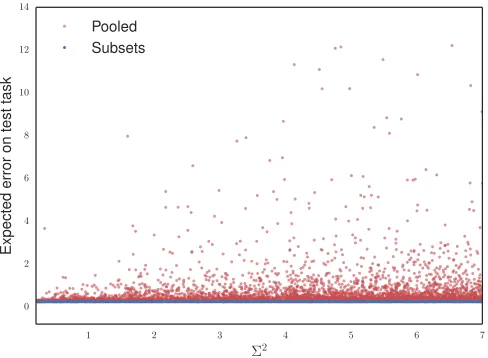
Figure 2: The figure shows expected errors for the pooled approach and the proposed method, see Equation (6). µ= 0. We consider two training tasks over 10,000 simulations. In each, we randomly sample the variance of each covariate in X, the variance of η, and γ.

σ2 is the same in all tasks. As predicted by Proposition Proposition 2 observe that the error from the pooled approach (red) is systematically higher than the error from the prediction using only the invariant subset (blue), and both the error and its variance become large as the variance Σ2 _{of coefficientsγ}k _increases.

Proposition 2 (Average performance) Consider the model described previously. More-over, assume that the tasks differ as follows: the coefficientsγ1, . . . , γD, γT =γD+1 are i.i.d. with mean zero and variance Σ2 _{>0. The tasks do not differ elsewhere. In particular, the} distribution of Xk

S∗ is the same for all tasks. Then the least squares predictor obtained from

pooling theD training tasks βCS= (β_SCS∗ , βCS_Z ) satisfies:

EγT E

PT β

CS

≥_EγT

E

PT

βCS(S∗)

=σ2. (6)

In particular, this implies the following:

Eγ1_,...,γD_,γT E

PT β

CS

≥Eγ1_,...,γD_,γT

E_PT

βCS(S∗)

=σ2. (7)

Moreover, if the coefficients γ1, . . . , γD, γT are i.i.d. with non-zero mean µ, (6) holds for fixed γ1, . . . , γD if Σ2 _{≥P(µ), where P is a polynomial in µ, see Appendix A.2 for details.}

The proof of Proposition 2 can be found in Appendix A.2. Figure 2 visualizes Proposition 2 for two training tasks, it shows the expected errors for the pooled and invariant approaches, see (6), as the variance Σ2 _{increases. Recall that Σ}2 _{corresponds to the variance of}

zero, γk is close to zero in all tasks, which explains the equality of both the pooled and invariant errors for the limit case Σ approaching 0. For coefficients γk centered around a non zero value, Equation (6) does not necessarily hold for small Σ2_.

Proposition 2 presents a setting in which the invariant approach outperforms pooling the data when the test errors are averaged overγ, i.e.,EγT E

PT β

CS

≥EγT E

PT β

CS

. It is also clear to see that the equality of the distribution of k in Equation (5) for all

k ∈ {1, . . . , D} leads to Varγ E_PT βCS(S

∗₎

= 0, thus our invariant estimator minimizes the variance of the test errors across all related tasks.

2.2 Multi-task learning (MTL): combining invariance and task-specific information

In MTL, a labeled sample XT i , YiT

nT

i=1 is available from the test task and the goal is to

transfer knowledge from the training tasks. As before, we are given an invariant set S∗

satisfying (A1) and (A2). Can we combine the invariance assumption with the new labeled sample and perform better than a method that trains only on the data in the test task? According to (A1) and (A2), the target satisfiesYk=αtX_Sk∗+k, where the noise k has zero mean and finite variance, is independent of Xk_S∗ and has the same distribution in the different tasks k ∈ {1, . . . , D, T}. Our objective is to use the knowledge gained from the training tasks to get a better estimate of βopt defined in Equation (3). We describe below a way to tackle this using missing data methods.

Missing data approach In this section, we specify how we propose to tackle MTL by framing it as a missing data problem. While the idea is presented in the context of AMTL, it can be used for SMTL in the same way. In order to motivate the method, assume that for each k ∈ {1, . . . , D, T}, there exists another probability distribution Qk with density

qk having the following properties: (i) when restricted to (Xk_S∗, Yk),Qk coincides with Pk, (ii) the conditional qT(y|xS∗,x_N) coincides with pT(y|x_S∗,x_N) on the test task and (iii)

q(y|xS∗,x_N) := qk(y|x_S∗,x_N) is the same in all tasks (which is not satisfied by _Pk, of course). The goal of learning the regression model fromY onXS∗ and X_N in_PT coincides with the task of learning the same regression model in QT. Property (iii) implies that we can pool the data from all tasks Qk. This is not possible, of course, for the given data, which we have received from the distributions Pk. But now assume that in all training tasks, we only have access to the marginal (Xk_S∗, Yk) from_Qk. Any method that addresses the regression under these constraints be used with the data available because of (i). We first prove the existence of such distributions Qk:

Proposition 3 (Correctness of transfer) LetS∗ be an invariant set verifying (A1) and (A2). Fork∈ {1, . . . , D, T}, denote by(x, y)7→pk_{(x, y)the density of}

Pk. Then there exists

a function q:Rp →R+ such that for eachk∈ {1, . . . , D, T}, there exists a distribution Qk

with density qk such that for all (x, y)∈_Rd+1_{, for all k∈ {1, . . . , D, T},} i) qk(xS∗, y) =pk(x_S∗, y),

ii) qT(y|xS∗,x_N) =pT(y|x_S∗,x_N),

iii) qk(y|xS∗,x_N) =q(y|x_S∗,x_N).

taskk∈ {1, . . . , D, T} come from Qk. Note that some of the data are only missing for the training tasks. More precisely, Xk_N is missing for k ∈ {1, . . . , D}, while because of (i) in Proposition 3, (Xk_S∗, Yk) is available for all tasks k∈ {1, . . . , D, T}. We thus pool the data and learn a regression model of Y versus (XS∗,X_N) by maximizing the likelihood of the observed data.

We formalize the problem as follows. Let (Zi)ni=1 = (XS∗_,i,X_N,i, Y_i)n

i=1 be a pooled

sample of the available data from the training tasks and the test task, in which XN,i is

considered missing ifXi is drawn from one of the training tasks. Here,n=PTk=1nk is the

total number of training and test examples. Denote byZobs,ithe components ofZiwhich are

not missing. In particular,Zobs,i=Ziifiis drawn from the test task andZobs,i= (XS∗_,i, Y_i) otherwise. Moreover, let Σ be a (p+ 1)×(p+ 1) positive definite matrix, and Σi is the

submatrix of Σ which corresponds to the observed features for example i. If example i is drawn from a training task, Σi is of size (|S∗|+1)×(|S∗|+1), and (p+1)×(p+1) otherwise.

The log-likelihood based on the observed data for matrix Σ satisfies:

`(Σ) = const−1

2

n

X

i=1

det (Σi)−

1 2Z

T obs,iΣ

−1

i Zobs,i, (8)

and our goal is to find Σ which maximizes (8). This model for the likelihood assumes that the data is multi-variate Gaussian with covariance matrix Σ.

When all data are observed, the least squares estimatorβopt can be seen as the result of a two step procedure. First, (8) is maximized for the sample covariance matrix. Then, one computes the conditional meanE[Y |X=x] of the estimated joint distribution of (X,Y). In the case of missing data, however, the sample covariance matrix does no longer maximize (8), see paragraph ‘A naive estimator for comparison’ below. Instead, we maximize (8) using EM.

Chapter 11 in Little and Rubin (1986) provides the update equations for optimizing Equation (8) using EM. More precisely, given an estimate Σr _{of the covariance matrix at}

step r, the algorithm goes as follows. E step: For an example i, we define

Zr_i := (

Zi if exampleiis from the test task,

(XS∗_,i,_E(Xr

N|Zobs,i), Yi) otherwise.

Here, we are essentially imputing the data forXN in the training tasks by the conditional

mean given the observed data, using the current estimate of the covariance matrix Σr_.

The conditional expectation is computed using the current estimate Σr _{and the Gaussian}

conditioning formula:

E(XrN|Zobs,i) = ΣrN Zobs(Σ

r Zobs)

−1 Zobs,i,

where Σr

N Zobs is the submatrix of Σ

r _{corresponding to the cross-covariance between X} N

and (XS∗, Y), and Σr

Zobs is the submatrix corresponding to the covariance of (XS∗, Y). For

examples from the test task, we simply copy the example, sincePT =QT. Moreover, define

C_N,ir := (

0 if exampleiis from the test task,

M step: compute the sample covariance given the imputed data:

Σr+1 = 1

nE n

X

i=1

Zr_i(Zr_i)t|Zobs,i,Σr !

= 1

n n

X

i=1

Zr_i(Zr_i)t+C_ir,

whereC_iris a (p+1)×(p+1) matrix whose submatrix corresponding to features inN isC_N,ir , and the remaining elements are 0. The intuition for the M step is simple: we compute the sample covariance with the values imputed forXN. Since these values are being imputed,

matrixC adds uncertainty for the corresponding values.

Once the algorithm has converged, we can read off the regression coefficient from the joint covariance matrix as E[Y |XS∗ = x_S∗]. The whole procedure is initialized with the sample covariance matrix computed with the available labeled sample fromT.

Incorporating unlabeled data The previous method also allows us to incorporate un-labeled data from the test task. Indeed, assume that an unun-labeled sampleXT = (XT_S∗,XT_N) from the test task is also available at training time. This can be incorporated in the pre-vious framework since the label Y can be considered to be missing (as opposed to XT_N previously). We can then write Zr_i = (XS∗,i,XN,i,_E(Yr

i |Zobs,i)) for the unlabeled data,

thus imputing the value of Y in in the E-step by the conditional mean given (XS∗_,i,X_N,i). The added covariance is then C_Y,ir = Var(Y)r_−Σr

Y Zobs(Σ

r Zobs)

−1_Σr

ZobsY. The rest of the

algorithm remains unchanged.

A naive estimator for comparison In the population setting, Proposition 5 in Ap-pendix A.4 provides an expression forβopt as a function ofα and from Assumption (A2). As in the previous paragraph, one could try to estimate the covariance matrix of (X, Y) using the knowledge of α and from the training tasks, and then read off the regression coefficients. In the presence of a finite amount of labeled and unlabeled data from the test task, a naive approach would thus plug in the knowledge ofα and as follows: the entries of ˆΣX,Y that correspond to the covariances betweenXS∗ andY are replaced with ˆΣ_X

S∗·α,

and the entry corresponding to the variance of Y is replaced by αtΣˆXS∗α+ Var(). This,

however, often performs worse than forgetting aboutαand using the data in the test domain only, see Figure 5 (left). Why is this the case? The naive solution described above leads to a matrix Σ that does not onlynotmaximize (8) but that often is not even positive definite. One needs to optimize over the free parameters of Σ, which corresponds to the covariance betweenXN and Y, given the constraint of positive definiteness. For comparison, we

mod-ified the naive approach as follows. First, we find a positive definite matrix satisfying the desired constraints. In order to do this, we solve a semi-definite Program (SDP) with a trivial objective which always equals zero. Then, we maximize the likelihood (8) over the free parameters of Σ with a Nelder-Mead simplex algorithm. The constrained optimiza-tion problem can be shown to be convex in the neighborhood of the optimum (Zwiernik et al., 2017, Sec. 3) if the number of data in the test domain grows. While gradients can be computed for this problem, gradient-based methods seem to perform poorly in practice (experiments are not shown for gradient based methods).

In an idealized scenario, infinite amount of unlabeled data in the test and labeled data in the training tasks could provide us with ΣX, Σ(XS∗,Y) and Var(Y). We could then plug

Figure 5 (left). In practice, we have to estimate ΣX, Σ(XS∗,Y)and Var(Y) from data. Thus,

the EM approach mentioned above constitutes the more principled approach.

2.3 Relation to causality

In this section, we provide a brief introduction to causal notions in order to motivate our method. More specifically, we show that under some conditions, the setS∗ of causal parents verifies Assumptions (A1) and (A1’). Structural equation models (SEMs) (Pearl, 2009) are one possibility to formalize causal statements. We say that a distribution over random variables X = (X1, . . . , Xp) is induced by a structural equation model with corresponding

graph G if each variable Xj can be written as a deterministic function of its parentsPAG_j (inG) and some noise variableNj:

Xj =fj(X_PAG

j, Nj), j= 1, . . . , p . (9)

Here, the graph is required to be acyclic and the noise variables are assumed to be jointly independent. An SEM comes with the ability to describe interventions. Intervening in the system corresponds to replacing one of the structural equations (9). The resulting joint distribution is called an intervention distribution. Changing the equation for variable Xj

usually affects the distribution of its children for example, but never the distribution of its parents. Consider now an SEM over variables (X, Y). Here, we do not specify the graphical relation between Y and the other nodes: Y may or may not have children or parents. Suppose further that the different tasks P1, . . . ,PD are intervention distributions of an underlying SEM with graph structureG. If the target variable has not been intervened on, then the set S∗ := PAG_Y satisfies Assumptions (A1) and (A1’). This means that as long as the interventions will not take place at the target variable, the set S∗ of causal parents will satisfy Assumptions (A1) and (A1’).

Recently, Peters et al. (2016) have given several sufficient conditions for the identifiability of the causal parents in the linear Gaussian framework. E.g., if the interventions take place at informative locations, or if we see sufficiently many different interventions, the set of causal parents is the only set S∗ that satisfies Assumptions (A1) and (A1’). If there exists more than one set leading to invariant predictions, they consider the intersection of all such subsets. In this sense, seeing more environments helps for identifying the causal structure. In this work, we are interested in prediction rather than causal discovery. Therefore, we try to find a trade-off between models that predict well and invariant models that generalize well to other domains. That is, in the DG setting, we are interested in the subset which leads to invariant conditionals and minimizes the prediction error across training tasks.

If the tasks Pk correspond to interventions in an SEM, we may construct an extended SEM with a parent-less environment variable E that points into the intervened variables. Then,Pk equals the distribution of (X, Y)|E =k, see (Peters et al., 2016, Appendix C). If the distribution of (X, Y, E) is Markov and faithful w.r.t. the extended graph, the smallest set S that leads to invariant conditionals and to best prediction is a subset of the Markov blanket of Y: certainly, it contains all parents of Y; if it includes a descendant of Y, this must be a child of Y (which yields better prediction and still blocks any path from Y to

3. Learning invariant conditionals

In the previous section, we have seen how a known invariant subset S∗ ⊆ {1, . . . , p} of predictors leading to invariant conditionalsYk|Xk_S∗, see Assumptions (A1) and (A1’), can be beneficial in the problems of DG and MTL. In practice, such a set S∗ is often unknown. We now present a method that aims atinferring an invariant subset from data. Throughout this paper, we denote bySany subset of features, whileS+ is an invariant set (which is not necessarily unique) for which (A1) holds. Such a subsetS+does not necessarily satisfy both Assumptions (A1) and (A1’). Indeed, in DG, only (A1) is testable in the training data. More precisely, if several invariant sets which satisfy (A1) are found, and only some of them satisfy (A1’), we cannot find these from data. We therefore have to add a criterion allowing us to select among several invariant sets. The method we propose provides an estimator ˆS

for an invariant subsetS+, which is chosen as the subset satisfying Assumption (A1) which maximizes predictive accuracy on a validation set. In MTL, we still write S+, even if we could then write S∗ as (A1’) becomes testable. It is summarized in Algorithm 1, code is provided inhttps://github.com/mrojascarulla/causal_transfer_learning.

3.1 Our method.

Algorithm 1:Subset search Inputs: Sample (xk_i, yk_i)nk

i=1 for tasks k∈ {1, . . . , D}, threshold δ for independence

test.

Outputs: Estimated invariant subset ˆS.

1 Set Sacc={}, MSE ={}. 2 for S⊆ {1, . . . , p}do

3 linearly regressY onX_S and compute the residuals R_βCS(S) on a validation set.

4 computeH= HSICb

(R_βCS(S)_,i, Ki)n_i=1

and the corresponding p-valuep∗ (or the p-value from an alternative test, e.g., Levene test.).

5 if p∗ > δthen

6 computeEb

P1,...,D(β

CS(S)_{), the empirical estimate of E}

P1,...,D(β

CS(S)_{) on a}

validation set.

7 S_acc.add(S), MSE.add(Eb

P1,...,D(β

CS(S)₎₎ 8 end

9 end

10 Select ˆS according to RULE, see Section 3.4.

Consider a set ofDtasks, a target variableYk and a vectorXkof ppredictor variables in taskk. Forβ ∈Rp, we define the residual in task k as:

Rk_β =Yk−βtXk, k∈ {1, . . . , D}. (10)

By Assumptions (A1) and (A2), there exists a subsetS+and some vectorβCS(S+)such that for allj /∈S+,β_jCS(S+) = 0 andR1

βCS(S+) d

=. . .=d RD

βCS(S+). Such a setS+is not necessarily

Algorithm 2:Greedy subset search Inputs: Sample (xk_i, yk_i)nk

i=1 for tasks k∈ {1, . . . , D}, threshold δ for independence

test.

Outputs: Estimated invariant set ˆSgreedy.

1 Set Sacc={}, ˆScurrent{}, MSE ={}. 2 for i∈ {1, . . . , n_iters} do

3 Setstatmin=∞.

4 forS∈ S_Sˆ

current do

5 linearly regressY on X_S and compute the residuals R_βCS(S) on a validation

set.

6 computeH = HSIC_b

(R_βCS(S)_,i, Ki)n_i=1

and the corresponding p-valuep∗

(or the p-value from an alternative test, e.g. Levene test.).

7 if p∗ > δthen

8 computeEb

P1,...,D(β

CS(S)_{), the empirical estimate of E}

P1,...,D(β

CS(S)_{) on a}

validation set.

9 S_acc.add(S), MSE.add(Eb

P1,...,D(β

CS(S)_)), 10 set ˆS_current =S.

11 end

12 else if H < statmin then

13 set ˆS_current =S,stat_min =H.

14 end

15 end 16 end

17 Select ˆS according to RULE, see Section 3.4.

different tasks are observed at training time. We propose to do an exhaustive search over subsetsSof predictors and statistically test for equality of the distribution of the residuals in the training tasks, see the section below. Among the accepted subsets, we select the subset ˆS

which leads to the smallest error on a validation set. This is a fundamental difference to the method proposed by Peters et al. (2016). Indeed, while our method addresses the transfer problem, Peters et al. (2016) is about causal discovery. Algorithm 1 finds an invariant subset which also leads to the lowest validation error. This subset may contain covariates which are non causal, see Section 4.3 for further details. On the other hand, Peters et al. (2016) estimate the causal parents (with coverage guarantee). Such an approach has a different purpose and performs very badly both in DG and MTL: e.g., when all tasks are identical, it uses the empty set as predictors, while our method selects the full set of predictors.

3.2 Statistical tests for equality of distributions.

In order to test whether a subsetS leads to invariant conditionals, we can use a statistical test to check whether the residuals Rk_βCS(S) have the same distribution in all tasks k ∈ {1, . . . , D}. We propose two possible methods.

For Gaussian data, one can use a Levene test (Levene, 1960) to test whether the residuals have the same variance in all tasks; their means are zero as long as an intercept is included in the regression model.

As an alternative, we propose a nonparametric D-sample test by testing whether the residuals are independent of the task index. This test is a direct application of HSIC (Gret-ton et al., 2007) but to our knowledge, is novel. Suppose that the index of the task can be considered as a random variable K. We consider the sample Z = (R_βS_,i, K_i)n_i=1 as

drawn from a joint distribution over residuals and task indices, where n = PD

k=1nk and

Ki ∈ {1, . . . , D} is a discrete value indicating the index of the corresponding task. The residuals have the same distribution in all training tasks if and only ifR_βS and K are

inde-pendent. Two characteristic kernels are used: a kernelκis used for embedding the residuals and a trivial kernel d such that d(i, j) = δij is used for K. Let therefore HSIC(R_βS, K)

denote the value of the HSIC (Gretton et al., 2007) betweenR_βS andK, and let HSIC_b(Z)

be the corresponding test statistic. A subsetS is accepted if if leads to accepting the null hypothesis of independence between R_βS and K at levelδ.

Both in the case of the Levene test and the D-sample test, the test outputs a p-value

p∗, and we accept the nullH0 ifp∗ > δ. Among these accepted subsets, we output the set ˆS

which leads to the smallest loss on a validation set. The test levelδ is given as an input to our method and allows for a trade-off between predictive accuracy and exploiting invariance. Asδ tends to zero, the null is accepted for all subsets and we then select all features, which is equivalent to covariate shift. Whenδ approaches one, no subset is accepted as invariant. Our method then reduces to the mean prediction. In order to compute p-values, a Gamma approximation is used for the distribution of HSICb(Z) under the null.

For non-additive models, one may even apply a conditional independence test (e.g., Zhang et al., 2011; Fukumizu et al., 2008) to test whether K is independent of Y |XS.

3.3 Scalability to a large number of predictors

When the number of features p is large, full subset search is computationally not feasible. We propose two solutions for this scenario. If one has reasons to believe that the signal is sparse, that is the true setS∗is small, one may use avariable selectiontechnique such as the Lasso (Tibshirani, 1996) as a first step. Under the assumptions described in Section 2.3, we know that the invariant set with the best prediction in the training tasks can be assumed to be a subset of the relevant features (which here equals the Markov blanket ofY). Thus, if variable screening is satisfied ,i.e., one selects all relevant variables and possibly more, the pre-selection step does not change the result of Algorithm 1 in the limit of infinitely many data. For linear models with `1 penalization, variable screening is a well studied problem,

see, e.g., compatibility and βmin conditions (B¨uhlmann and van de Geer, 2011, Chapter 2.5).

X1 X2

X3

Y X5

Figure 3: Example of a directed acyclic graph, see Section 2.3. If Y is not intervened on, the conditional Y |X1, X2, X3 remains invariant.

removing exactly one predictor inS. If no subset has been accepted at a given iteration, we select the neighbor leading to the smallest test statistic. If a neighbor is accepted, we select the one which leads to the smallest training error. We start with the p subsets with only one element, and allow to add or remove a single predictor at each step, see Algorithm 2. As often for greedy methods, there is no theoretical guarantee.

3.4 Subset selection in MTL

In DG, among the accepted subsets, we select the set ˆS which leads to the lowest validation error. In MTL, however, a labeled sample from the test task T is available at training time. Therefore, Algorithm 1 is slightly modified. First, we get all the sets for which

H0 is accepted. Then, we select the accepted set ˆS which leads to the smallest 5 fold

cross validation error. For each subset, we compute the least squares coefficients using the procedure described in Section 2.2, and measure the prediction error on the held out validation set. Using the notation of Algorithm 1, letSaccbe the set of subsets accepted as

invariant, and let M SE be the set of their corresponding squared errors on the validation set. The following rules are used for selecting an invariant set in DG and MTL.

i) RULE for DG: Return ˆS =Sacc[arg min MSE].

ii) RULE for MTL: Define CVacc = {}. For each set S ⊆ Sacc, do CVacc.add(CVS),

whereCVS is the 5-fold cross validation error over the labeled test data obtained by optimizing (8) using EM with subsetS.

Return ˆS=Sacc[arg minCVacc].

Given a set of k∈ {1, . . . , T} training tasks, a collection of sets ˆS1, . . . ,Sˆu (eventually

estimator description

βCS(cau) Linear regr. with true causal predictors (often unknown in practice).

βCS( ˆS) _{Finding the invariant set ˆS using full subset search and performing lin. regr. using}

predictors in ˆS. ˆSgreedy corresponds to finding the invariant set using a greedy procedure. SLassoˆ corresponds to doing variable selection using Lasso as a first step, then doing full subset search on the selected features.

βCS _{Pooling the training data and using linear regr.}

βCS( ˆS+) _{Finding the invariant set ˆSusing full subset search and solve the optimization problem}

described in ’A naive estimator for comparison’.

βCS( ˆS]) Finding the invariant set ˆS using full subset search and maximizing (8) for MTL using EM.

βmean _{Pooling the training data and outputting the mean of the target.} βdom _{Linear regression using only the available labeled sample fromT.} βM T L _{Multi-task feature learning estimator (Argyriou et al., 2007a).} βDICA _{DICA (Muandet et al., 2013) with rbf kernel.}

βmDA _{Pooling the training data and an unlabeled sample from T, learning features using} mSDA (Chen et al., 2012) with one layer and linear output, then using linear regr.

Table 2: Estimators used in the numerical experiments. A ’+’ next to a subsetScorresponds to the method for MTL described in the last paragraph of Section 2.2.

4. Experiments

We compare our estimator to different methods, which are summarized in Table 2. βCS(cau)

uses the ground truth for S∗ when it is available, βCS( ˆS) corresponds to full search us-ing Algorithm 1, βCS uses the pooled training data, βM T L performs the Multi-task fea-ture learning algorithm (Argyriou et al., 2007a) for the MTL setting and βDICA _performs

DICA (Muandet et al., 2013) for DG. For DICA, which is a nonlinear method, the kernel matrices are constructed using an rbf kernel, and the length-scale of the kernel is selected according to the median heuristic. In the MTL setting, we combine the invariance with task specific information by optimizing (8) using EM, resulting in regression coefficients

βCS( ˆS]) andβCS(cau]) when the ground truth is known. Finally,βCS(cau],U L) indicates that unlabeled data from T was also available. For reference, Figure 5 (left) provides results for βCS( ˆS+) and βCS(cau+), which correspond to the estimators obtained by solving the constrained optimization problem described in the paragraph ‘A naive estimator for com-parison’ of Section 2.2 (βCS(cau+)uses the ground truth forS∗ andα), whileβnaive imputes the covariance matrices but does not optimize the free parameters. βCS(cau+,i.d.) (infinite data) also assumes that we know the ground truth for the entries of the covariance matrix for the test task corresponding to the covariance of X, the covariance betweenXS∗ andY, and the variance of Y.

4.1 Synthetic data set

models in Algorithms 1 and 2, and the remaining data as validation. The sensitivity to the choice ofδ is discussed in Section 4.2.

Generative process of the data For each taskk∈ {1,2, . . . , D, T}, we sample a set of causal variables from a multivariate Gaussian

Xk_S∗ ∼ N(0,Σk_S∗)

where the covariance matrix Σk

S∗ is drawn from a Wishart distribution W(U_Sk∗, p), where

Uk

S∗ is computed as Vk(Vk)t. Here, Vk is a (|S|,|S|) matrix of standard Gaussian random variables.

The target variable Yk is drawn as

Yk =αXk_S∗+k

where k ∼ N(0,2) (the standard deviation of k is 6 for the non sparse DG experiment with 30 predictors, see the bottom of Figure 4).

We sample the remaining predictor variables as

Xk_N =γkYk+βk(Xk_S∗)_C+ηk

whereηk∼ N(0,Σk

N). (XkS∗)C is a subset ofXk_S∗of size|C|which generates both the target

Yk and XNTk. γk of size |N| is computed asγk= (1−λ)γ0+λgk, where λ∈[0,1], γ0 is

the same in all tasks whilegk _{is task dependent. Bothγ}

0 andgkare drawn from a standard

Gaussian. Similarly to γk,βkis a (|C|,|N|) matrix computed asβk= (1−λ)β0+λbk. Σk_N

is sampled similarly to Σk

S∗. Finally,α is sampled from a standard Gaussian distribution. The generative process and hyper-parameters are the same for all the experiments (DG and MTL).

Results Our goal is to linearly predict target YT using predictors XT = (XT_S∗,XT_N) on the test task. Given regression coefficient β, we measure the performance in the test task using the logarithm of the empirical estimator of E

PT(β).

In Figure 4, we are in the DG setting (thus, no labeled examples from T are observed at training). 4000 examples per training task are available for the top left and right plots, while only 1000 examples per task are available on the bottom because of computational reasons. We report the log average empirical MSE over left out test tasks. We study both sparse and non sparse settings (in which full search is not feasible). On the upper left and upper right, we see that when more than four training tasks are available, both the full search and greedy approaches are able to recover an invariant set, and outperform pooling the data for any number of training tasks. When more than five training tasks are observed,

βCS( ˆS) _{performs like β}CS(cau)_{, which uses knowledge of the ground truth. On the bottom,}

full search is not feasible, andβCS( ˆSgreedy) outperforms other approaches.

2 3 4 5 6 # of training tasks T

1.0 1.5 2.0 2.5 3.0 3.5 4.0

log

MS

E

CS CS(S)

CS(Sgreedy)

CS(cau)

mean mSDA

DICA

2 3 4 5 6

# of training tasks T 1.0

1.5 2.0 2.5 3.0 3.5 4.0

log

MS

E

CS CS(S)

CS(Sgreedy)

CS(cau)

mean mSDA

DICA

2 3 4 5 6 7 8 9 10 11 # of training tasks T

3.6 3.8 4.0 4.2 4.4

log

MS

E

CS CS(Sgreedy)

CS(cau) mean

mSDA DICA

Figure 4: DG setting. Logarithm of the empirical squared error in the test task for the different estimators in the DG setting. The results show averages and 95% confidence intervals for the mean performance over 100 repetitions. We vary the number of tasks

D available at training time. Upper left: both S and N are of size 3, such that X is 6-dimensional. |C|is of size one. Upper right: 30 noise variables are added to X. Variable selection using the Lasso is used prior to computing βCS( ˆS), while βCS( ˆSgreedy) uses all predictors. Bottom: both S and N are of size 15. Full search is not computationally feasible in this setting and only the greedy procedure can be used. Other methods such asβCS,βmSDA and βDICA often perform badly, which explains why in comparison βmean

appears to performs well.

0 20 40 60 80 Number of labeled examples in T 0.0 0.1 0.2 0.3 0.4 0.5 0.6 0.7 0.8

Percentage of simulations in whic

h

do

m is

ou tp er fo rm ed

Reference:

CS(cau + , id)

CS(cau + ) naive

CS(S + )

0 1000 2000 3000 4000 5000

Number of unlabeled examples in T 0.0 0.1 0.2 0.3 0.4 0.5 0.6 0.7

Percentage of simulations in which

CS

(ca

u

) is ou

tp

er

fo

rm

ed

Reference:

mSDA CS(cau UL)

100 300 500 700 900

# of training tasks T 10 8 6 4 2 0 log MS E CS dom mSDA CS(cau ) CS(S ) MTL

0 200 400 600 800

Number of labeled examples in T 0.0

0.2 0.4 0.6 0.8

Percentage of simulations in whic

h

do

m is

ou tp er fo rm ed

Reference:

CS mSDA

CS(cau ) CS(S )

MTL

Figure 5: MTL setting. Percentage of repetitions (out of 100) for which the corresponding method outperformsβdom (orβCS(cau]) for the top right plot). BothS and N are of size 3, such thatXis 6-dimensional. Upper left: AMTL setting. This plot shows that the methods

βCS( ˆS+)and βCS(cau+)presented in Section 2.2 perform well, but a large amount of data is necessary: 50000 unlabeled examples fromT and 36000 training examples are available. The naive methodβnaive performs poorly. Upper right: in the SMTL setting, we fix the number of training data (500 per task) and vary the amount of unlabeled data available from the test task. We report the percentage of scenarios in which the corresponding method outperforms

βCS(cau])this time (which uses no unlabeled data). WhileβmDAalways performs worse than

βCS(cau]) and does not exploit the unlabeled data, we see thatβCS(cau],U L) performs better as the amount of unlabeled data increases. Bottom: SMTL setting, and we vary the number of labeled examples available in each training task. Here, significantly less labeled data was available in the training tasks (from 50 to 1000 per task). In this setting, the methods using unlabeled data were given 100 unlabeled examples. Bottom left: logarithm of the empirical squared error in the test task for different estimators. Bottom right: percentage of repetitions (out of 100) for which the corresponding method outperformsβdom.

avail-0.000 0.002 0.004 0.006 0.008 0.010 0.012 0.014

(

_{) (}

₎

0 10 20 30 40 50 60 70

Number of repetitions

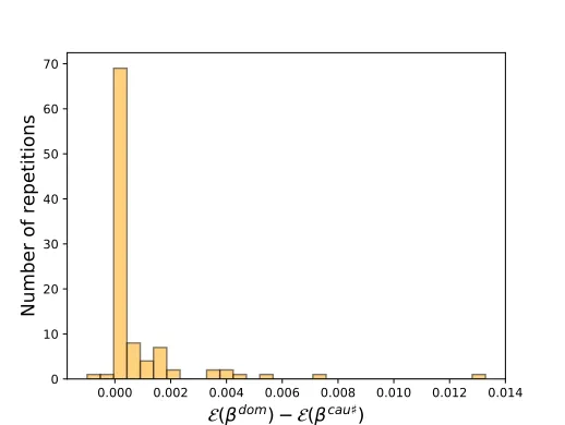
Figure 6: In the SMTL setting, 900 examples from each of the training tasks are available (this corresponds to the data point furthest to the right in the bottom plot of Figure 5). We run 100 repetitions and plot the histograms of ∆ = E(βdom) − E(βCS(cau])). The proposed estimator outperform βdom: for a large proportion of the repetitions, ∆ > 0. More importantly, the distribution of ∆ is heavily skewed in the positive values. In other words, when βdom outperformsβCS(cau]), the difference in performance is small, while the difference is often larger for the converse.

able, and only few labeled examples are available in each task. Here, we see thatβCS(cau]),

βCS( ˆS]) and βM T L perform well, while other methods do not. In terms of MSE (bottom left), the difference in performance between the top competing methods is not statistically significant.

Time complexity The most expensive component of our method is the estimation of the invariant subset. In the DG experiment in Figure 4, with n= 4000 examples available for each of the 6 tasks, andp= 6 predictors, full subset search takes 0.067 seconds and greedy search 0.037, where the results are averaged over 100 repetitions. With p= 10, full search averages at 1.57 seconds, and greedy search 0.0396. With p= 30, where full search is not feasible, greedy search averages at 1.21 seconds. In the MTL experiment in Figure 5, the EM algorithm runs for 0.00105 seconds on average over 100 repetitions. As a reference, in MTL, linear regression averages at 0.000301 seconds and mSDA at 0.0547 seconds.

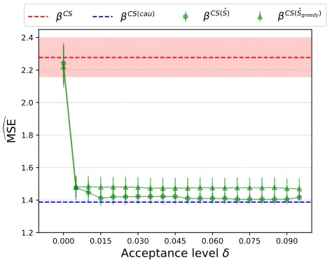
4.2 Sensitivity to the acceptance level δ

Both Algorithm 1 and its greedy version Algorithm 2 receive an acceptance levelδ as input for the statistical test. In our other experiments, we chose the standard value of δ = 0.05. Figure 8 shows the error on the test tasks in the DG setting for both methods for different values of δ. The setting is the same as in the left of Figure 4 for three training tasks. βCS

1 2 3 4 5 6

Size of S*

0.0 0.2 0.4 0.6 0.8 1.0

Percentage of simulations in whic

h

do

m is

ou

tp

er

fo

rm

ed

Reference:

CS mSDA CS(cau )

- 4 4,5 4,5,6

Intervened on covariates

0 0.2 0.4 0.6 0.8 1

P

ercentage

of

rep

etitions

fo

r

which

the

cova

riates

are

included

in

ˆ_S

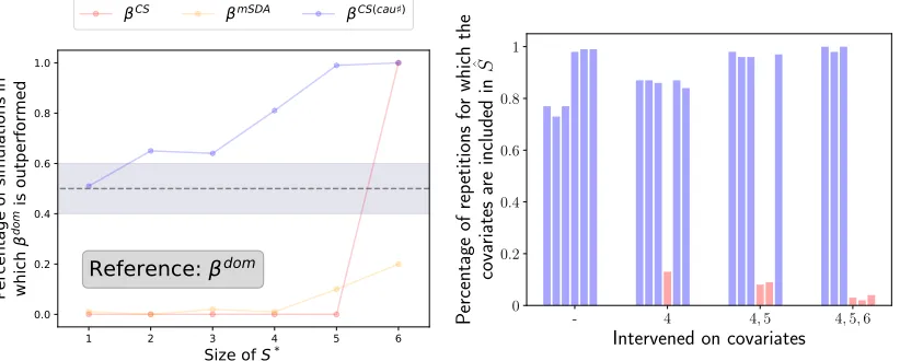
Figure 7: Left: SMTL setting with 6 tasks and 900 examples per task. We plot the percent-age of repetitions (over 100) for which the given methods outperform βdom, as a function of the size of the invariant set S∗. We see that as S∗ becomes larger, more information is transferred from the training tasks, and as such the performance of βCS(cau]) improves. When S∗ is the full set, our method behaves like pooling the data. Right: Covariates se-lected by Algorithm 1 when the training tasks contain interventions only on some of the covariates. The bars represent the percentage of repetitions (out of 100) for which the cor-responding covariates were selected. When there are no interventions in the training tasks, meaning that all the training tasks follow the same distribution, Algorithm 1 systematically selectsall covariates for prediction. When more interventions are performed, however, the corresponding covariates (in red) are excluded in a large number of the repetitions.

thus both methods behave like pooling the data. After a critical value of δ, no subset is accepted, and both algorithms return the subset with the largest p-value.

4.3 Informativeness and subset estimation

The estimation of an invariant subset involves finding a subset for which the residuals have the same distribution across tasks. It is desirable, however, that the selected subset is one which explains the data best. This is ensured by selecting the subset which leads to the smallest error on a validation set. Therefore, some covariates in N may be included in a selected subset if there are no interventions on this covariates in the training tasks. More precisely, if including a covariate does not lead to a statistically measurable difference in the distribution of the residuals between the training tasks, it is advantageous in general to include it in the selected subset since the data is better explained.

0.000 0.015 0.030 0.045 0.060 0.075 0.090

Acceptance level

1.2 1.4 1.6 1.8 2.0 2.2 2.4

MS

E

CS CS(cau) CS(S) CS(Sgreedy)

Figure 8: Logarithm of the empirical squared error in the test task in the DG setting as a function of the acceptance level of the statistical test δ in Algorithm 1. The setup corresponds to t = 3 in Figure 4 (left), also over 100 repetitions. For δ = 0, all subsets are accepted, so the full set of predictors, which minimizes the validation squared error, is selected. Algorithm 1 then returns βCS. As δ increases, no subset is accepted, and Algorithm 1 returns the subset with the largest p-value.

in the selected subset in a large portion of the repetitions, while the other covariates are excluded. This highlights that Algorithm 1 can only exclude covariates whose distribution shifts between training tasks. If being conservative is important for the problem at hand, one can modify Algorithm 1 accordingly, see the end of Section 3.4.

Moreover, in Figure 7 (left) we consider a similar setting, and we compute the perfor-mance against βdom in an SMTL setting as the size of the invariant set increases. We see that as the size of the invariant set increases, the performance of βCS(cau]) improves, since more information is being transferred from the training tasks. When p = 6, traditional covariate shift holds, andβCS(cau]) performs on par with βpool.

4.4 Gene perturbation experiment

We apply our method to gene perturbation data provided by Kemmeren et al. (2014). This data set consists of the m-RNA expression levels of p= 6170 genesX1, . . . , Xp of the

Saccharomyces cerevisiae (yeast). It contains both nobs = 160 observational data points

and nint= 1479 data points from intervention experiments. In each of these interventions,

one known gene (out ofpgenes) is deleted. In the following, we consider two different tasks. The observational sample is drawn from the first task, and the poolednint interventions are drawn from the second task.

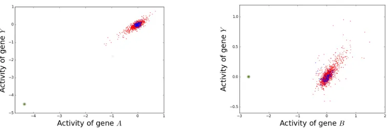
Figure 9: Example of the expression of pairs of genes, where A is causal (left) and B is non-causal (right) of targetY. The blue points are from the observational sample (task 1), the red dots are the interventional sample (task 2), and the green point corresponds to the single interventions in whichA and B are intervened on respectively. On the left, a model learned on the data in red and blue would still perform well on the intervention point, which is not the case on the right.

causal of the activation ofY. For example, Figure 9 shows on the x-axis the activity of two genes (geneA on the left, geneB on the right) such that:

• The expressions of Aand B are strongly correlated with the expression ofY.

• Ais causal ofY (here, we use the definition of a causal effect proposed by Peters et al. (2016)).

• B is non-causal ofY (anticausal or confounded).

In Figure 9 (left), the blue points correspond to the 160 data points from the observational sample, which corresponds to the first task. The red dots are the 1478 data points from the interventional sample, except for the single data point for which A is intervened on, and constitute the second task. The plot on Figure 9 (right) is constructed analogously for B. We can indeed see that in the pooled sample from task 1 and 2,Aand B are both strongly correlated with targetY.

The key difference between both plots are the green points. On Figure 9 (left), the green dot corresponds to the single intervention experiment in which gene A is intervened on. Similarly, the green dot on Figure 9 (right) is the single point in whichB is intervened on. Our goal is to consider the DG setting in which the test task consists on this single intervention point.

For the causal gene A, one expects that a change in the activity of A should translate into a proportional change in the activity ofY. We observe that, in the particular example of the left plot, a linear regression model from A to Y trained only on the pooled data from tasks 1 and 2 (blue and red in Figure 9) would lead to a small prediction error on the intervened point (in green). That is,S∗ ={A}might be a good candidate for a set satisfying Assumptions (A1), (A1’) and (A2). For the non-causal geneB, however, intervening onB

include causal genes as features, but exclude non-causal genes. In these experiments, we aim at testing whether we can exclude non-causal genes such as B automatically.

Setup We address the problem of predicting the activity of a given gene from the remain-ing genes. We are lookremain-ing at the followremain-ing:

• We consider p different problems. In each problem j ∈ {1, . . . , p}, we aim at pre-dicting the activityY =Xj of gene j using (X`)`6=j as features.

• In each problemj∈ {1, . . . , p}, twotraining tasksk∈ {1,2}are available. The data from the first task is the observational sample, and the data from the second task are all the nint interventions (we shall subsequently remove some points for testing, see

below).

The goal is now to apply our method to each of the problems and estimate an invariant subset. Due to the large number of predictors, we first select the 10 top predictor variables using the Lasso and then apply Algorithm 1 to select a set of invariant predictors ˆS, see

βSLassoˆ in Table 2. We denote the indices of the features selected using Lasso by L = (L1, . . . , L10).

The procedure is then evaluated as follows: for each problemj∈ {1, . . . , p}, we first find the genes in (XL1, . . . , XL10) for which an interventional example is available. Note that

this might not hold for all selected genes, since only nint < p interventions are available. We then iterate the following procedure (this is within the context of the same problem): for each gene in (XL1, . . . , XL10) for which an intervention is available,

• we put aside the example corresponding to this intervention from the training data (in the motivation example, this would correspond to the green point).

• we estimate an invariant subset ˆS ⊆L using Algorithm 1 with the remaining obser-vational and interventional data.

• we test all methods on the single intervention point which was put aside.

We expect two different scenarios, as explained in the motivation paragraph above: (1) if the intervened gene is a cause of the target gene, it should still be a good predictor (see Section 2.3); then, it should be beneficial to have this gene included in the set of predictors

ˆ

S. (2) if the intervened gene is anticausal or confounded (we refer to this scenario as

non-causal), the statistical relation to the target gene might change dramatically after the intervention and therefore, one may not want to base the prediction on this gene. In order to see this effect and understand how the different approaches for DG in Table 2 handle the problem, we consider two groups of experiments.

(1) we select the target genesY for which one of the features inLis causal for the activity of Y and for which an intervention experiment is available. 39 problems fall in this causal scenario.

(2) out of the remaining problems we chose target genes with (non-causal) predictors that have been intervened on and — in order to increase the difficulty of the problem — that are strongly correlated with the target gene. We therefore select 269 cases for which a Pearson correlation test (the null hypothesis corresponds to no correlation) outputs a p-value equal to zero.

βCS(cau)

βCS( ˆSLasso) _βCS _βmean

βDICA

0 2 4 6 8 10 12 14

Squared

error

on

test

genes

(causal)

βCS(cau)

βCS( ˆSLasso) _βCS _βmean

βDICA

0.0 0.2 0.4 0.6 0.8 1.0

Squared

error

on

test

genes

(non-causal)

0 10 20 30 40 50

Multiplicative factorτ 0

20 40 60 80 100 120 140 160

Number

of

test

genes

(non-causal)

βCS

βCS( ˆSLasso)

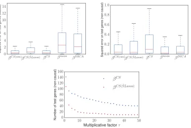
Figure 10: In the causal problems (top left), interventions are performed on causal genes. As expected, the input genes continue to be good predictors, and βCS works well. In the non-causal problems (top right), one of the inputs is intervened upon and becomes a poor predictor, impairing the performance of βCS. The mean predictor βmean uses none of the predictors, and therefore works comparatively well in this scenario. Our proposed estimator

βCS( ˆS)provides reasonable estimates in both the causal and non-causal settings, while other methods only perform well in one of the scenarios. βDICA performs similarly to βmean in both scenarios, and is therefore outperformed by other methods in the causal problems (note that βDICA uses all available features). Bottom: in the non-causal scenario (2), we plot the number of test genes for which the squared error forβCS is larger thanτ times the squared error for βCS( ˆS), and vice-versa, where τ is plotted on the x-axis. This plot shows the number of genes for which one of the method does significantly worse than the other. By this measure, βCS( ˆSLasso) outperformsβCS for all values ofτ.

scenario. As expected, pooling does well in this setting. Figure 10 (bottom) shows that in the non-causal problems (2), prediction using an invariant subset leads to less severe mistakes on test genes compared to pooling the tasks.

5. Conclusions and further directions

We propose a method for transfer learning that is motivated by causal modeling and exploits a set of invariant predictors. If the underlying causal structure is known and the tasks correspond to interventions on variables other than the target variable, the causal parents of the target variable constitute such a set of invariant predictors. We prove that predicting using an invariant set is optimal in an adversarial setting in DG. If the invariant structure is not known, we propose an algorithm that automatically detects an invariant subset, while also focusing on good prediction. In practice, we see that our algorithm successfully finds a set of predictors leading to invariant conditionals when enough training tasks are available. Our method can incorporate additional data from the test task (MTL) and yields good performance on synthetic data. Although an invariant set may not always exist, our experiment on real data indicates that exploiting invariance leads to methods which are robust against transfer.

As we saw in the DG and MTL experiments,βSˆdoes not always performs as well asβcau, which uses the ground truth. We believe that alternative methods for estimating the set ˆS

may close this gap. Furthermore, extending our framework to nonlinearities seems straight-forward and may prove to be useful in many applications. For instance, we provide a general, nonlinear version of Theorem 1 in Appendix A. Moreover, Algorithms 1 and 2 are presented in a linear setting. However, the extension to a nonlinear framework is straightforward. In particular, the linear regression can be replaced by a nonlinear regression method. We expect that there may be feature maps leading to invariant conditionals that are different from a subset.

We expect our method to be favorable in (adversarial-like) situations with strong dif-ferences between the tasks, such as the gene experiment in Section 4.4. We also evaluated our method on the School dataset (Bakker and Heskes, 2003), but found that we do not do better than pooling the data (we also do not do worse, the results are not shown). We believe this may be due to the fact that the difference between the tasks in this dataset are not too large.