Recent Updates in Two Competitive Algorithms
for Model Reduction of Large-Scale Dynamical
Systems
Mohammed Nizam Uddin1*, Mohammad Monir Uddin2, Muhammad Hanif1
1
Department of Applied Mathematics, Noakhali Science and Technology University, Sonapur, Noakhali-3814, Bangladesh
2
Department of Mathematics and Physics, North South University, Dhaka-1229, Bangladesh
Abstract — The modern approach, to explore scientific ideas to convince others of their validations, is through computer simulations. In simulation, one needs to convert a physical model into a mathematical model. Often also in real-life applications the mathematical models are represented by linear time-invariant (LTI) continuous-time systems. A large system leads to additional memory requirements and enormous computational efforts. Therefore,reducing the size of the system is an indispensable task for fast simulations. Various techniques are proposed in the literature to reduce the size of the large-scale LTI continuous-time systems. Among those, the Gramian based method Balanced truncation (BT) and interpolatoryprojection based method Iterative rational Krylov algorithm (IRKA) are most commonly used techniques. This article shows the comparisons between the BT andIRKA using their recent developments.
Index Terms — LTI continuous-time system, model reduction,balanced truncation, iterative rational Krylov algorithm.
I. INTRODUCTION
In this article we describe generalized LTI continuous-time systems of the form:
𝐸𝑥(𝑡) = 𝐴𝑥(𝑡) + 𝐵𝑢(𝑡);(1)
𝑦(𝑡) = 𝐶𝑥(𝑡) + 𝐷𝑢(𝑡);
where the vector x(t) ∈Rnis the state vector, u(t) ∈Rpis the input vector and y(t) 2 Rmis the output vector and E. , BC
and D are all matrices with appropriatedimensions. If p = m = 1, the system is referred to as a single-inputsingle-output (SISO) system, otherwise it is called a multiinput multi-single-inputsingle-output (MIMO) system. In the MIMO case, we assume that the number of inputs andoutputs are much less than the number of states, i.e., p; m << n. Thecorresponding transfer function of this system is defined by
G(s) = C(sE - A)-1B + D, (2)
where s ∈C. In real-life applications such mathematical models arise in different disciplines of science and engineering. See, e.g., [1], [2] for some motivating examples. In general, such systems are generated by finite element or finite difference methods (cite here). If the grid resolution becomes very fine, because many details must be resolved, the systems become very large. Moreover they are sparse, i.e., most of the elements in the matrices of the system are zero, which are not stored. A high dimensional system will always be complex, requiring a great deal of memory, thereby hindering computational performance significantly in simulation. Sometimes the systems are too large to store due to memory restrictions. Therefore, we seek to reduce the complexity of the model by applying model order reduction (MOR), i.e., we want to approximate the system (1) by the lower dimensional model:
𝐸 𝑥 𝑡 = 𝐴 𝑥 𝑡 + 𝐵 𝑢 (𝑡), 𝑦 (𝑡) = 𝐶 𝑥 (𝑡) + 𝐷 𝑢(𝑡),(3)
where 𝐸 , 𝐴 ∈ Rlxl‘ב and B ∈RlxpC∈ RmxlandD ∶=D The quality of the reduced order model (ROM) relies on the difference of the two outputs y and y^ which can also be measured by
||𝐺 . − 𝐺 . ||, (4)
where 𝐺 (𝑠) = 𝐶 (𝑠𝐸 − 𝐴 )−1𝐵, 𝑠 ∈ 𝐶 is the transfer functions of (3). Note that k:kdenotes a suitable norm e.g., the H1 or H2 norms (see [1]). For motivations, applications, restrictions, and techniques of MOR see, e.g., [1], [2].
Gramian based methods and momentmatching based methods. Recently, two prominent methods, namely the balanced truncation (BT) and the iterative rational Krylov algorithm (IRKA) based interpolatory projection method are frequently used for the model reduction of large-scale dynamical systems. Both of them have merits and demerits. Balanced truncation preserve stability of the system and it has an a-priori error bound. However, in this method one has to solve two Lyapunov equations which is computationally expensive. On the other hand, the recentlydeveloped,interpolatory method via IRKA is attractive to the model reduction community since it is computationally efficient. It requires only matrix - vector products or linear solves. Unfortunately, this prominent method has neither an a-priori error bound nor guaranteed stability preservation. In this article we show the comparisons of these two prominent techniques i.e., the BT and IRKA using their recent updates . II. BALANCED TRUNCATION (BT) A good motivation of balanced truncation can be found in [1]. The fundamental idea of balanced truncation is to truncate the less-important states from a system. A less-important state is a state that is difficult to control and observe. Those states essentially correspond to the smallest Hankel Singular values (HSVs) of the system. In reality, the states which are difficult to control may not be difficult to observe and vice versa. This implicates if we eliminate the states that are hard to be controlled directly from the original system, then we may also eliminate some states that are easy to observe.However,in an application, the easily observable states are essential to be preserved. The same contradiction might appear for those states that are difficult to be observed but easily controlled. This problem can be resolved by transforming the system into a balanced form. In a balanced, system the degree of controllability and the degree of observability of each state are the same. A balanced system can also be defined as follows.
Definition II.1. A stable and minimal LTI system is called balanced if the controllability Gramian and the observability Gramian of the system are equal and diagonal. The diagonal elements are the system’s HSVs.
The system’s controllability Gramin (P) and observability Gramain (Q) are the solutions of the following two Lyapunov equations
APET+ EPAT= -BBT(5) AT QE + ETQA = -CTC(6)
respectively. Equation (5) and (6) are respectively, known as continuous-time controllability and observability Lyapunov equations. In a balanced system the relation
P = Q = diag (σ1, σ2,… ,σn)
holds true. A system can be balanced via the balancing transformation.
Definition II.2.A state space transformation T is called balancing transformation if it causes
TP T*=T-*QT-1= ∑1
∑2
, (7)
where P and Q are the controllability and observ -ability Gramians, Σ1 = diag (σ1,...., σr), Σ2=diag (σr+1,…, σn), and 𝜎𝑖 𝑖=1 𝑛 are the system’s HSVs.
Under the balancing transformations, according to theGramians in (7), the state space realization is transformed into (E, A, B, C, D) →(TET-1, TAT-1, TB, CT-1, D )= 𝐸𝐸11 𝐸12
21 𝐸22 ,
𝐴11 𝐴12
𝐴21 𝐴22 , 𝐵1
𝐵2 , 𝐶1 𝐶2 , 𝐷 .
Now picking up the block matrices E11, A11, B1, C1 one can form the ROM (3), where (𝐸 , 𝐴 , 𝐵 , 𝐶 ) = (E11, A11, B1,
C1).From the above discussion we can conclude that in the balancing based model reduction one must first compute
the balancing transformation (T) to convert the system into a balanced form. Then the truncation is performed on the balanced system. For a large-scale system, balancing the whole system before truncation is infeasible. Hence, for such systems, usually the balancing and truncation are carried out simultaneously, by using the so-called balancing
and truncating transformations. The author of [1] reviews several approaches to compute the balancing and
truncating transformations among which we will focus on the square-root method (SRM), originally defined in [3]. To perform this method, we compute the Gramian factors Rcand Lc, such that P = RcRcT; Q = LcLTc Then the
balancing transformation can be formed using the SVD
𝑅𝑐𝑇 𝐸𝐿
𝑐 = 𝑈𝛴𝑉𝑇 = 𝑈1 𝑈2 ∑1 ∑ 2
𝑉1
𝑇
Algorithm 1: LR-SRM.
Input :E,A,B,C,D
Output:𝐸 , 𝐴 , 𝐵 , 𝐶 , 𝐷 ≔ 𝐷
1 Compute R and L as defined in (9) by solving the Lyapunov equations (5) and (6).
2 Compute SVD
RTEL = UΣV T= 𝑈1 𝑈2 ∑1 ∑ 2
𝑉1
𝑇
𝑉2𝑇
3 Construct 𝑉 ≔ 𝐿𝑉1Σ1−
1 2
, W ≔RU1Σ1
− 12
4 Form
𝐸 = 𝑊𝑇𝐸𝑉, 𝐴 = 𝑊𝑇𝐴𝑉, 𝐵 = 𝑊𝑇𝐵, 𝐶 = 𝐶𝑉
and defining
𝑉 ≔ 𝐿𝐶𝑉1Σ1 − 12
, 𝑊 ≔ 𝑅𝑐𝑈1Σ1 − 12
, (8)
where 𝑈1and 𝑉1are composed of the leading k columns of U and V , respectively, Σ1 is the first k × k block of the matrix Σ = diag (σ1, σ2,…, σk,…, σn). Finally, by applying the balancing transformations to the system (1), one can
derive the ROM (3).TheGramian factors Rcand Lcare obtained by usingthe Cholesky decompositions of the GramiansP and Q. The Gramians can be computed by solving the corresponding Lyapunov equations (5) and (6). There exist direct solvers [4] as well as iterative solvers [5] to compute P and Q from (5-6).All these methods are applicable for a small dense systems. If the number of inputs and outputs are much smaller than the dimension of the system, then the GramiansP and Q can usually be approximated by low-rank factors, i.e,
P ≈ RRTand Q ≈ LLT(9)
where R and L are thin rectangular matrices. Therefore, instead of computing the full Gramian factors, one can compute low-rank factors of the Gramians. During the last few decades, several iterative methods were proposed, e.g., lowrank Cholesky factor - alternating direction implicit (LRCFADI) iterations [6], cyclic low-rank Smith methods [7], projection methods [8], and sign function methods [9]. Although most of the methods are shown to be applicable for large scale dynamical systems, the LRCF-ADI iteration is more attractive in the context of Gramian based model reduction for large sparse systems with few inputs and outputs. A motivation of this prominent method can be found in [10]. Readers are referred to [11, Chapter 2] to see the updated algorithm and implementing details of LRCF-ADI method.
Using the low-rank Gramian factors R and L, the squareroot method is summarized in Algorithm 1. Note that weuse [11,Algorithm 5] to compute the R and L. The reducedsystems obtained by this algorithm satisfies [1] the global error bound
||𝐺 − 𝐺 ||𝐻∞≤ 2 ∑𝑛 𝜎𝑖
𝑖=𝑘+1 (10)
where 𝐺is the transfer function of the reduced model. Therelation (10) is an a-priori error bound. Thus, for a given errorbound (tolerance) one can use it to fix the required dimensionof the reduced system.
III. ITERATIVE RATIONAL KRYLOV ALGORITHM (IRKA)
Interpolatory projection methods seek a ROM (3) by constructing the matrices V and W in such way that the reducedtransferfunction defined in (4) interpolates the original transferfunction (2) at a predefined set of interpolation points. Thatmeans to find𝐺 (s) such that
G(αi) = 𝐺(αi);
where αi∈C are the interpolation points. Often, in additionto the above conditions, we are interested in matching
more
quantities, that is G(j)( αi) =𝐺 (j)( αi);
C[(αi E –A)-1E]j(αi E - A)-1B:= (12) 𝐶 [(αi𝐸 –𝐴 )-1𝐸 ]j(αi𝐸 - 𝐴 )-1𝐵 ,
for j = 0,1,…, q; where C[(αi E –A)-1E]j(αi E - A)-1Bis called the j-th moment of G(s) at αi, and 𝐺 (j)(αi) represents the
j-thderivative of G(s) evaluated at σI. Note that forj = 0, these conditions reduce to (11). In this paper, we restrict
ourselves to simpleHermite interpolation (Cite here), wherej = 0 and j = 1. In the following, we discuss how a ROM can be generated by computingfirst the appropriate projection so that a reduced interpolating approximation is guaranteed. The concept of projection forinterpolatory model reduction was first discussed in [12], and later, Grimme in [13] modified the approach by utilizing therational Krylov method [?]. Since Krylov based methods can achieve moments matching without explicitly computing themoments (explicit computationof moments is known to be ill-conditioned [14]), they areextremely useful for model reduction of large scale systems.
The following Lemma suggests a choice of V and W thatensure Hermite interpolation with the use of a rational Krylovsubspace.
Lemma III.1([15]). Let us consider two sets of distinctinterpolation points, { 𝛼𝑖}𝑖=1𝑟 ⊂Cand { 𝛽𝑖}𝑖=1𝑟 ⊂C,whichare closed under conjugation (i.e., the points are either realor appear in conjugate pairs). Suppose V and W satisfy
Range (V ) = span {(α1E - A)-1B,…,(αrE- A)-1B}, (13a)
Range (W) = span {(β1ET-AT)-1CT,…,(βrET- AT)-1CT }, (13b)
Then V and W can be chosen real and 𝐺 (s) = 𝐶 (s𝐸 –𝐴 )-1𝑐 where 𝐸 ,𝐴 ,𝐵 and 𝐶 are defined in (3), satisfies theinterpolation conditions
G(αi) =𝐺 (αi); G(βi) = 𝐺 (βi); and 𝐺’(αi) = 𝐺 ′ (αi) when αi= βi;
for i= 1,…, r.The subspace in (13a), that is, the span of the column vectors (αiE- A)-1B for i= 1,…, r, can be
considered as the union of shifted rational Krylov subspaces. For a given shift frequency α ∈C, the rational KrylovsubspaceKq((αE - A)-1; (αE - A)-1B) is defined as
Kq((αE - A)-1; (αE - A)-1B) :=span (αE - A)-1B,…,(αE - A)-qB.
If q = 1 for each ( αi,i= 1,…, r, then the union of suchshifted rational Krylov subspaces is equivalent to the subspace
in (13a). Analogously, the subspace in (13b) can also be defined as the union of shifted rational Krylov subspaces given above. Tosummarize, rational Krylov based model reduction requires a suitable choice of interpolation points, the construction of V and W as in Lemma III.1, and the use of Petrov-Galerkin conditions (cite here).The quality of the reduced model is highly dependent on the choice of interpolation points and therefore various techniques [12] have been developed for the selection of interpolation points. Recently in [15], the issue of selecting a good choice of interpolation points is linked to the problem of H2-optimal model reduction.
Definition III.2. A ROM (3) is called H2 optimal if it satisfies
𝐺
𝐻2=min||𝐺 − 𝐺 ||𝐻∞. (14)
dim (𝐺 )=r
Now a days IRKA becomes of of the best choice in MOR using Krylov subspace approaches [15]. Upon convergence, itidentifies a choice of interpolation points that guarantees the H2-optimality conditions for the reduced
system. Starting from an initial set of interpolation points, the IRKA iteration updates the interpolation points until they converge to a fixed value. A complete procedure of IRKA for a SISO system is given in [15, Algorithm 4.1].For model reduction of MIMO dynamical systems, rationaltangential interpolation has been developed by Gallivan et. al. [16]. The problem of rational tangentialinterpolation is to construct V and W such that the reduced transfer function𝐺 (s) tangentiallyinterpolates the original transfer functionG(s) at a predefined set of interpolation points and some fixedtangent directions. That is
where bi ∈Cmand ci∈Cpare the right and left tangentialdirections, respectively, and both correspond to the
interpolation points αi. With these quantities, the rational tangential interpolation can be achieved. The IRKA based interpolatoryprojection methods for MIMO systems have been discussed in [15], where the algorithm updates interpolation points as well as tangential directions until the reduced system satisfies the necessary condition for H2
optimality. We have summarized a complete procedure for a MIMO system in Algorithm 2.
IV. NUMERICAL RESULTS
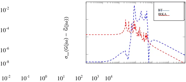
This section discusses the numerical results to show thecomparisons between the BT and IRKA based model reduction methods. We consider a model example; the International Space Station model (ISSM). The details of the model can be found in [17]. The dimension of the original model is 270 and the number of inputs-outputs are 3. For each model we compute different dimensional reduced models via projecting the systems onto the eigen-space of Gramians.Applying Algorithm 1 and 2 we form exemplary reduced order models of dimension 50. Figure 1 shows the frequency responses (largest singular value of G(𝜔) of full and the 50dimensional reduced order models obtained by BT and IRKA in frequency domain over range of 10-2to104. The absolute error between the frequency responses of full and reduced
Algorithm 2: IRKA for MIMO systems.
Input :E,A,B,C,D
Output: 𝐸 , 𝐴, 𝐵 , 𝐶 , 𝐷 ∶= 𝐷.
1 Make an initial selection of 𝛼𝑖 𝑖=1𝑟 and 𝑏𝑖 𝑖=1𝑟
𝑐𝑖 𝑖=1𝑟
2 V = [(α1E - A)-1Bb1,…, (αrE - A)-1Bbr]
3W =[ (α1ET - AT)-1CT c1; · · · ; (αrET – A)-1CT cr.]
4 while (not converged) do
5 𝐸 = WT EV , 𝐴 = WT AV , 𝐴 = WT B, 𝐶 = CV .
6 Compute A𝑧 i= 𝜆 i E𝑧 iand 𝑦𝑖∗𝐴 = 𝜆 𝑖𝑦𝑖∗𝐸 .
7 𝛼𝑖 ← 𝜆𝑖, 𝑏𝑖∗← 𝑦𝑖∗𝐵 and 𝑐𝑖 ← 𝐶 𝑧𝑖, for i= 1,…, r.
8 V = [(α1E - A)-1Bb1; · · · ; (αrE - A-1Bbr],
W = (α1ET - AT)-1CT c1,…, (αrET - AT)- 1Ccr.
9 i=i+ 1
10 𝐸 = 𝑊𝑇𝐸𝑉, 𝐴 = 𝑊𝑇𝐴𝑉, 𝐵 = 𝑊𝑇𝐵𝑎𝑛𝑑𝐶 = 𝐶𝑉.
10-2
10-4
10-6
10-2 10-1 100 101 102 103 104
Fig. 1: Sigma plot (maximum singular values) of full andreducedorder models.
models are shown in Figure 2. In both the cases the computed errors are satisfactory. This figure deficits that in the lower frequencies the performances of the BT method is better than the IRKA. On the other hand in the higher frequencies the result is vice versa.
full model BT IRKA
𝜎𝑚
𝑎
𝑥
(𝐺
(𝑗
𝜔
10-2
10-4
10-6 10-8
10-2 10-1 100 101 102 103 104
Fig. 2: Absolute error in the sigma plot of full and reducedorder models.
V. CONCLUSIONS
In this article we have discussed two prominent methods,such as balanced truncation and IRKA for model reductionof large-scale LTI continuous-time systems. The advantages and disadvantages of both methods have been discussed elaborately. For theboth methods we havepresented the updated algorithms of the MIMO systems. The comparisons are also shown by using numerical results.
REFERENCES
[1] A. Antoulas, Approximation of Large-Scale DynamicalSystems, ser.Advances in Design and Control. Philadelphia, PA: SIAM
Publications,2005, vol. 6.
[2] P. Benner, V. Mehrmann, and D. C. Sorensen, Dimension Reduction ofLarge-Scale Systems, ser. Lect. Notes Comput. Sci. EngSpringer-
Verlag, Berlin/Heidelberg, Germany, 2005, vol. 45
[3] M. S. Tombs and I. Postlethwaite, “Truncated balanced realization of a stable non-minimal state-space system,” Internat. J. Control, vol.
46,no. 4, pp. 1319–1330, 1987.
[4] R. H. Bartels and G. W. Stewart, “Solution of the matrix equation AX+XB = C: Algorithm 432,” Comm. ACM, vol. 15, pp. 820–826,
1972.
[5] P. Benner and E. S. Quintana-Ort´ı, “Solving stable generalized Lyapunovequations with the matrix sign function,” Numer. Algorithms,
vol. 20,no. 1, pp. 75–100, 1999.
[6] J.-R. Li and J. White, “Low rank solution of Lyapunov equations,” SIAMJ. Matrix Anal. Appl., vol. 24, no. 1, pp. 260–280, 2002.
[7] T. Penzl, “A cyclic low rank Smith method for large sparse Lyapunovequations,” SIAM J. Sci. Comput., vol. 21, no. 4, pp. 1401–1418,
2000.
[8] Y. Saad, “Numerical solution of large Lyapunov equation,” in SignalProcessing, Scattering, Operator Theory and Numerical Methods,
M. A.Kaashoek, J. H. van Schuppen, and A. C. M. Ran, Eds. Birkhauser, ¨1990, pp. 503–511.
[9] U. Baur, “Control-Oriented Model Reduction for Parabolic Systems,” Ph.D. Thesis, TechnischeUniversitat Berlin, Berlin, Jan. 2008,
iSBN 978-3639074178 Vdm Verlag Dr. Muller, available from http://www.nbn-resolving.de/urn:nbn:de:kobv:83-opus-17608.
[10] P. Benner and J. Saak, “Numerical solution of large and sparse continuous time algebraic matrix Riccati and Lyapunov equations: a state
ofthe art survey,” GAMM Mitteilungen, vol. 36, no. 1, pp. 32–52, August2013.
[11] M. M. Uddin, “Computational methods for model reduction of large-scale sparse structured descriptor systems,” Ph.D.
Thesis,Otto-von-Guericke-Universitat, Magdeburg, Germany, 2015. [Online]. Available: http://nbn-resolving.de/urn:nbn:de:gbv:ma9:16535
[12] D. C. Villemagne and R. E. Skelton, “Model reduction using a projectionformulation,” Internat. J. Control, vol. 46, pp. 2141–2169, 1987.
[13] E. J. Grimme, “Krylov projection methods for model reduction,” Ph.D.Thesis, Univ. of Illinois at Urbana-Champaign, USA, 1997.
[14] P. Feldmann and R. W. Freund, “Efficient linear circuit analysis by Pade´ approximation via the Lanczos process,” IEEE Trans.
Comput.-AidedDesign Integr. Circuits Syst., vol. 14, pp. 639–649, 1995.
[15] S. Gugercin, A. C. Antoulas, and C. A. Beattie, “H2 model reductionfor large-scale dynamical systems,” SIAM J. Matrix Anal. Appl., vol.
30,no. 2, pp. 609–638, 2008.
[16] K. Gallivan, A. Vandendorpe, and P. Van Dooren, “Model reductionof MIMO systems via tangential interpolation,” SIAM J. Matrix
Anal.Appl., vol. 26, no. 2, pp. 328–349, 2004.
[17] Y. Chahlaoui and P. Van Dooren, “A collection of benchmark examples for model reduction of linear time invariant dynamical
systems,”University of Manchester, SLICOT Working Note 2002–2, Feb. 2002,ava
BT IRKA
σmax
(G
jω
−
G
(j
ω