D. Bresch, V. Calvez, E. Grenier, P. Vigneaux & J.-F. Gerbeau, Editors
A RAINBOW INVERSE PROBLEM
A. Blasselle
1, V. Calvez
2and A. Moussa
3Abstract. We consider the radiative transfer equation (RTE) with reflection in a three-dimensional domain, infinite in two dimensions, and prove an existence result. Then, we study the inverse problem of retrieving the optical parameters from boundary measurements, with help of existing results by Choulli and Stefanov. This theoretical analysis is the framework of an attempt to model the color of the skin. For this purpose, a code has been developed to solve the RTE and to study the sensitivity of the measurements made by biophysicists with respect to the physiological parameters responsible for the optical properties of this complex, multi-layered material.
R´esum´e. On ´etudie l’´equation du transfert radiatif (ETR) dans un domaine tridimensionnel infini dans deux directions, et on prouve un r´esultat d’existence. On s’int´eresse ensuite `a la reconstruction des param`etres optiques `a partir de mesures faites au bord, en s’appuyant sur des r´esultats de Choulli et Stefanov. Cette analyse sert de cadre th´eorique `a un travail de mod´elisation de la couleur de la peau. Dans cette perspective, un code `a ´et´e d´evelopp´e pour r´esoudre l’ETR et ´etudier la sensibilit´e des mesures effectu´ees par les biophysiciens par rapport aux param`etres physiologiques tenus pour responsables des propri´et´es optiques de ce complexe mat´eriau multicouche.
Introduction
Skin is a complex multi-layered media and the most important organ of our body in terms of weight, surface and functionalities. For many years, physicists have tried to understand what physiological components or properties are responsible for its color. The color of an object is defined by a unidimensional curve called the reflectance spectrum, which is the relative energy given back by the object for each wavelength of the visible range, when it is enlighted with a white spot. Physicists have developed a lot of models to link the physiological components of the skin (like, for example, the blood concentration or the diameter of the melanosomes) to its optical properties. Physicists have simulated, by many ways, how light travels into the skin. What has not been theoretically investigated yet, even if very well studied by Magnain, Elias and Frigerio in [2], is the inverse problem of retrieving the physiological parameters from measurements made at the surface of the skin. Before studying the inverse problem, we tried to simulate the direct one, and developed a small Matlab code to do so. This code is proved to be quite satisfying for this purpose, hence we used it to make a sensitivity study of the reflectance curves with respect to the physiological parameters. We went on with the theoretical study of this inverse problem, in a very simplified framework and based on the existing work of Choulli and Stefanov [5]. The paper is organized in the reverse order: theoretical study, then numerical results.
1
Laboratoire Jacques-Louis Lions, 175 rue du Chevaleret, 75013 Paris, e-mail:[email protected]
2
UMPA, ENS Lyon, 46, all´ee d’Italie 69364 Lyon Cedex 07, e-mail: [email protected]
3
CMLA, Cachan, 61 Avenue du Pr´esident Wilson, 94235 Cachan Cedex, e-mail:[email protected]
©EDP Sciences, SMAI 2010
1.
Modeling
1.1.
The radiative transfer equation
When light enters an object X, the photons propagate in straight line, unless they are absorbed by the material or scattered (and possibly deviated) by various entities. One classical way to describe the light intensity is the use of aprobability density function (p.d.f.): f, that depends on the positionxand the velocityv of the photon.
The set of all possible directions,V is all or part of the sphereS2. The physical interaction with the material
is described by:
• the absorption coefficientµa (given inm−1), which is the number of absorption events per unit length and depend on the position and the direction: µa =µa(x, v),
• the scattering coefficientµs=µs(x, v) (also inm−1), the same quantity for the scattering,
• the kernelp=p(x, v, w) which is a probability density with respect tov. It denotes the probability for a photon arriving with the directionw, to get a new directionv after having hit a scatterring center. If the scattering centers are distant enough from one another (compared to the wavelength), the radiative transfer equation (RTE) describes properly the behaviour of the light intensity:
v· ∇xf+ (µa(x, v) +µs(x, v))f(x, v) =
Z
V
µs(x, w)p(x, v, w)f(x, w) dw, inX×V. (1)
1.2.
Geometry and boundary conditions
The equation (1) has been written with no internal source of light, and has to be complemented by boundary conditions to model the enlightment of the object. The typical experiment we are interested in is the following: the skin is enlighted from its top, on a large surface, and its color is registered on the same zone. At this scale, the two others dimensions can be considered as infinite. Indeed, the thickness of the whole skin is of the order of 10−3m, whereas the skin is much more extended over our body. Hence, we will model our skin sample as a
box infinite in the two planar directions.
When travelling into the skin, the light will encounter several interfaces, one of them being the epidermis-dermis junction. Part of the light will get through it, but the remaining amount will be reflected. Hence, our boundary conditions will be:
• a source functionf− modeling the enlightment on the top,
• reflection of part of the light at each interface encountered.
2.
Theoretical inverse problem
Choulli and Stefanov have already proved in [5] that the parameters can be uniquely determined by surface measurements, under the following assumptions, in the case where the RTE (1) is complemented with Dirichlet boundary conditions. We will conduct the same study with mixed boundary conditions by adding a reflection operator. Before getting into the inverse problem, we have to show existence of the light intensity for the direct problem.
2.1.
Notations and functional framework
We focus in this study on a single layer, so that the first interface encountered is the bottom of the sample. Hence, the position and velocity spaces are:
Source
Scattering event
Reflexion at the bottom Skin surface
~ e1
~ e2
~ e3
Figure 1. Model of the skin
We consider a system of axis onX whose first direction is normal to the plane of the skin, as illustrated in Figure 1.2. All points belonging to the boundary ofX (that is∂X ={0} ×R2∪ {L} ×R2) are denoted with a
prime symbol: x′,y′ and so forth. Forx′ ∈∂X, we denote byn(x′) the outward-pointing normal vector. The following sets will be widely used:
Γ±={ξ= (x′, v)∈∂X×V /±v·n(x′)>0},
with the measure dξ=|v.e1|dx′dv. We define the first time of exit by outward (resp. downward) directions:
τ±(x, v) = min{t≥0|x±tv∈∂X}, τ(x, v) =τ−(x, v) +τ+(x, v).
We also introduce the absorption coefficient, and the full scattering kernel:
σa(x, v) =µa(x, v) +µs(x, v),
k(x, v, w) =µs(x, w)p(x, v, w).
The enlightment is modeled by f− ∈ L1(Γ−,dξ). The coefficients are assumed to satisfy the following regularity properties [6]:
(i) 0≤µs∈L∞(X×V) and 0< ν≤µa∈L∞(X×V), (ii) 0≤k(x, v, .)∈L1(V) for a.e. (x, v)∈X×V.
The problem will be studied in the following functional space:
W ={f ∈L1(X×V) s.t. v· ∇f ∈L1(X×V)}. (3)
Thanks to Cessenat [3, 4], we know that iff ∈W, its traces on Γ± exist and we give the theorem in the case of L1 spaces:
We denote classically the albedo operator as follows:
Af− =f|Γ+,
where f(x, v) satisfies (1) with the boundary conditionf =f− on Γ−. The Boundary Value Problem admits a unique solution in W if f− ∈ L1(Γ−, dξ) [6]. Also the albedo operator A : L1(Γ−, dξ˜) → L1(Γ+, dξ˜) is a bounded operator, where the boundary measuredξ has been replaced bydξ˜= min{τ(x, v), K}|v·e1|dx′dv for
some positive numberK [5].
2.2.
The direct reflection problem
We define a general reflection operatorR: L1(Γ+,dξ)→L1(Γ−,dξ) by:
Rϕ=
Z
w.n(x′)>0
m(x′, v, w)ϕ(x′, w) dw, (4)
where m(x′, v, w) is a boundary transition kernel such thatR satisfies the following assumption: there exists 0≤α <1 such that,
∀ϕ∈L1(Γ+, dξ) kRϕkL1(Γ−,dξ)≤αkϕkL1(Γ+,dξ). (5)
If, under our geometrical framework (plane interfaces), we assume that the skin satisfies Snell-Descartes reflection laws at its interfaces (like in our numerical implementation), some grazing rays may be trapped in the material because of the values of the optical indices if we do not remove the planar directionsv (such that
v.e1= 0). Hence, the latter assumption is not satisfied for the corresponding reflection operator. The equation
(5) expresses that every direction is uniformly partially absorbed (or refracted). In our code, we removed the grazing directions with the angular discretization.
The direct problem we are interested in writes:
v· ∇xf(x, v) +σa(x, v)f(x, v) =
Z
V
k(x, v, w)f(x, w) dw inX×V
f|Γ− =f−+Rf|Γ− on Γ−
(6)
Theorem 2.2. Suppose that f− ∈L1(Γ−,dξ), the reflection operator Rverifies (5) and assumptions (i)and (ii)hold true. Then the problem (6)has a solution f inW.
Proof. We define the operatorT : L1(Γ−,dξ)→L1(Γ−,dξ):
Tg=R ◦ Ag. (7)
We know that this system has a unique solution inW. We have that T is a contraction operator. Assume first thatg andf are nonnegative functions. If we integrate (1) onX×V and use Green formula, we get:
Z
Γ+
v·n(x′)f|Γ+(x′, v) dx′dv+ Z
Γ−
v·n(x′)g(x′, v) dx′dv+
Z
X×V
σa(x, v)f(x, v)dxdv
=
Z
X×V
Z
V
k(x, v, w)f(x, w)dxdvdw
=
Z
X×V
µs(x, w)f(x, w)dxdw.
Therefore we have: Z
Γ+
f|Γ+dξ− Z
Γ−
gdξ=−
Z
X×V
For a function whose sign is unknown, we begin by multiplying (1) by sgn(f)(x, v) and then we integrate by parts. Using the fact that ∇|f| = sgn(f)∇f, and sgn(f)f =|f| we obtain the exact same conclusion for functions having no specific sign, namely that:
kfkL1(Γ+,dξ)≤ kgkL1(Γ−,dξ).
The assumption (5) directly ensures thatT is a contraction operator. Denoting byIthe identity of L1(Γ−, dξ), we know that I− T is invertible. Thereby the solution of (6) satisfies
(I− T)f =f− on Γ−. (8)
2.3.
The inverse problem without reflection
We assume in this Section that the absorption coefficientσa does not depend on the velocity v. In [5], the authors prove that under suitable assumptions, the albedo operator A : f− →f|Γ+ determines uniquely the
coefficient σa(x). In addition, when the space dimension is equal or larger than 3, the albedo operator also characterizes the scattering kernelk(x, v, w).
We briefly sketch their arguments below. The main idea is to decompose the albedo operator into three parts: the solution to (1) with the boundary condition f− = δΓ−(x′ −x′
0)δV(v−v0) is given by f(x, v) = f1(x, v) +f2(x, v) +f3(x, v), where f1 is the contribution of an incoming laser subject to absorption only. It
verifies:
v· ∇f1(x, v) +σa(x)f1(x, v) = 0, (9)
and the solution is explicitely given by:
f1(x, v) =|n(x′0)·v0|
Z τ+(x,v)
0
exp −
Z τ−(x,v)
0
σa(x−pv) dp
!
δ(x−x′
0−tv)δ(v−v0) dt. (10)
The second contribution f2 results from trace of this laser (a single line parametrized by x′0+tv0) which is
scattered and absorbed. It satisfies:
v· ∇xf2(x, v) +σa(x)f2(x, v) =α(x, v0)k(x, v, v0)δ(x−τ−(x, v0)v0), (11)
and the solution is explicitely given by:
f2(x, v) =|n(x′0)·v0|
Z τ−(x,v)
0
Z τ+(x,v)
0
exp
−
Z s
0
σa(x−pv) dp
×exp −
Z τ−(x−sv,v0) 0
σa(x−sv−pv0) dp
!
k(x−sv, v0, v)δ(x−x′0−sv−tv0) dtds. (12)
The reminderf3has no explicit formulation. However it is proven in [5] that it is a function. Namely, it satisfies
the following estimate:
(min{τ, K})−1|n(x′
0)·v0|−1f3(x, v)∈L1(X ×V) uniformly in (x′0, v0). (13)
Let us sketch the arguments of [5] in our context (see also [1] for a comprehensive review). We restrict to
x′
0= 0 for the sake of clarity. At first glance we look for a solution of the form
whereg(x, v) contains lower order distribution terms (namely either the support of the singular parts is of lower dimension, or they are simply functions [1, 5]). Plugging (14) into (1), we obtain the following equation forα
andg:
v·
∇xα(x, v)δ(x−τ−(x, v)v) +α(x, v)
Id−e1⊗ v v·e1
∇xδ(x−τ−(x, v)v)
δ(v−v0)
+σa(x)α(x, v)δ(x−τ−(x, v)v)δ(v−v0) +v· ∇xg(x, v) +σa(x)g(x, v)
=α(x, v0)k(x, v, v0)δ(x−τ−(x, v0)v0) +
Z
w
k(x, v, w)g(x, w)dw,
where we have used the explicit formulation: τ−(x, v) =
x·e1 v·e1
. Therefore we get:
(v· ∇xα(τ−(x, v0)v0, v0) +σa(τ−(x, v0)v0)α(τ−(x, v0)v0, v0))δ(x−τ−(x, v0)v0)δ(v−v0)
+v· ∇xg(x, v) +σa(x)g(x, v) =α(x, v0)k(x, v, v0)δ(x−τ−(x, v0)v0) +
Z
w
k(x, v, w)g(x, w)dw. (15)
By identifying the leading order term (a direct product of Dirac masses), we eventually obtain:
v· ∇xα(τ−(x, v0)v0, v0) +σa(τ−(x, v0)v0)α(τ−(x, v0)v0, v0) = 0,
in other words,
d
dsα(x(s), v0) +σa(x(s))α(x(s), v0) = 0, x(s) =sv, s= 0. . . τ+(0, v0).
This equation essentially determines the fate of a laser without scattering. The solution is known as the Radon (or X-ray) transform ofσa:
α(x, v) = exp −
Z τ−(x,v)
0
σa(x−sv)ds
!
.
In particular, this entirely determines the absorption rateσa(x) (cf. [5, 7] and references therein).
The next contribution in the development of g = f2+f3 is issued from secondary scattering of this first
dominant laser trace, namely the transport equation with source term (11), which is solved assuming that the last integral contribution is negligible in (15). The boundary value is f2|Γ− = 0. Consequently, one may
compute the measure solution of (11). It explicitely writes as follows:
f2(x, v) =
Z τ−(x,v)
t=0
exp
−
Z t
s=0
σa(x−sv)ds
α(x−tv, v)k(x−tv, v, v0)δ(x−tv−τ−(x−tv, v0)v0)dt. (16)
One of the major conclusion of [5] concerns the role of the dimension. Indeed, if N ≥ 3 a ray (x, v) in the phase space X×V will not go through the support of the source {x =τ−(x, v0)v0} × {v0} except on a
zero-measure set. This is not the case in dimension 2. As a consequence, the distribution (16) is a singular measure as soon as N ≥ 3, because it is supported on rays issued from the laser source. Hence it can be distinguished from the reminder f3 (13). This enables to retrieve the scattering kernel k. Such a procedure
cannot be performed in dimension 2. The stability issue of the inverse problem is discussed in [1].
by the successive reflection of the laser:
f1(x, v) =
X
n≥0
αn(x, v)δ(x−xn−τ−(x, vio)vio)δ(v−vio) +g(x, v),
whereviodenotes successively the incomingvi =v0 or the outcomingvo=Rv0velocity, andxnis the sequence of impact points. We focus on α1(x2, vo) which combines successive absorptions along the two first rays:
α1(x, vo) = exp −
Z τ−(x1,vi)
0
σa(xi−sv)ds
!
×exp −
Z τ−(x2,vo)
0
σa(x2−svo)ds
!
.
It is known that the first term in the product, namely the Radon transform, characterizes the absorption rate
σa [7]. It would be interesting to prove whether or not the product also characterizesσa.
The second contribution f2 can be expressed as above. It shares similar properties with the case without
reflection: namely it is a singular measure in dimensionN ≥3. So we expect the albedo operator to characterize the scattering kernel in the presence of reflection too.
3.
Numerical simulations
3.1.
Simplifying assumptions
We do not focus on a single layer anymore, because skin is structured in many of them. We only consider here the most important ones: the epidermis, the dermis and the hypodermis. We assume that the absorption and scattering coefficients are constant in each part, and that the probability density function obeys the Henvyey-Greenstein law, namely:
p(x, v, w) = 1−g
2
(1 +g2−2gv.w)3 2 ,
whereg is the anisotropy factor and is constant in each layer, as described in [8]. The enlightment we want to model presents cylindrical symmetry, so we get rid of the second spherical angle, to keep the angle with respect to the skin plane. Hence, we only need two scalars: one for the depth (the position), and one for the angle (the direction).
To model the Snell-Descartes law at each interface, we assigne the reflection operator as follows: Rϕ(x′, v) =
a(x′, v)ϕ(x′,˜v), where ˜v = (−v
1, v2, v3). But as we are now interested in what happens on both sides of the
interfaces, we have to consider the refraction too. If we consider one of our interfaces, and denote by nu, resp. nd, the optical index of the upward, resp. downward, layer, the refraction operator can be expressed as
Fϕ(x′, v) =b(x′, v)ϕ(x′,vˆ) where ˆv = v¯
kv¯k and ¯v is the direction after refraction at the interface, computed
from the optical indices:
¯
v=
ε nd
q n2
d−n2u(1−(v.e1)2), v2, v3
whereεis equal to±1,bis the refraction factor computed fromnuandnd. Ifnd > nu, this formula holds only for incident anglesγsuch that sinγ < nd
nu. For the other incident angles, the whole light is reflected.
Remark 3.2. We made the simplifying assumption of plane interfaces, but skin junctions, especially the epidermis-dermis one, are mostly sinusoidally shaped interfaces. As the period and the amplitude of this sinusoid are quite small compared to the characteristic thickness of the skin, one can consider the homogenization problem of the Snell-Descartes law on a rugose interface. It seems to lead to an integral operator like the one defined by (4).
3.2.
Implementation
To get the discretization formula, we evaluate (1) inx−tv, then multiply by exp−Rt
0σads
and integrate fromt= 0 to t= ∆t:
f(x, v) = exp −
Z ∆t
0
σads
!
f(x−v∆t, v) +
Z ∆t
0
exp
−
Z t
0 σads
A2f(x−tv, v) dt.
where A2 is the scattering operator. In this formula,xis implicitely assumed to belong toR3. In order to
adapt it to our unidimensional case, we have to choose properly the step ∆x. We opt for (v.e1)∆t= ∆x, where v.e1= sin(∆θ)>0 is the vertical component of the first discrete velocity.
Assuming that the scattering is piecewise constant and writing this formula between two points, we obtain the following discretization formula:
fn+1(x+ ∆x, v) =fn+1(x, v) exp−σa∆x
v.e1
+ 1
σa
1−exp
−σa∆x v.e1
A2(fn)(x, v). (17)
The inputs are the values of the physiological parameters, and the output of interest is the reflectance spectrum of the corresponding skin (which is the information collected at the outward surface of the skin). Nevertheless, the intensity of the light is computed in the whole tissue. The structure of the code is the following:
• loop over all the wavelengths,
• convergence loop, that does not stop untilkfn+1−fnk< ε,
• loop over all the layers to propagate the light, using (17),
• loop over all the layers to update the boundary conditions at each interface, using Snell-Descartes laws. For each simulation, we monitor if the total energy is preserved, to ensure that the code do not create or destroy too much energy. For a source of total energy 1, the loss due to the code never exceeds 2%. To obtain the reflectance curve, we integrate, for a given wavelength, the light intensity at the upper surface over all the outgoing directions. This gives the reflectance, denoted byS(λ). Then, we compute the so-calledrelative reflectance,Sr(λ):
Sr(λ) =
S(λ)−S(380)
S(780)−S(380).
3.3.
The direct problem
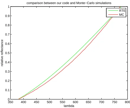
Our code has been compared to a reliable Monte-Carlo code that sends directly photons in the material (see [9] for more details). The following results have been obtained by setting in our code:
• [100,100,20] points for, respectively: epidermis, dermis, hypodermis,
• 160 angular samples for the whole sphere,
• 100 wavelengths, from 380 to 780 nm ,
• a tolerance of 10−7 for the convergence loop.
and by sending 10000 photons in the Monte-Carlo code.
Our simulation is based on the three main layers, whereas in the Monte-Carlo code, a multiplicative factor is used to take into account the full behaviour from the hypodermis. When a photon arrives at the dermis-hypodermis junction, it is either absorbed or reflected according to a pre-computed law. We show on the figure 2 the most delicate numerical experiment to reproduce. The optical index of the hypodermis has been carefully chosen to adjust the relative spectrum in a good agreement. We gain a time factor from 2 up to 3 in the good cases as opposed to the Monte-Carlo code.
350 400 450 500 550 600 650 700 750 800
−6 −4 −2 0 2 4 6 8
lambda
relative reflectance
comparison between our code and Monte−Carlo simulations
RTE MC
Figure 2. Relative reflectances for a given set of physiological parameters
350 400 450 500 550 600 650 700 750 800
0 0.1 0.2 0.3 0.4 0.5 0.6 0.7 0.8 0.9 1
lambda
relative reflectance
comparison between our code and Monte−Carlo simulations
RTE MC
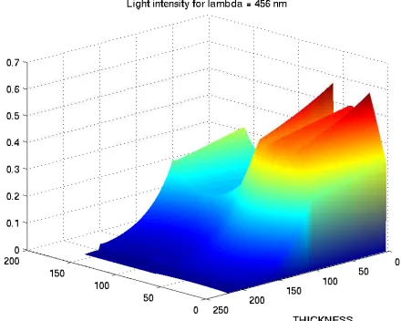
The figure 4 is a representation of the light intensity in the whole skin and for all the directions, for the wavelengthλ= 456 nm and for the following values of (µa, µs) in each layer: epidermis (1.69,88.43), dermis (0.985,260.11) and hypodermis (9.2720,1186.4).
Figure 4. Light intensity forλ= 456 nm
3.4.
Study of the derivatives
It would be interesting to retrieve the physiological parameters from the reflectance curve. To this end, we observe that the derivative of the intensity with respect to a parameterpi verifies the same transport equation with a given source term:
v· ∇x
∂f ∂pl
+σa
∂f ∂pl
=
Z
S2
k(v, w)∂f
∂pl
(x, w, λ) dw−∂σa ∂pl
f+
Z
S2 ∂k ∂pl
(v, w)f(x, w, λ) dw. (18)
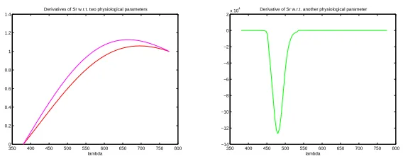
Hence the derivatives can be computed very easily from the same code and with the same scheme. So, once we have computed the light intensity, we use it in the source term of (18). From those derivatives, we can compute the derivatives of the reflectance curve with respect to each physiological parameter. On the figure 5, we present the derivatives of the reflectance curve with respect to three physiological parameters. This kind of result can help to understand in which range of wavelengths each component has a relative influence on the color of the skin. For example, looking at the right image, we can deduce that this physiological parameter has an influence on the color of the skin only for the wavelengths belonging to [450nm; 540nm].
We have to thank warmly Fran¸cois Golse, this article would not exist without his help. We also thank Caroline Magnain and Mady Elias for their help and their kindness. We are grateful to Yvon Maday, for his useful advises, and to Jorge Zubelli, for his help. Finally, we thank Emmanuel Grenier and Roberto Santoprete for their collaboration.
References
[1] G. Bal,Inverse transport theory and applications, Inverse Problems25, 053001, 2009
350 400 450 500 550 600 650 700 750 800 0
0.2 0.4 0.6 0.8 1 1.2 1.4
Derivatives of Sr w.r.t. two physiological parameters
lambda
350 400 450 500 550 600 650 700 750 800
−14 −12 −10 −8 −6 −4 −2 0 2x 10
4 Derivative of Sr w.r.t. another physiological parameter
lambda
Figure 5. Derivatives ofSr(λ) w.r.t. various physiological parameters
[3] M. Cessenat,Th´eor`emes de traceLppour des espaces de fonctions de la neutronique, C.R. Acad. Sci. Paris, S´erie I.299(1984), 831–834.
[4] M. Cessenat,Th´eor`emes de trace pour des espaces de fonctions de la neutronique, C.R. Acad. Sci. Paris, S´erie I.300(1985), 89–92.
[5] M. Choulli and P. Stefanov,An inverse boundary value problem for the stationary transport equation, Osaka J. Math36(1999), 87–104.
[6] R. Dautray and J.L. Lions, Analyse math´ematique et calcul num´erique pour les sciences et les techniques, Vol. 9, Masson, Paris, 1988.
[7] V. Isakov, Inverse problems for partial differential equations. 2nd edition. Applied Mathematical Sciences127, Springer, New York, 2006.
[8] K.P. Nielsen, L. Zhao, G.A. Ryzhikov, M.S. Biryulina, E.R. Sommersten, J.J. Stamnes, K. Stamnes and J. Moan,Retrieval of the physiological state of human skin from UV reflectance spectra, A feasibility study, Journal of Photochemistry and Photobiology B93(2008), 23–31.