J.-S. Dhersin, Editor
FIRST STEPS TOWARDS MORE NUMERICAL REPRODUCIBILITY
∗Fabienne J´
ez´
equel
1, Philippe Langlois
2and Nathalie Revol
3Abstract. Questions whether numerical simulation is reproducible or not have been reported in several sensitive applications. Numerical reproducibility failure mainly comes from the finite precision of computer arithmetic. Results of floating-point computation depends on the computer arithmetic precision and on the order of arithmetic operations. Massive parallel HPC which merges, for instance, many-core CPU and GPU, clearly modifies these two parameters even from run to run on a given computing platform. How to trust such computed results? This paper presents how three classic approaches in computer arithmetic may provide some first steps towards more numerical reproducibility.
1.
Numerical reproducibility: context and motivations
As computing power increases towards exascale, more complex and larger scale numerical simulations are performed in various domains. Questions whether such simulated results are reproducible or not have been reported more or less recently, e.g.in energy science [1], dynamic weather forecasting [2], atomic or molecular dynamic [3,4], fluid dynamic [5]. This paper focuses on numerical non-reproducibility due to the finite precision of computer arithmetic – see [6] for other issues about “reproducible research” in computational mathematics. The following example illustrates a typical failure of numerical reproducibility. In the energetic field, power system state simulation aims to compute at “real time” a reliable estimate of the bus voltages for a given power grid topology and a set of on-line measures. Numerically speaking, a large and sparse linear system is solved at every iteration of a Newton-Raphson process. The core computation is a sparse matrix-vector product automatically parallelised by the computing environment. The authors of [1] exhibit a significant variability (up to 25% relative difference) between two runs on a massively multithreaded system. The culprit? Here as in the previously cited references: non deterministic sums.
Floating-point summation is not associative. Parallelism introduces non deterministic events from run to run, even using a unique binary file and a given computing platform. The order of communications, the number of computing units (threads, processors) and the associated data placement may vary, and hence the parallel partial sums. Even sequential frames that comply with the IEEE-754 floating-point arithmetic standard [7] are still numerically very sensitive to many features: low-level arithmetic unit properties (variable precision registers, fused operators), compiler optimizations, language flaws or library versions reduce numerical repeatability and numerical portability [8].
∗ Authors thank Cl.-P. Jeannerod (INRIA) for his significant contribution, I. Said (LIP6) for his help in the numerical
experiments related to the acoustic wave equation and the GT Arith, GDR Informatique Math´ematique, for its support. 1Sorbonne Universit´es, UPMC Univ Paris 06, CNRS, UMR 7606, LIP6, F-75005, Paris, France and Universit´e Paris 2, France.
2Universit´e de Perpignan Via Domitia, DALI, LIRMM (UMR5506 CNRS-Universit´e Montpellier 2), France.[email protected]
3 INRIA, U. de Lyon, LIP (UMR5668 CNRS-ENS de Lyon-INRIA-UCBL), ENS de Lyon, France. [email protected]
c
EDP Sciences, SMAI 2014
Causes for such failures are numerous. So are the levels of an expected numerical reproducibility: from bit-wise identical results to debug or to verify contractual specifications, to a limited but guaranteed result accuracy to validate large scale simulations. Nevertheless numerical reproducibility failure is sometimes welcome as it may reveal a hidden bug. Of course numerical quality and running time or memory efficiency are contradictory goals that yield very different implementations in most cases.
Most of these failure causes are well known. Existing literature is not rare but spread over the concerned scientific communities: computer arithmetic, parallelism and HPC or over the numerous application domains [9]. Nevertheless the recent publications we mentioned at the beginning illustrate that the efficient control of their effects is still an open problem as exascale HPC allows application domain experts to trustfully simulate more and more realistic models. The aim of this paper is to present how three computer classic approaches in computer arithmetic may provide different response levels towards more numerical reproducibility.
Correct rounding, i.e. infinite precision rounded to a target format, ensures numerical reproducibility. An efficient and correctly rounded algorithm is very difficult to design and even moreto prove. Section 2 illustrates how to go further than the classic backward error analysis for small numerical kernels. Here an algorithm specifically designed to compute 2 by 2 determinants with IEEE-754 arithmetic is proved to always return an highly accurate result. Computing a set that encloses the infinite precision solution provides a safe reference
to validate non-reproducible computed results. Interval arithmetic is well known to return such set but, in practice, is implemented with floating-point arithmetic. Section 3 discusses how interval arithmetic faces the numerical reproducibility failures of its implementations and exhibits how to circumvent one important risk: the loss of the inclusion property when the rounding modes vary with respect to the computing platforms. Efficient validation with interval arithmetic needs more than oftenad hocalgorithms. Section 4 presents a more general probabilistic approach to estimate the local accuracy lost and so to localise some sources of numeri-cal non-reproducibility. Discrete stochastic arithmetic implemented in the CADNA library is applied to a 3D acoustic wave problem that suffers from different numerical reproducibility failures across CPU, GPU and APU.
Simulating an arbitrarily precise arithmetic is always possible: for instance double-double or quad-double libraries yield about twice or four times the IEEE-754 binary64 precision [10]. Most of the introductory references apply these libraries to improve numerical reproducibility without however avoiding all failure cases. Whereas they provide the first steps towards correct rounding, these libraries are not considered hereafter; the reader is invited to study [11] for details.
2.
Proving tight a priori bounds on round-off errors
Floating-point arithmetic as specified by the IEEE-754 standard is the most common way of dealing with real numbers on a computer. In numerical analysis, floating-point arithmetic is most often described in a simplified manner by the so-calledstandard model, which for each of the basic operations +,−,×,/,√ provides an upper bound on the rounding error possibly incurred by that operation. This model has been successfully used for more than 50 years to analyze a priori the numerical behavior of many algorithms, and especially linear algebra algorithms; see for example [12].
In particular, this model makes it possible to derive (in an efficient and elegant manner) some stability results and error bounds that are valid independently of the implementation of basic building blocks like sums of nfloating-point numbers or dot products of twon-dimensional vectors. In other words, sucha priori error bounds can be seen as a first step towards numerical reproducibility: depending on the context of computation (ordering, etc.), different results can (and, most of the time, will) be obtained, but we have at least the guarantee that they all share a same, common error bound.
exploiting “low-level” features in such cases makes it possible to derivea priori relative error bounds that are always tiny (that is, equal to a small integer multiple of the unit roundoff) and, therefore, to predict that for such kernels high relative accuracy is in fact always ensured.
2.1.
A reminder on IEEE floating-point arithmetic
The most recent specification of floating-point arithmetic is the 2008 revision of the IEEE-754 standard [7]. This standard, which has aimed since its initial 1985 version at better robustness, efficiency, and portability of numerical programs, specifies in particular the following issues.
• Floating-point data and their encoding into integers for various formats; • Results of operations on such data, as well as rounding-direction attributes; • Exceptional behaviors and how they should be handled;
• Conversions between formats.
Now we briefly comment on several of the above aspects; for thorough treatments, we refer to [8].
The data specified by IEEE-754-2008 consist of finite nonzero floating-point numbers and of special data. Finite nonzero floating-point numbers have the form
x= (−1)s·m·βe, (1)
where s ∈ {0,1} is the sign bit, m = Pp−1
i=0 miβ−i, mi ∈ {0,1, . . . , β −1}, is the significand, and e ∈
{emin, . . . , emax} is the exponent. Here, the integers β, p, emin, emax are the parameters defining the format
of such numbers: for example, the well-known binary64 format (double-precision) has radix β = 2, precision
p = 53, and extremal exponents emin = −1022 and emax = 1023. Furthermore, the number xis said to be
normal whenm06= 0, and subnormal whenm0 = 0 ande=emin. Special data consist of signed zeros +0 and
−0, infinities +∞and−∞, as well as not-a-numbers (NaN).
The result of operations like +, −, ×,/, √ must obey the so-calledcorrect rounding rule, which says that the operation is performed “as if to infinite precision” and then rounded to the target format. This requires to define how to round real numbers to floating-point data. IEEE-754 specifies five ways of doing so, via rounding-direction attributes: round to nearest (RN) with two different tie-breaking strategies, round towards zero (RZ), round towards +∞(RU), and round towards−∞(RD). The default way of breaking ties is “to even”, the other one being “to away”; see [7, §4.3.1]. Note also that even if round to nearest tends to be the default rounding mode in practice, the directed roundings RD and RU are essential for interval arithmetic; see Section 3.
Two specific features of the 2008 revision of IEEE-754 are worth being mentioned. First, thefused multiply-add (FMA) operation is now fully specified: given floating-point numbersa, b, c, this operation evaluates the expressionab+c with a single rounding instead of two. Second, correct rounding is recommended — yet, not required, for so-called elementary functions, which include functions like exp, cos,xn,p
x2+y2, and so on.
Finally, special data are a way of coping with exceptional behaviors. For example, if one of the operands of an operation is a NaN, or in cases like 0/0 or √−1, then the operation should be considered invalid and a NaN should be returned. Similarly, when the exact result of an operation lies outside the normal floating-point range, then either gradual underflow occurs and a subnormal number is returned, or overflow occurs and then ±∞or the smallest/largest representable number is returned.
2.2.
The standard model of floating-point arithmetic
The standard model is a simple and effective way of expressing the main feature of IEEE floating-point arithmetic: thanks to correct rounding and unless an exceptional behavior occurs, the result of any of the five basic arithmetic operations equals the exact result times a quantity close to 1. More precisely, given two normal floating-point numbersxandy, and given op∈ {+,−,×, /}, there existsinRsuch that
RN(xopy) = (xopy)(1 +), ||6u:=1 2β
Following [12, p. 40] we shall refer to (2) as the standard model of floating-point arithmetic. The same kind of equality holds for square root and the FMA. Here, the number uis the unit roundoff associated with the floating-point format under consideration. For the usual formats, it is a tiny value and thus 1 +≈1. Note also we have assumed in (2) that rounding is to nearest (RN). However, a similar model can be stated for directed roundings RZ, RD, RU, up to replacinguby 2u.
A key feature of (2) is to make it possible to consider the computed result as being the exact result of the same operation on slightly perturbed data. For example, RN(x+y) equals the exact sumxe+ye, wherexe=x(1 +) and ye=y(1 +) are real numbers whose relative distance to x and y, respectively, is bounded by u. Using this feature repeatedly is at the heart of Wilkinson’s backward error analysis[13, 14]. As an example, consider the evaluation (with + and×and in any order) of the dot productr=Pn
i=1xiyi. Assuming that underflows
and overflows do not occur, we can apply (2) to each of the 2n−1 operations involved and deduce that the computed solution satisfiesrb=Pn
i=1xiyi(1 +i), where fori= 1, . . . , n,|i|6(1 +u)n−1 =nu+O(u2). This
equality says bris the exact dot product of slight real perturbations of the initial floating-point vectors. For r
nonzero, it leads further to the forward relative error bound
|rb−r|
|r| 6 (1 +u)
n
−1 Pn
i=1|xiyi|
|r| . (3)
WhenPn
i=1|xiyi| |r|, such a bound can be larger than 1. However, this agrees withbrhaving no correct digit
at all, because of possible catastrophic cancellations occurring when adding the nproducts.
Let us now consider a second example, namely, Kahan’s algorithm for 2 by 2 determinants [12, p. 60], where just using the standard model (2) is not enough to obtain a satisfactory error bound. Given floating-point numbersa, b, c, d and assuming that an FMA is available, Kahan’s algorithm evaluatesr=ad−bcas follows:
b
w:= RN(bc); fb:= RN(ad−wb); e:= RN(wb−bc); br:= RN(fb+e).
The operation producing ebeing exact [15], it can be checked by applying the standard model (2) to each of the 3 remaining operations that the computed result brsatisfies
|br−r|
|r| 6(2u+u 2)
1 +u|bc| 2|r|
. (4)
Hence this bound implies high relative accuracy as long as u|bc| 62|r|, and when the ratio u2||bcr|| is huge, one could believe that the error itself can be very large too. In fact, as shown in [16], the latter situation turns out to be impossible. However to prove Kahan’s algorithm is always highly accurate, it is not enough to use just the standard model (2) and the exactness ofe: further properties of floating-point arithmetic must be exploited.
2.3.
Exploiting “low-level” features of IEEE floating-point arithmetic
In addition to (2), the IEEE-754 specification confers many nice properties to floating-point arithmetic, thanks to the special shape (1) of floating-point numbers and to the fact that rounding r ∈ R to nearest satisfies, by definition, |RN(r)−r|6|x−r| for all floating-point numbersx. Such properties include the fact that ifxopy is a floating-point number then= 0, the fact that RN commutes with the absolute value and is nondecreasing, or the fact that floating-point multiplication by an integer power of the radixβ is exact. Some other properties heavily depend on the notion ofunit in the last place(ulp) [8,§2.6.1]: in particular, givenr∈R
and in the absence of underflow and overflow, the following tighter bound implies the standard model (2):
|RN(r)−r|6ulp(r)/26u|r|.
In Kahan’s algorithm, the error terms1:=fb−(ad−wb) and2:=rb−(fb+e) can be analyzed tightly thanks
to those “lower-level” properties: as proved in [16], both|1|and|2|are bounded by β2ulp(r) and, on the other
in practice β is 2 or 10, the bound 2βu thus already ensures that Kahan’s algorithm always has high relative accuracy, in contrast to (4). However, this bound is still sub-optimal and it is shown further in [16] that
|rb−r| |r| 62u
for all radix β >2, and that this bound is tight. Thus, a careful use of ulp properties and of various other “lower-level” features of IEEE-754 arithmetic made it possible to prove that a numerical kernel like Kahan’s 2 by 2 determinant always behaves ideally in the absence of underflow and overflow. This was far from obvious when resorting exclusively to the standard model.
3.
Validating numerical results with interval arithmetic
Interval arithmetic is a tool of choice when it comes to guaranteeing the result of a numerical computation. Indeed, interval computations return intervals which are enclosures of the exact results, if the inputs are intervals enclosing the data. This holds true even when floating-point arithmetic is used and round-off errors enter the scene, and even when numerical computations are not performed reproducibly. When the numerical computation is not reproducible, that is, when several runs produce different results, these results can be compared against the interval result.
3.1.
Introduction to interval arithmetic
Interval computations handle intervals, not numbers. An interval can be the enclosure of some physical datad, measured with, say, absolute error at mostδ: in this case the corresponding interval is [d−δ, d+δ]. An interval can also be used to process a value that is not finitely representable, such as π: the interval [3.1415,3.1416] containsπ, it is finitely representable in decimal arithmetic and it can easily be manipulated. Finally, intervals can be used to handle whole ranges of values, to compute with sets.
Computations can be performed on intervals. An interval that appears as an intermediate or final quantity in a computation is an enclosure of the range of possible values for the corresponding numerical quantity. Let us put it more explicitly. In interval arithmetic, the fundamental theorem is the inclusion property: the exact result, be it a number or a set, is contained in the computed interval. It is guaranteed that no result is lost,i.e.
lies outside the interval.
If the input data satisfy the inclusion property, it is possible to perform subsequent operations and compu-tations in a way that preserves the inclusion property. Let us give two examples, the addition and the division. In what follows, let us denote intervals using boldface letters and let us represent them by their endpoints. An interval a is a subset of R and a = [a,¯a] = {a : a ≤ a ≤ ¯a} with a ∈ R∪ {−∞}, ¯a ∈ R∪ {+∞} and
a ≤¯a. Let a = [a,¯a] and b= [b,¯b] be two intervals. The addition c =a+bis obtained using the formula
c= [c,¯c] = [a+b,a¯+ ¯b],i.e.c=a+band ¯c= ¯a+ ¯b. Ifa630, then the inverse 1/ais given by 1/a= [1/a,¯ 1/a]. These examples illustrate that it is possible to compute with intervals. The general definition ofab, where is any mathematical operation, is
ab= Hull{ab, a∈a, b∈b},
where Hull is the convex hull of the set: this ensures that the result is an interval, without gaps. As it can be seen on the formulas for addition and inversion, using the monotonicity leads to practical formulas for the implementation of operations. For more details about interval arithmetic, see [17, 18] for instance.
Frequently, interval arithmetic is implemented on computers using the floating-point arithmetic available on these machines. To preserve the inclusion property, directed roundings (introduced in Section 2.1) of the endpoints are used. For instance, the formulas for the addition and the division become
As already mentioned, the main advantage of interval arithmetic is to offer a guarantee: the computed intervals are guaranteed to contain the exact results. It is also said that interval arithmetic returns verified enclosures of the results. It has been hoped, in the early years of interval arithmetic, that it would in particular provide a guarantee on the numerical accuracy of a result computed using floating-point arithmetic,i.e.that it would give the error due to round-off. Unfortunately, this is not the case: replacing, in a numerical code, the floating-point datatype by the interval datatype may produce very large intervals. Indeed, interval computations suffer from overestimation and such a naive use of interval arithmetic is very likely to yield to a blow-up of the interval widths. Let us illustrate the problem with the simplest example possible. Computinga−a does not result in {0}, as with real or floating-point arithmetic, but in an interval whose width is twice the width ofa. Let us use the definition of an operation to understand the problem:
a−a= Hull{a1−a2, a1∈a, a2∈a}= [a−¯a,¯a−a].
What this example illustrates is the so-called variable dependency problem: it is not known whethera1 and
a2 correspond to the same variable or not, and thus to the same value in a or not. This example is not
contrived: Karatsuba’s formula for the multiplication of polynomials is (a1x+a0)·(b1x+b0) = a1b1x2+
((a1+a0)(b1+b0)−a1b1−a0b0)x+a0b0,and, therefore, exploits the fact thata1b1−a1b1=a0b0−a0b0= 0,
which does not hold true in interval arithmetic. Strassen’s algorithm for fast matrix multiplication is similar. Two main families of techniques are commonly used to reduce this interval’s swelling. A brute force approach, which is often used as a last resort, consists in bisecting the input intervals in smaller subintervals, and in performing the computations on these subintervals. The final result is the union of the sub-results. It is known [17,§2.1] that the width of the result is proportional to the width of the input: this justifies the bisection technique. Another family of techniques consists in employing more elaborate variants of interval arithmetic, designed to reduce the dependency problem. Let us cite briefly slope and other so-called centered forms [17,§2.3], affine arithmetic [19, 20], Taylor models [21] among the most used ones. Algorithms are designed specifically for interval computations and most of them usually combine both kinds of techniques.
3.2.
Interval arithmetic and reproducibility issues: when the inclusion property is at risk
As interval arithmetic is usually implemented using floating-point arithmetic, it is subject to the same issues, regarding numerical reproducibility, as floating-point arithmetic. The main issues, as introduced in Section 1, are variable computing precision and variable order of the operations. It is also subject to specific issues, in particular the order, not only of the arithmetic operations but also of the bisections of intervals. Interval arithmetic is sensitive to numerical reproducibility issues: the computed result may differ from one run to the next. Still, it is always guaranteed to be an enclosure of the result. However, in some cases, this guarantee can be lost. Indeed, other issues regarding numerical reproducibility of interval computations threaten the inclusion property.
3.3.
How to preserve the inclusion property
The inclusion property can be lost due to the unavailability of directed rounding modes. The inclusion property can therefore be recovered by becoming independent of the rounding mode. Indeed, interval arithmetic can be implemented with the default rounding to nearest. This can be done by enlarging the computed interval, as in the early version of the FI LIB library [22] for instance: for each operation, the last bit of the left endpoint was decreased by 1, and similarly the right endpoint was slightly shifted right. Some experiments indicate that the loss of accuracy is limited: it roughly corresponds to computing with a precision of 52 bits instead of 53 in binary64. Another approach, promoted in [23] and here, consists in determining bounds on the round-off errors, such as bounds given in (3) for the dot product, and by shifting the endpoints by this amount. However, the bound given in (3) uses real arithmetic, whereas we need an upper bound that can be computed with floating-point arithmetic. Let us take the example of the dot product: the idea is to enlarge every operand |xi| and |yi| by a multiplicative factor — and we suggest to use the factor 1 + 4u, which is
a floating-point number —, and to perform a floating-point multiplication. Subsequently, the floating-point product RN(RN((1 + 4u)· |xi|)·RN((1 + 4u)· |yi|)) is an upper bound of |xiyi|. Eventually the sum, in any
order, of these products is an upper bound ofPn
i=1|xiyi|. Similarly, a floating-point multiplication by a term
slightly larger than (1 +u)n−1
ensures that an upper bound on the right hand-side of (3) has been obtained, by resorting solely to floating-point arithmetic. It can even be obtained by using any optimized numerical routine for the dot product, where the input vectors are (RN((1 + 4u)· |xi|))1≤i≤nand (RN((1 + 4u)· |yi|))1≤i≤n.
A similar method is given in [23] for the product of matrices. What this dot product exemplifies is the fact that the inclusion property can be preserved even when the only available mode is rounding to nearest (RN), and that interval computations can even benefit from optimized numerical routines. The only condition is that these bounds must hold independently of issues related to numerical reproducibility: in particular, they have to hold independently of the order of the operations.
4.
Estimating round-off errors with discrete stochastic arithmetic
Differences between the results of a code can be observed from one architecture to another or even inside the same architecture. In this section, we show how to estimate round-off errors which lead to such differences. The aim here is not to force a code to be reproducible, but to estimate the number of digits in the results which may be different from one execution to another because of round-off errors. This approach is illustrated by a wave propagation code which can be affected by reproducibility problems.
4.1.
Reproductibility failures in a wave propagation code
We consider the three-dimensional acoustic wave equation 1
c2
∂2u
∂t2 − P
b∈{x,y,z}
∂2
∂b2u = 0, where u is the
particle velocity,cis the wave velocity, andtis the time. This equation, used for instance in oil exploration [24], is solved with a finite difference scheme of order 2 in time andpin space (in our casep= 8).
Two mathematically equivalent implementations of the finite difference scheme are proposed:
unijk+1= 2unijk−unijk−1+c
2∆t2
∆h2
p/2 X
l=−p/2
al uni+ljk+u n
ij+lk+u n ijk+l
+c2∆t2fijkn , (5)
unijk+1= 2unijk−unijk−1+c
2∆t2
∆h2
p/2 X
l=−p/2
aluni+ljk+ p/2 X
l=−p/2
alunij+lk+ p/2 X
l=−p/2
alunijk+l
+c 2∆t2fn
whereun
ijk (respectivelyf n
ik) is the wave (respectively source) field in (i, j, k) coordinates andnth time step and
al,l=−p/2, . . . , p/2, are the finite difference coefficients.
The code is executed for 64×64×64 space steps and 1000 time iterations in IEEE-754 binary32 arithmetic with rounding to the nearest and the following CPU, GPU and APU (Accelerated Processing Unit): i) Intel i7-3687U CPU with gcc 4.6.3 compiler; ii) NVIDIA K20c GPU (Graphics Processing Unit) with OpenCL (Open Computing Language); iii) AMD Radeon HD 7970 GPU with OpenCL; iv) AMD Trinity APU with OpenCL.
Different kinds of reproducibility problems are observed. The results numerically vary
(1) from one execution to another inside a GPU or an APU; these repeatability problems are due to differences in the execution order of the threads;
(2) from one implementation of the finite difference scheme to another; the maximal relative difference between results is of the order of 10−1 to 1 depending on the architecture, and the mean value of the relative difference between results is of the order of 10−5whatever the architecture;
(3) from one architecture to another; again, the maximal relative difference between results is of the order of 10−1 to 1 and its mean value is 10−5.
Therefore, if two sets of results computed in binary32 are compared, the results at the same space coordinates can have from 0 to 7 significant digits in common, and the average number of common significant digits is about 4. We recall that the binary32 arithmetic precision is about 8 digits.
4.2.
Principles of discrete stochastic arithmetic (DSA)
Based on a probabilistic approach, the CESTAC method [25] allows the estimation of round-off error propa-gation which occurs with floating-point arithmetic. When no overflow occurs, the exact result of any non exact floating-point arithmetic operation is bounded by two consecutive floating-point valuesR− andR+. The basic
idea of the method is to perform each arithmetic operation N times, randomly rounding each time, with a probability of 0.5, toR− orR+. The computer’s deterministic arithmetic, therefore, is replaced by a stochastic
arithmetic where each arithmetic operation is performedNtimes before the next one is executed, thereby prop-agating the round-off error differently each time. The CESTAC method furnishes us withNsamplesR1, . . . , RN
of the computed resultR. The value of the computed result,R, is the mean value of{Ri}16i6N and the number
of exact significant digits inR,CR, is estimated as
CR= log10 √
NR
στβ
!
, where R = 1 N
N X
i=1
Ri andσ2=
1 N−1
N X
i=1
Ri−R 2
. (7)
τβ is the value of Student’s distribution forN−1 degrees of freedom and a probability level 1−β. In practice
N = 3,β = 0.05 and thenτβ= 4.303.
The validity ofCRis compromised if the two operands in a multiplication or the divisor in a division are not significant [26]. It is essential, therefore, that any computed result with no significance is detected and reported, since its subsequent use may invalidate the method. The need for this dynamic control of multiplications and divisions has led to the concept of the computational zero. A computed result is a computational zero, denoted by @.0, if ∀i, Ri = 0 or CR ≤ 0. This means that a computational zero is either a mathematical zero or a
number without any significance, i.e. numerical noise.
To establish consistency between the arithmetic operators and the relational operators, discrete stochastic relations are defined as follows. LetX andY be two computed results, we have from [27]
X =Y if X−Y = @.0; X>Y if X>Y and X−Y6= @.0; X≥Y if X≥Y or X−Y = @.0. (8)
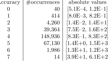
Table 1. Accuracy, number of occurrences, and range of the absolute values of the results.
Accuracy #occurrences absolute values 0 40 [5.1E–4, 1.2E–1] 1 414 [8.0E–3, 8.2E–1] 2 4,260 [1.4E–2, 1.4E+1] 3 39,364 [7.5E–2, 1.6E+2] 4 148,936 [8.3E–1, 8.3E+2] 5 67,130 [1.4E+0, 1.5E+3] 6 1,986 [1.3E+1, 1.2E+3] 7 14 [3.9E+1, 6.1E+2]
The CADNA software [28] is a library which implements DSA in any code written in C++ or in Fortran and allows to use new numerical types: the stochastic types. In practice, classic floating-point variables are replaced by the corresponding stochastic variables, which are composed of three perturbed floating-point values. The library contains the definition of all arithmetic operations and order relations for the stochastic types. The control of the accuracy is performed only on variables of stochastic type. Only significant digits of a stochastic variable are printed or “@.0” for a computational zero. Because all operators are overloaded, the use of CADNA in a program requires only a few modifications: essentially changes in the declarations of variables and in input/output statements. CADNA can detect numerical instabilities which occur during the execution of the code. When a numerical instability is detected, dedicated CADNA counters are incremented. At the end of the run, the value of these counters together with appropriate warning messages are printed on standard output.
4.3.
Estimation of numerical reproducibility by means of DSA
The CPU version of the acoustic wave propagation code is examined with the CADNA library. With im-plementations (5) and (6) of the finite difference scheme, the number of exact significant digits in the results varies from 0 to 7, and its mean value is 3.6. This remark is consistent with the observations described in Section 4.1. Numerical instabilities are detected during the executions: 272,394 losses of accuracy due to can-cellations with scheme (5) and 285,186 with scheme (6). These instabilities are detected if the subtraction of two close floating-point numbers leads to a loss of accuracy of at least four digits.
Table 1 presents the number of exact significant digits estimated by CADNA for scheme (5), the occurrence number of each accuracy, and the absolute value range of the analysed results. Similar results are observed with the other scheme. The highest results (in absolute value) are affected by low round-off errors and the highest round-off errors impact negligible results.
References
[1] O. Villa, D. G. Chavarr´ıa-Miranda, V. Gurumoorthi, A. M´arquez, and S. Krishnamoorthy. Effects of floating-point non-associativity on numerical computations on massively multithreaded systems. InCUG 2009 Proceedings, pages 1–11, 2009. [2] Y. He and C.H.Q. Ding. Using accurate arithmetics to improve numerical reproducibility and stability in parallel applications.
The Journal of Supercomputing, 18:259–277, 2001.
[3] M. A. Cleveland, T. A. Brunner, N. A. Gentile, and J. A. Keasler. Obtaining identical results with double precision global accuracy on different numbers of processors in parallel particle Monte Carlo simulations.Journal of Computational Physics, 251(0):223 – 236, 2013.
[4] M. Taufer, O. Padron, Ph. Saponaro, and S. Patel. Improving numerical reproducibility and stability in large-scale numerical simulations on GPUs. InIPDPS, pages 1–9. IEEE, 2010.
[5] R. W. Robey, J. M. Robey, and R. Aulwes. In search of numerical consistency in parallel programming.Parallel Computing, 37(4-5):217–229, 2011.
[6] V. Stodden, D. H. Bailey, J. Borwein, R. J. LeVeque, W. Rider, and W. Stein. Setting the default to reproducible: Repro-ducibility in computational and experimental mathematics. Technical report, ICERM, February 2013.
[7] IEEE Computer Society.IEEE Standard for Floating-Point Arithmetic. IEEE Standard 754-2008, August 2008.
[8] J.-M. Muller, N. Brisebarre, F. de Dinechin, C.-P. Jeannerod, V. Lef`evre, G. Melquiond, N. Revol, D. Stehl´e, and S. Torres. Handbook of Floating-Point Arithmetic. Birkh¨auser Boston, 2010.
[9] N. Revol and Ph. Th´eveny. Numerical reproducibility and parallel computations: Issues for interval algorithms.IEEE Trans-actions on Computers, 63(8):1915–1924, August 2014.
[10] URL =http://crd.lbl.gov/~dhbailey/mpdist, .
[11] D. H. Bailey, R. Barrio, and J. M. Borwein. High-precision computation: Mathematical physics and dynamics.Applied Math-ematics and Computation, 218(20):10106–10121, 2012.
[12] N. Higham.Accuracy and Stability of Numerical Algorithms. SIAM, (2nd edition), 2002.
[13] J. H. Wilkinson.Rounding Errors in Algebraic Processes. Notes on Applied Science No. 32, Her Majesty’s Stationery Office, London, 1963. Also published by Prentice-Hall, Englewood Cliffs, NJ, USA. Reprinted by Dover, New York, 1994.
[14] J. H. Wilkinson.The Algebraic Eigenvalue Problem. Oxford University Press, 1965.
[15] W. Kahan. Lecture notes on the status of IEEE Standard 754 for binary floating-point arithmetic. Manuscript, May 1996. [16] C.-P. Jeannerod, N. Louvet, and J.-M. Muller. Further analysis of Kahan’s algorithm for the accurate computation of 2×2
determinants.Mathematics of Computation, 82:2245–2264, 2013.
[17] A. Neumaier.Interval Methods for Systems of Equations. Cambridge University Press, 1990.
[18] W. Tucker.Validated Numerics: A Short Introduction to Rigorous Computations. Princeton University Press, 2011. [19] J. Stolfi and L. H. de Figueiredo. Self-validated numerical methods and applications. InMonograph for 21st Brazilian
Mathe-matics Colloquium, IMPA, Rio de Janeiro, 1997.
[20] L. H. de Figueiredo and J. Stolfi. Affine arithmetic: concepts and applications.Numerical Algorithms, 37:147–158, 2004. [21] K. Makino and Berz. M. Taylor models and other validated functional inclusion methods.International Journal of Pure and
Applied Mathematics, 4(4):379–456, 2003.
[22] W. Hofschuster and W. Kr¨amer. FI LIB - A fast interval library (Version 1.2) in ANSI-C, 2005. http://www2.math. uni-wuppertal.de/~xsc/software/filib.html.
[23] S. M. Rump. Fast interval matrix multiplication.Numerical Algorithms, 61(1):1–34, 2012.
[24] H. Calandra, R. Dolbeau, P. Fortin, J.-L. Lamotte, and I. Said. Forward seismic modeling on AMD Accelerated Processing Unit. InRice Oil & Gas HPC Workshop, Houston, TX, USA, March 2013.
[25] J. Vignes. A stochastic arithmetic for reliable scientific computation.Math. Comput. Simulation, 35:233–261, 1993.
[26] J.-M. Chesneaux.L’arithm´etique stochastique et le logiciel CADNA. Habilitation `a diriger des recherches, Universit´e Pierre et Marie Curie, Paris, France, November 1995.
[27] J.-M. Chesneaux and J. Vignes. Les fondements de l’arithm´etique stochastique.C. R. Acad. Sci. Paris S´er. I Math., 315:1435– 1440, 1992.
[28] F. J´ez´equel and J.-M. Chesneaux. CADNA: a library for estimating round-off error propagation.Computer Physics Commu-nications, 178(12):933–955, 2008.
[29] S. Montan and C. Denis. Numerical verification of industrial numerical codes. InESAIM, volume 35, pages 107–113, 2012. [30] F. J´ez´equel and J.-L. Lamotte. Numerical validation of Slater integrals computation on GPU. In14th International Symposium