Jean-Fr´ed´eric Gerbeau & St´ephane Labb´e, Editors
A GLUEY PARTICLE MODEL
B. Maury
1Abstract. We present here a new framework to handle the short-range interaction between rigid bodies in a viscous, incompressible fluid. This framework is built as the vanishing viscosity limit of a lubrication model. We restrict ourselves here to the case of a single particle and a rigid wall. Our approach is based on a standard first-order approximation for the lubrication force between two rigid bodies, where a small parameterεplays the role of the underlying fluid viscosity. We establish
convergence whenε goes to 0 of a subsequence of trajectories towards a solution to a problem of the
hybrid type: it relies on two distincts states, unglued and glued, the latter being described by a new variableγ which expresses in a way the asymptotic smallness of the distance, and which plays the role
of an adhesion potential. The limit problem has a surprising property: although it is well-posed in many situations, uniqueness does not generally hold as soon as left-hand clusters of contact times are allowed. Some prospective extensions of this model (other types of singularities, roughness of surfaces, macroscopic version) are proposed.
R´esum´e. Nous pr´esentons ici un nouveau cadre pour g´erer l’interaction `a courte port´ee entre corps rigides baignant dans un fluide visqueux. Notre mod`ele est construit comme la limite `a viscosit´e ´evanescente d’un mod`ele de lubrification. Nous nous restreignons ici au cas d’une sph`ere unique au voisinage d’une paroi plane. Le point de d´epart de notre approche est ainsi un mod`ele qui estime au premier ordre les forces de lubrification entre une sph`ere et un plan en quasi-contact, mod`ele dans lequel un petit param`etreεjoue le rˆole de la viscosit´e du fluide environnant. Nous montrons la convergence,
quandεtend vers 0, d’une sous-suite de solutions vers une solution d’un probl`eme de type hybride. Ce
mod`ele limite se base sur la d´efinition de deux ´etats, libre et coll´e, ce dernier ´etat ´etant d´ecrit par une nouvelle variableγ qui repr´esente d’une certaine mani`ere la petitesse asymptotique de la distance, et
qui joue le rˆole d’un potentiel d’adh´esion. Le probl`eme limite jouit d’une propri´et´e surprenante : bien qu’il soit bien pos´e dans un grand nombre de situations, on n’a pas unicit´e en g´en´eral d`es que l’on sort du cadre d’instants de contact isol´es. Nous pr´esentons pour finir des extensions possibles de ce travail (autres types de singularit´e, prise en compte de la rugosit´e, version macroscopique du mod`ele).
1.
Introduction, finite viscosity lubrication model
We are interested in the behaviour, as εgoes to 0, of the solutionqεto
¨
qε=−εqε˙ qε +f(t),
qε(0) =q0>0, qε˙ (0) =u0,
(1)
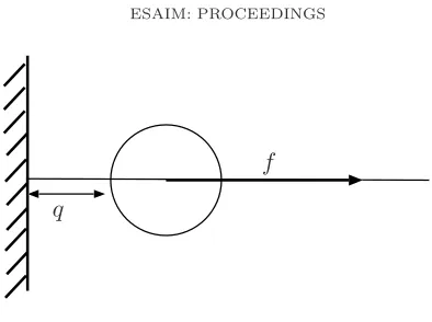
wheref is a given forcing term. It models the motion of a solid sphere of unit mass in a viscous fluid, subject to move horizontally on thex-half line, in the neighbourhood of the planex= 0 corresponding to a solid wall (see
1 Laboratoire de Math´ematiques, Universit´e Paris Sud, 91405 Orsay cedex. e-mail:[email protected]
c
EDP Sciences, SMAI 2007
q
f
Figure 1. Geometry.
Fig.1). The interaction force which results from the three dimensional lubrication flow in the gap between a ball and a plane can indeed be proved to behave like the product of the reciprocal of the wall-particle distance, the relative velocity, and the viscosity of the surrounding fluid (see [5, 7]).
The main purpose of this paper is to establish convergence of the solution to this ODE, when ε goes to 0, towards a solution to an evolution problem of the hybrid type. Indeed, the description of the asymptotic behaviour calls for the use of an extra variable γwhich is activated when contact occurs. This new variableγ
makes it possible to include memory effects in the limit model: it keeps track of the sollicitations undergone by the sphere as long as it is stuck to the wall. As we shall see, γ measures in a way the asymptotic smallness of the wall-particle distance, and yet it follows the same equation as the one the velocity would obey if there were no obstacle.
As a first step, we prove well-posedness of Problem (1), which is a straightforward consequence of the fact that the sphere never touches the wall:
Proposition 1.1. Let ε > 0 and f ∈ L1
loc(R
+) be given. Then Problem (1) admits a unique global solution
qε∈W1,∞
loc (R
+).
Proof. The local Lipschitz character of (q, u)7→u/qin ]0,+∞[×Rensures existence and uniqueness of a maximal
solution to (1), defined over the time interval [0, τ[. Lipschitz regularity of this solution is a consequence of the standard energy estimate combined with Gronwall Lemma:
1 2|qε|˙
2≤1
2|qε|˙
2+εZ t 0
|qε|˙ 2
qε ≤
1 2|u
0|2+Z t 0
|f||qε|˙ =⇒ |qε| ≤ |u˙ 0|+ Z t
0
|f|. (2)
From this estimate, we also get that the velocity ˙qεcannot blow up within a finite time, so that, ifτ <∞, then necessarilyqε goes to 0 astgoes toτ−
. Integration of (1) gives
˙
qε(t) =u0−εln qε(t)
q0
+
Z t
0
f(s)ds,
so thatqε→0 implies ˙qε(t)7→+∞, hence a contradiction.
Remark 1.2. Note that this no-contact property does no longer hold as soon as the lubrication force is weakened. For instance, if −εqε/qε˙ is replaced by −εqε/q˙ 1−η
ε , with η > 0, then contact may occur within a
finite time, and the previous proposition, as well as the rest of the paper, is invalidated. On the other hand, more singular forces like−εqε/q˙ 1+η
2.
Asymptotic behaviour
Let us denote by I the time interval ]0, T[. Our aim is to establish convergence (up to a subsequence) of
qε towards a function q which is a solution to a problem of the hybrid type onI. We shall first describe the limit problem in three different forms, which are formally equivalent. The first one, on which the convergence theorem2.1shall be based upon, is the following:
Find q∈W1,∞(I), γ∈L∞(I), such that
˙
q+γ= ˜u=u0+ Z t
0
f(s)ds a.e. inI ,
γ≤0, q≥0, qγ= 0 a.e. inI ,
q(0) =q0>0, q˙(0) =u0.
(3)
As we shall see in Section4, this problem may admit multiple solutions in general, and it is not a matter of regularity conditions onf: as suggested by counter-examples for granular flow models, only analyticity can be expected to provide uniqueness,f ∈C∞
being not sufficient (see [1, 10, 11]).
Yet, it is somehow well-posed in the sense that, in many situations, a solution can be built in a unique way. Let us describe a heuristic procedure to build a solution. At first, the system behaves as if there were no wall,
q is positive and thereforeγ is 0. Note that q cannot drop abruptly to 0, for continuity is required. Let us assume that the unconstrained pathline would become negative for the first time right after some timeτ1>0.
It is not possible forqto become negative, and thereforeq is stuck to the value 0, whereasγis activated right afterτ1, and is defined byγ= ˜u. As far asγremains negative,qremains glued on the wall, andγcan not jump
abruptly from a negative value to 0 because, if it did,qwould restart with a negative velocity ˜u, henceqwould actually enter the wall. Therefore, γgoes smoothly to 0 from below, and when it hits 0 at timeτ2,qtakes off
from the wall. Fig. 2presents an example of such a behaviour. Note that this approach cannot be carried out in the neighbourhood of cluster points of hitting times.
Problem (3) can be expressed in the spirit of granular flow models (see [1, 10]). The formulation we propose now is close to (3), with the difference that the interaction force between the wall and the particle is explicited. based on this second formulation. It reads
Findq∈W1,∞
(I) with ˙q∈BV(I), γ∈BV(I), µ∈ M(I), such that ¨
q=f+µin M(I),
supp(µ)∈ {t, q(t) = 0},
˙
q+=PC qq˙
−,
˙
γ=−µ ,
γ≤0, q≥0, qγ= 0 a.e. inI , q(0) =q0>0, q˙(0) =u0,
(4)
whereM(I) denotes the set of bounded measures onI, BV(I) the set of functions with bounded variation over
I, ˙q+(resp. ˙q−
), is the right limit (resp. left limit) of ˙q, andCq is the convex cone of feasible velocities, defined by
Cq=
R if q >0, R
+ if q= 0 andγ−
= 0, {0} if q= 0 andγ−
<0.
Before stating the convergence result, let us mention a third, event-driven formulation, which formalizes the heuristic procedure to build up a solution given above. It is based on the introduction of two distinct states for the system, indexed by 0 (unglued, the particle does not touch the wall,q >0) and 1 (glued, the particle is in contact with the wall,q= 0 andγ <0). Borrowing the terminology of [6], we introduce the set of statesQ, the collection of domains (D), of forcing terms (F), of jump sets (G), and the transition mapsR01 andR10:
Q={0,1}, D= (D0, D1) = ((R
+×
R),R
−
), X0=
q u
, X1=γ ,
F = (F0, F1) =
u f
,[f]
,
G01=
0
R
−
, G10={0}, R01
0
u
=u , R10(0) =
0 0 . (5)
This hybrid framework describes the following behaviour: Starting fromq0>0 att= 0, the system is in state
0, so that the domain isD0, and the state variableX0= [q, u]tverifies
˙
X0=F0(X0), namely
˙ q ˙ u = u f .
As soon as G01 is hit (i.e. as soon as q = 0), at a certain time τ1 >0, the system switches to states 1, and
the new variableX1, which is γ in the previous notations, is set toR01(X0(τ1−)), which is the value ofuright
before the contact. The system continues with the new dynamic
˙
X1=F1(X1), namely ˙γ=f,
untilG10={0}is hit, making the system switch back to state 0 (the particle is free to take off the wall).
We may now state the convergence result, which refers to the formulation (3) of the limit problem.
Theorem 2.1. Letq0>0,u0∈
R, a time intervalI=]0, T[andf ∈L
1(I)be given. We denote byqε∈W1,∞
(I) the unique solution to (1) in I, and we set γε = εlnqε . When ε goes to 0, there exists a subsequence, still denoted by(qε),q∈W1,∞(I),γ∈L∞
(I), such that
qε −→ q uniformly , γε −⋆⇀ γ inL∞
weak−⋆,
and the couple (q, γ)is a solution to Problem (3).
Proof. Boundedness of (qε) inW1,∞
(I) is a direct consequence of (2) (see the proof of Prop.1.1). Consequently, one can extract a subsequence (still denoted byqε) such thatqεconverges uniformly to someq∈W1,∞
, and ˙qε
converges tou= ˙qin the weak-⋆sense.
Letγεbe defined asεlnqε. Straightforward computations give
˙
qε+γε=u0+γε0+ Z t
0
f,
where γ0
ε =γε(0) = εlnq0 goes to 0 with ε. As a consequence, γε converges weak-⋆ in L ∞
towards γ ∈L∞
such that
˙
q+γ=u0+ Z t
0
The next step consists in proving thatqis such that ˙q= ˜uinI0={t, q(t)>0}. To that purpose we introduce,
for anyη >0, the set Iη(q) ={t∈]0, T[, q(t)> η}. Asqε converges uniformly toq, one has Iη(q)⊂Iη/2(qε)
forεsufficiently small. As a consequence,γε=εlnqεgoes uniformly to 0 onIη(q), thus ˙qεconverges uniformly towards the unconstrained velocity ˜uin Iη(q), for allη >0. The limitqis thereforeC1 onI
0, with ˙q= ˜u, and
γ is identically 0 onI0.
On Ic
0(q) ={t, q(t) = 0}, q is constant, so that ˙q= 0 almost everywhere, thus γ = ˜ua.e. Beside, asγε is
negative as soon asqεis less than 1, one hasγ≤0 onIc
0.
3.
Numerical illustration
This section presents some computations to illustrate the convergence ofqε (resp. γε) towardsq (resp. γ). As it is not the point of this paper to go deep into numerical considerations, we shall simply describe the algorithms we used to run the numerical tests. Firstly, the numerical computation of (1), forε >0, is based on a semi-implicit Euler scheme applied to the integrated equation forγε=εlnqε (we drop the subscriptεfor readability reasons):
˙
q=−εln q
q0+ ˜u=⇒γ˙ =εe
−γ/ε(˜u−γ),
and the latter equation is discretized by
γn+1−γn h =εe
−γn/ε
(˜u(tn+1)−γn+1)
which can also be written
γn+1=θγn+ (1−θ) ˜u(tn+1) with θ= 1 1 +hεe−γn/ε.
Note how the latter form exhibits the hybrid behaviour: whenθ is close to 1 (γ close to 0, unglued case),γn
does not vary much, whereas whenθ is close to 0 (γ negative, glued case), the approximation ofγfollows ˜u. As for the hybrid formulation, we used the following scheme: with tn = nh. Assuming qn, un, and γn
are known at time step tn, the next values are computed according to the following alternative (depending on
whether the contact is active or not):
ifqn >0
un+1=un+hf(tn+1),
˜
qn+1=qn+hun+1,
if ˜qn+1 <0 then
qn+1= 0,
γn+1=un+1,
if ˜qn+1 ≥0 then
qn+1= ˜qn+1,
γn+1= 0,
ifqn= 0
γn+1=γn+hf(tn+1),
ifγn+1≤0 then
qn+1= 0,
un+1= 0,
ifγn+1>0 then
un+1=γn+1,
qn+1=qn+hun+1.
(6) Figure2 corresponds to the right-hand side
f =−1]0,2[+1]2,5[.
We plotted the functions qandγ, solutions to the limit problem (3), andqε,γε, forε= 0.25.
Remark 3.1. Note that very small values of qε can be reached, which may harm the computations. As an example, forε= 10−2
, the minimal value forqis about 10−87
. Forε= 2.10−3
, the distanceqdrops below the smallest real number which can be stored by standard numerical softwares (10−324
q 1
−2
2
qε
γ
γ γε
γε
Figure 2. Convergence ofqε towardsq.
4.
Non-uniqueness for the limit problem
The event-driven formulation (5) suggests well-posedness in terms of uniqueness. We show here that unique-ness no longer holds as soon as collisions cannot be handled as separate events. The example we propose exhibits indeed a cluster point (the origin) of collisions. It presents some similarities with the counter-example to uniqueness for elastic impact problems which was proposed in [11] (see also [1] for a precise description of similar constructions). In this section we shall say thatqis a solution to (3) if there existsγsuch that (q, γ) is a solution to (3).
The construction is based on the following functionρ
x∈]1,2[7−→ρ(x) =1]1,1+ξ[−α1]1+ξ,2[
where α > 0 and ξ ∈]0,1[ are parameters, the value of which shall be set later. This function is to be used, together with translated copies of itself at different time scales, to build an oscillatory forcing term with infinite frequency at 0+. The generating functionρcorresponds to a pull-up force during timeξ, succeded by a
push-down force during 1−ξ. Consider now the forcing termF defined in the interval ]1,4[ as
F(x) =ρ(x)1]1,2[+ρ
x 2
1]2,4[. (7)
and which is such that Q≡ 0 on ]1,1 +τ] and Q > 0 in the right neighbourhood of 1 +τ, is such that (see Fig.3for an example of functionQcorresponding to such a choice):
The right end of its support is 4−η withη >0
If we denote by−β <0 the left-limit of ˙Qat 4−η, one hasβ+αη= 4τ
It doesnotholdQ(2x) =Q(x) in ]1,2[
(8)
The last property shall be essential to distinguish the two solutions which we plan to build. We now define the right-hand sidef as
t∈]0,2[7−→f(t) =
+∞ X
n=0
1
]1/2n,1/2n−1[ρ(2
nt). (9)
Note thatf(2t) =f(t) fort∈]0,1[, and thatf is bounded and measurable, so thatf ∈L1(0,2).
Putting off the proof of the existence of appropriate parametersα,ξ, andτ until the end of this section (see Lemma 4.2), we may now state the non-uniqueness result. Recall thatqis said to be a solution to (3) if there exists γ such that (q, γ) is a solution to (3). Note that γ can be computed straightforwardly as soon as q is given.
Proposition 4.1. Letf be defined by (9), and letQ∈C0(]1,4[)be built as indicated above. Then both functions
t∈]0,4[7−→q1(t) = +∞ X
n=0
1
24n1]1/22n,1/22n−2[Q 2
2nt
and
t∈]0,2[7−→q2(t) = +∞ X
n=0
1
22(2n+1)1]1/22n+1,1/22n−1[Q 2
2n+1t
are distinct solutions to the limit problem (3), with initial conditionsq(0) = 0,q˙(0) = 0,γ(0) = 0.
Proof. Let us prove thatq1 is a solution to (3) in ]0,4[ (the proof forq2is similar). It amounts to show thatq1
is a solution on every subinterval ]1/22n,1/22n−2
[ with adapted initial conditions, and that those conditions are provided by the behaviour in the left adjacent subinterval ]1/22n+2,1/22n[. Now consider the intervals ]1/4,1[
and ]1,4[. Firstly, at timest in ]1/4,1[ whereq1 is not 0, one hasq1(t) =Q(4t)/16, so that
¨
q1(t) = ¨Q(4t) =F(4t) =f(2t) =f(t).
It remains to show that solutions on ]1/4,1[ and ]1,4[ can be concatenated to form a solution overall ]1/4,4[. At time 1−η/4, q1 hits 0 with a velocity −β/4, which activates γ. The adhesion potentialγ decreases then
linearly with a slope −α, reaching −β/4−αη/4 at time 1. It increases then with slope 1, so thatγ hits 0 at time 1 +τ, thanks to the second assumption of (8), which ensures connection with the solutionQin the time interval ]1,4[. A similar proof can be made with all couples of consecutive time subintervals.
It remains to establish the existence of appropriate parameters.
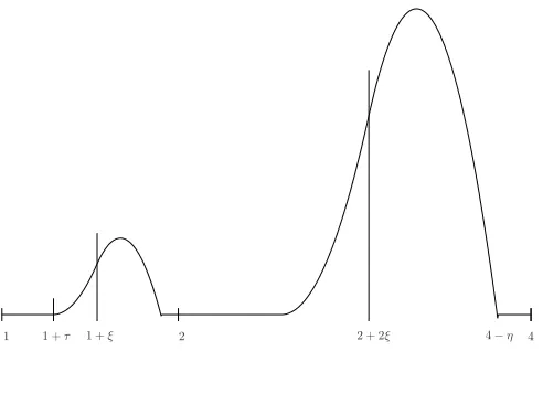
Lemma 4.2 (Existence ofQ). There exist parametersτ >0,ξ >0, and α >0 such that the solutionQto (3) on]1,4[, with a right-hand side defined by F (see (7)), and which is such thatQ≡0on ]1,1 +τ] andQ >0 in the right neighbourhood of 1 +τ, verifies the set of assumptions (8).
Proof. We fix α = 1.8, ξ = 0.54, and we denote by Qi the solution associated to the triplet of parameters (τi, α, ξ), withτ1= 0.29 andτ2= 0.30. With obvious notations, it can be established with the help of numerical
1 1 +τ 1 +ξ 2 2 + 2ξ 4−η 4
Figure 3. Function Q.
negative. By continuity, there exists a value τ ∈]0.29,0.30[ such that the identityβ+αη−4τ = 0 holds true for the solution associated to the triplet of parameters (τ, α, ξ). The shape of this solution is represented in
Fig.3.
Remark 4.3. The two solutions we built are obviously indistinguishable: asq1(2t) = 4q2(t), one cannot expect
any entropy-like criterium to be able to select between both.
5.
Extensions of the model
We end this paper with some comments on the possible extensions of this model. The first point we address here is a straightforward generalization of the convergence result. The other points are more prospective, and have not undergone a proper mathematical treatment.
5.1.
Alternative lubrication models
The approach we propose can be extended straighforwardly to the more general setting :
¨
qε=−ε qε˙
ϕ(qε)+f(t), (10)
whereq7−→ϕ(q)>0 is such thatφ(q) = Z 1
q
1
ϕ→+∞asq−→0.
In case the latter integral is convergent, contacts may occur, which makes our approach inappropriate. In case the integral is divergent, definingγε=εφ(qε), we get as in Theorem2.1convergence of (qε, γε) towards (q, γ), solution to (3). This extension covers the two-dimensionnal lubrication model (particles are in fact parallel cylinders), for which ϕ(q) =q−3/2(see [7]).
5.2.
Collisions
All this approach is based on the lubrication model (1), according to which the rigid body never touches the wall (see proposition1.1). It is common knowledge, though, that in many situations, contacts actually occur. Some factors may explain this discrepancy, and among them:
(1) bodies and walls are not smooth (smoothness is an essential assumption to establish the model (1)), they present a certain roughness which rules out the lubrication model when the distance gets too small; (2) as the distance drops below some threshold value, the Stokes model, which is based on a continuous medium assumption, is no longer valid, and alternative models, which may make contacts possible, must be considered.
We propose a heuristic way to integrate the fact that contact may actually occur, which suppresses the memory effects as the distance drops below a certain value. We introduce a threshold valueγ0, and we add in the model
the fact thatγis not allowed to go belowγ0.
Let us now describe the way we plan to use this approach to model real situations. Considering a fluid with finite viscosity ε >0, and surfaces with roughness e, we consider that the model is valid forq >2e, and that contact occurs as soon as q= 2e, which sets the value γ0 at εln(2e). Note that, from the numerical point of
view, this new model is quite easy to implement by simply introducing a cut-off ofγ atγ0.
5.3.
PDE version of this approach
We would like to finish with some comments on what might be a continuous-eulerian version of what we did at the discrete-lagrangian level. In [8] we proposed a macroscopic model to represent the global behaviour of an array of spherical particles interacting through lubrication forces. Denoting byρthe macroscopic density of the solid phase (ρ= 1 when all spheres are in contact), the inertial version of the model we propose reads
∂tρ+∂x(ρu) = 0
∂t(ρu) +∂x(ρu2)−∂x ε
1−ρ∂xu
= f
It is expected that a positive viscosityε, as small as it may be, prevents the densityρto go above the saturation value 1. Asεgoes to 0, one can expect the system to behave like a pressureless gas with a unilateral constraint
ρ≤1 (see [3,4]). Yet, as suggested by the present work, the limit behaviour is likely to exhibit a memory effect. It calls for the use of an extra variable, sayγ=γ(x, t), which can be expected to interact with the macroscopic velocityuin the following way:
∂tρ+∂x(ρu) = 0
∂t(ρu) +∂x(ρu2) +∂xp = f
∂tγ+∂x(γu) = −p γ≤0, ρ≤1, γ(1−ρ) = 0
wherepis an unknown pressure-like field which may take negative values (which distinguishes this gluey model from the standard pressureless gas situation), and γ is a field which keeps track of the constraint history experienced by a “fluid” particle, thus conveying its gluey character (note that ρis stuck to 1 as long as γ is negative). Like for pressureless gases, such a system must be provided with a collision law. Without it, nothing prevents two saturated blocks (ρ= 1) to collide in an elastic shock, with a restitution coefficient which may take any nonnegative value. This collision law may be defined by prescribing that, at any time, the right velocity
u+ is theL2-projection of the left velocityu−
onto the closure inL2 of
Cργ =
6.
Concluding remarks
We presented a framework to model the near-contact behaviour of a rigid body and a wall, under the asumption that the interstitial gap remains filled with a viscous fluid. The approach we presented is quite straightforward from the mathematical standpoint. Yet, it raises some issues regarding modelling. We would like to conclude by addressing the most paradoxal among them. As indicated by numerical computations (see Remark 3.1), reasonably small values for εlead to values for the interstitial gap which are much smaller than atomistic distances, and a fortiori much smaller than usual roughness parameters. From a modelling standpoint, it clearly invalidates this model in the case of small viscosity, in accordance with common sense: a rigid ball projected onto a clean wall does not stick to it, although air may be considered in many situations as a viscous fluid. As the limit model is obtained by letting the viscosity go to 0, one may wonder whether the limit model corresponds to any reality. Our belief (which has to be conforted by further analysis and experimental validation) is that, in a paradoxal way, this vanishing-viscosity model can be expected to have some validity in situations where the viscosity is large. Consider a physical situation, characterized by a given forcing termf, a threshold valueqlimbelow which the lubrication model (1) does no longer hold (typicallyqlimis linked with
the roughness of the surfaces), and a viscosityε. If the viscosity is small in such a way that lubrication forces (as given by model (1)) become significant for values ofqsmaller thanqlim, then our approach does not make
sense. On the contrary, if ε is large, one can expect q to remain above qlim, and the physical reality can be
expected to exhibit the gluey behaviour we described.
References
[1] P. Ballard,The Dynamics of Discrete Mechanical Systems with Perfect Unilateral Constraints, Arch. Rational Mech. Anal. 154, p.p. 199–274, 2000.
[2] I. Bazhlekov, F.N. van de Vosse, A.K.Chesters,Drainage and rupture of a newtonian film between two power-law liquid drops interacting under a constant force, J. Non-Newtonian Fluid Mech.,93, 181-201, 2000.
[3] F. Berthelin, Existence and weak stability for a pressureless model with unilateral constraint, Math. Models Methods Appl. Sci.,12, No 2, pp. 249–272, 2002.
[4] Y. Brenier, E. Grenier, Sticky particles and scalar conservation laws, SIAM J. Numer. Anal., 35, No 6, pp. 2317–2328 (electronic), 1998.
[5] Brenner,The slow motion of a sphere through a viscous fluid towards a plane surface, Chemical Engineering Science,16, pp. 242–251, 1961.
[6] S. Dharmatti and M. A. Ramaswamy,Hybrid control systems and viscosity solutions, J SIAM J. Control Optim.,44, No 4, pp. 1259–1288 (electronic), 2005.
[7] S. Kim and S. J. Karrila,Microhydrodynamics: Principles and Selected Applications, Butterworth-Heinemann, Boston, 1991. [8] A. Lefebvre, B. Maury,Micro-macro modelling of arrays of spheres interacting through lubrication forces, Pr´epublication du
Laboratoire de Math´ematiques de l’Universit´e Paris-Sud 2005-46.
[9] B. Maury,A Many-Body Lubrication Model, C. R. Acad. Sci. Paris, t.325, S´erie I, pp. 1053–1058, 1997.
[10] B. Maury,A time-stepping scheme for inelastic collisions, Numerische Mathematik, Volume 102, Number 4, pp. 649 - 679, 2006
[11] M. Schatzmann,A class of Nonlinear Differential Equations of Second Order in Time, Nonlinear Analysis, Theory, Methods & Applications,2, pp. 355–373, 1978.