Journal of Computing and Security
Solution of the Generalized Interval Linear Programming Problems:
Pessimistic and Optimistic Approaches
Mehdi Ghatee
a,∗
aDepartment of Computer Science, Amirkabir University of Technolog, Tehran, Iran.
A R T I C L E I N F O.
Article history:
Received:26 December 2012
Revised:12 February 2014
Accepted:28 June 2014
Published Online:13 September 2014
Keywords:
Interval Field, Interval Linear Programming, Total Ordering, Ranking Functions.
A B S T R A C T
This paper deals with linear programming problem with interval numbers as coefficients to exhibit with uncertainty. Since, the set of common intervals is not a field, we define generalized interval numbers to produce an algebraic interval field and on this field, we proposeprinciple of uncertainty traverse
instead of extension principlewhich permits to define operators on intervals exactly similar to the same operators on real numbers. In addition, we apply a total order on this field to transform interval linear programming into a traditional problem. The proposed order can be extended either pessimistically or optimistically. The numerical experiments are given to demonstrate the efficiency of the proposed scheme in comparison with the previous established works. The approach in this paper can be generalized to fuzzy linear programming problems taking the fuzzy cuts into account.
c
2014 JComSec. All rights reserved.
1
Introduction
For some considerable time, linear programming (LP) has been one of the operational research techniques, which has been widely used and got many achieve-ments in both applications and theories [1]. However the strict requirement of LP is that the data must be well defined and precise, which is often impossi-ble in real decision proimpossi-blems. The traditional way to evaluate any imprecision in the parameters of an LP model is through a post-optimization analysis, with the help of sensitivity analysis and parametric pro-gramming. However, none of these methods is suitable for an overall analysis of the effects of imprecision in parameters. Another way to handle impreciseness is to model it in stochastic programming problems ac-cording to the probability theory. A third way to cope with imprecision is to resort to the theory of interval
∗ Corresponding author.
No. 424, Hafez Avenue, Tehran, 15875-4413, Iran. Email address:[email protected](M. Ghatee) ISSN: 2322-4460 c2014 JComSec. All rights reserved.
mathematics or fuzzy sets, which give the conceptual and theoretical framework for dealing with complexity and uncertainty [2,3]. Interval mathematics started in 1950s and came more applicable in programming soon. They can handle uncertainty aspects accord-ing to the statistical analysis which can estimate the quantities bounds. Nowadays very researchers focus on this type of programming, see [4–6]. Also, intervals can be considered in fuzzy optimization when fuzzy cuts are followed [3,7,8]. Interval numbers are also important in numerical analysis, see e.g., [4,9–12].
numbers. In their work membership functions were defined as complex valued functions.
In parallel to these extensions, Kandel et al. [16] and Friedman et al. [17] in solving fuzzy linear systems found some contradiction solutions whose their right limits are less than their left limits. This contradiction is appeared from a gap in fuzzy numbers. Respect to the practitioners’ attempt for finding appropriate so-lutions to every system, Friedman et al. [17] accepted these unrealistic solutions and named them as weak fuzzy solutions. Allahviranloo [18] used this terminol-ogy, too. Chang and Lee [19] mentioned to the same problem in fuzzy regression and they proposed fuzzy numbers with spreads unrestricted in sign.
We believe that this gap in fuzzy numbers is a re-sult of similar gap in intervals. So we must fill the set of intervals with new numbers at first, which simplify the calculations. Our approach is to define arithmetic operators on interval numbers applying Ganesan and Veeramani’s approach [6]. For this aim, we propose a new appearance process of negative integers and we extend the operators in complex intervals to this new interval set to find a new definition for addition, mul-tiplication, subtraction and division. We show that the produced set with such operators is an algebraic field. For demonstrating the efficiency of this scheme, we argue linear programming on this interval field and we try to solve this problem with optimistic and pessimistic ranking functions [8,20]. In ordering cate-gory, Moore [21] is the first author which combined the previews results on0<0on real line and0⊆0on the
sets, to create two transitive order relations over inter-vals. Then, Ishibuchi and Tanaka [22] suggested two order relations≤LR and≤M W. However these
order-ing were not total order. Kundu [23] defined a fuzzy preference relationship between two interval and used it to find optimal decision. More differently Sengupta and Pal [8] suggested two index for comparing two intervals numerically. But these approaches focus on the lower and upper bound of intervals. In this paper we follow Hashemi et al.’ idea [3] for minimum interval cost flow problem. This approach provides a platform to take the risk into account. We show the efficiency of this approach for interval linear programming in this paper.
The rest of this paper is organized as follows: In Section2, we review on the classical theory of arith-metic operators on intervals and we discuss on some drawbacks. In Section3we introduce a generalization of intervals which produces a field of intervals. Then a total order by pessimistically and optimistically be-haviors is introduced. An interval linear programming with three groups of assumptions are solved in Sec-tion4. We also gave an application of the approach in
Section5. Section6ends the paper with conclusion and future directions.
2
Interval Numbers
An interval numberA= [aL, aR] is the set of all real
numbersx, such thataL≤x≤aR. We denote the set
of interval numbers byIN. IfaL=aR, thenAis a real
number or a degenerate. Interval.Ais alternatively represented asA=ha, αi, wherea= aL+aR
2 andα=
aR−aL
2 are center and width of interval number A, respectively. In this paper, we use the latter notation for representation of interval numbers. An interval
A=ha, αiis said to be nonnegative ifa−α≥0 and nonpositive ifa+α≤0.
Traditionally, arithmetic operations on interval numbers are defined by the extension principle [4,9]. Letf :< × < :→ <be a binary operation over real numbers. Then it can be extended to the operation over interval numbers. LetAandB be two interval numbers and∗ ∈ {+,−, ., /}be a binary operation on the set of real numbers, based on the extension prin-ciple, the binary operation∗over interval numbersA
andB can be defined as follows [9]:
A∗B={a∗b|a∈A, b∈B}. (1) In the case of division it is assumed that 0 not exists inB.
Thus forA=ha, αiandB =hb, βi, the extended addition, subtraction, multiplication, and division are derived as
ha, αi+hb, βi=ha+b, α+βi, (2)
ha, αi − hb, βi=ha−b, α+βi, (3)
ha, αi × hb, βi=h(d+c)/2,(d−c)/2i, (4)
ha, αi/hb, βi=h(f+e)/2,hf −e)/2i, (5) where
c= min{(a−α)(b−β),(a−α)(b+β),(a+α)(b−β),
(a+α)(b+β)},
d= max{(a−α)(b−β),(a−α)(b+β),(a+α)(b−β)
,(a+α)(b+β)}, e= min{a−α
b−β, a−α b+β,
a+α b−β,
a+α b+β}, f = max{a−α
b−β, a−α b+β,
a+α b−β,
a+α b+β}.
ha, αi × hb, βi=hab+αβ, aβ+bαi, (6)
ha, αi/hb, βi=hab+αβ
b2−β2,
aβ+bα
b2−β2i. (7) The extended interval operations2-5have been used in solving interval linear system of equations e.g. in Gaussian Elimination [10] and interval interpolation [4, 12]. However these operations cannot produce interval group and field.
Definition 1. A group is a set G which is closed under a binary operation ∗ (that is, for any x, y ∈
G, x∗y∈G) and satisfies the following properties: (1) Identity: There is an elemente∈G, such that
for everyx∈G, e∗x=x∗e=x.
(2) Inverse: For every x ∈ G there is an element
y ∈Gsuch thatx∗y=y∗x=e,where again e is the identity.
(3) Associativity: The following identity holds for everyx, y, z∈G:x∗(y∗z) = (x∗y)∗z. Definition 2. A group is said to be abelian ifx∗y=
y∗xfor everyx, y∈G.
Definition 3. A field is a setFwhich is closed under two binary operations + and ∗ (called addition and multiplication) such that
(1) F is an abelian group under + and
(2) F−{0}(the setFwithout the additive identity 0) is an abelian group under∗.
(3) For eachx, y, z∈F we have:
x∗(y+z) =x∗y+x∗z.
The identity elements under addition and multipli-cation operations are called zero and unit elements, respectively.
It is clear that the intervalh0,0iis the zero element for IN, but there is no addition inverse for interval numbers with positive width. Therefore, the set of in-terval numbers under binary operation2is not a group. Therefore, the setIN under binary operations2and 4as addition and multiplication operators is not a field. So we cannot solve system of interval equations efficiently. For example, we consider the simple exam-ple presented by Hansen [4]. Assume thatnintervals
Ai, i= 1, . . . , nare given and for eachi= 1, . . . , nwe
want the sum of all except theithinterval. Suppose
that we first compute the sum
S1=A2+. . .+An.
Afterwards, we want the sum
S2=A1+A3+. . .+An.
Instead of calculation the sum S2 directly, we are going to use subtraction formula 3. Note thatS2 =
S1+A1−A2. So we can computeS2by addingA1toS1 and then cancelingA2from the result by subtraction. ButA2−A2 =ha2−a2, α2+α2i=h0,2α2iis not the (degenerate) zero interval. Therefore, we cannot cancelA2fromS1 simply by subtracting unlessA2is real numbers.
Instead of subtracting using extended interval sub-traction, Hansen [4] used the special cancellation rule as follows:
ha, αi\hb, βi=ha−b, α−βi. (8) This operator is similar as Hukuhara’s difference for fuzzy numbers [24,25].
Now let us consider the following simple interval linear equation.
h35,2.5i+hx, yi=h50,3.5i. (9) In order to solve Equation9, we may write the follow-ing relation
hx, yi=h50,3.5i − h35,2.5i=h15,6i,
while this solution don’t satisfy in the Equation9. But if instead of extended subtraction we use the cancella-tion rule8, then we obtain the desired solutionh15,1i. Therefore, cancellation is more applicable in these cases in comparison with extended interval subtrac-tion. Now consider the interval numbersA=h150,10i
andB =h125,5i. Using cancellation rule8to compute
A\B, we obtainh25,−5i. Note thath25,−5iis not an interval number since the width of interval numbers must be nonnegative. So cancellation rule is not
3
Generalized Interval Numbers
As emphasized before, the set of interval numbers under binary operations2and4as addition and mul-tiplication operators is not a field and also it is not closed under cancellation rule. Our aim is to construct an algebraic field of intervals applying cancellation rule to define additive inverse. Here we allow interval numbers to take negative widths, and construct a new set of generalized interval as follows:
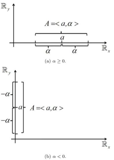
Definition 4. LetRx = {(x,0) ∈ R2|x ∈ R} and Ry={(0, y)∈R2|y∈R}. Generalized interval
num-berA=ha, αiis a convex closed subset of the union
Rxand Ry such that ifα ≥0, ha, αiis an ordinary
interval onRx and if α < 0 theha,−αi is an
ordi-nary interval onRy.The set of all generalized interval
numbers is denoted byGIN(R).
Figures1aand1bdepict the generalized intervalA
whenα≥0 andα <0,respectively.
(a)α≥0.
(b)α <0.
Figure 1. The representation of the generalized interval
A=ha, αi
the addition and multiplication ofAandB we have:
A+B=ha+b, α+βi. (10)
A×B =ha, αi × hb, βi=hab+αβ, aβ+bαi. (11) Then we can obtain directly:
−ha, αi=h−1,0i × ha, αi=h−a+ 0,0 + (−1)αi
=h−a,−αi. (12)
Thus the subtraction can be defined with the following:
A−B=A+ (−B) =ha−b, α−βi. (13) which is the same as cancellations rule8for ordinary intervals.
An intervalA=ha, αi,can be coupled with a tra-verse functionfA: [0, T]7→ ha.αisuch that
• T ≥0 is a decision period time.
• fAis one-to-one and continuous function. • fA(0) =a−αandfA(T) =a+α.
Then in addition and subtraction10and13,0+0and
0−0 operate on locations given by traverse functions fA(t) andfB(t) point-by-point wheretincreases from
0 up toT,i.e.
fA±B(t) =fA(t)±fB(t), ∀t∈[0, T].
Therefore whenB =A,sine fB(t) =fA(t) for each
t∈[0, T] we haveA−B= 0,or equivalentlyA−A= 0.
On the other hand, ifA, B≥0 we can write:
fA×B(0) =ab+αβ−(aβ+bα) = (a−α)(b−β)
=fA(0)×fB(0),
fA×B(T) =ab+αβ+ (aβ+bα) = (a+α)(b+β)
=fA(T)×fB(T),
thus again, we can write:
fA×B(t) =fA(t)×fB(t), ∀t∈[0, T].
These traverse functions are important, when uncer-tainty streams from pessimistically to the optimisti-cally statuses. In these cases, the level of uncertainty in data varies monotonically and with the same trend, the corresponding traverse functions change. We name this trend as principle of uncertainty traverse.
For introducing the inverse of intervalA=ha, αi
where |a| 6= |α|, by solving an easy mathematical exercise we obtain:
ha, αi × h a
a2−α2,
−α
a2−α2i=h1,0i= 1. We denote the inverse ofAwithA−1.If|a|=|α|,the inverse ofAis not well defined, because in these cases one of the bounds ofAis zero and divide on zero is not defined.
Now for division we can define:
A/B=A×B−1=ha, αi/hb, βi−1
=hab−αβ
b2−β2,
bα−aβ
b2−β2i, (14) where|b| 6=|β|.
It is clear that the set of generalized interval numbers is closed under binary operations 10 and 11. The following Proposition is the main result.
Proposition 1. The set of generalized interval num-bers under the binary operators10and11as addition and multiplication, is a field.
Proof. The set of generalized interval numbers is an abelian group under 10 with zero element h0,0i
and addition inverseh−a,−αifor generalized inter-valha, αi. Moreover,GIN(R)− {ha, αi}|a|6=|α| is an
abelian group under11with unit elementh1,0iand multiplication inverseha, αi−1=h a
a2−α2, −α a2−α2i.
Therefore we obtained an interval field as a frame-work for solving real problems.
[20] in which a ranking functionR:F(R)→Rthat
maps each interval number into the real line is defined for ordering the intervals. Thus by a natural order on real numbers we can compare interval numbers easily as follows:
A≥R B if and only ifR(A)≥R(B), A >R B if and only ifR(A)>R(B), A=R Bif and only ifR(A) =R(B).
We argue this approach in this article and use a modification of Hashemi et al.’ idea [3] which can treat with intervals pessimistically as well as optimistically. For this aim we give the following definition.
Definition 5. LetA=ha, αiandB=hb, βibe two given intervals. For each couple real positive numbers (k, l), less than or equal relation ≤k,l is defined as
following:
ha, αi ≤k,lhb, βi,
if and only if
k.(a−α) +l.(a+α)≤k.(b−β) +l.(b+β),
where≤means the common total order on real num-bersR.
Property 1. In the ordering definition 5, two im-portant parameterskandlare the importance of the center and the spread of interval in comparison pro-cess, respectively.
This property, easily, permit us to model risk averse, risk neutral, and risk seeking decision makers [3].
Proposition 2. Order relation≤k,lon interval
num-bers is a reflexive and transitive relation.
Corollary 1. The order in definition5can be defined applying the following linear ranking function:
R:GIN(R)7→R
R(ha, αi) =k.(a−α) +l.(a+α),
Therefore, this order belongs to the class of ranking function orders [20].
This order is not a total order. For providing this property, Hashemi et al. [3] limited the choice ofkand
l using non-algebraic numbers [26]. For example the ratio of circle circumference to its diameter denoted withπ'3.1415 and the base of the natural logarithm (e'2.7182) are non-algebraic. We have the following important result.
Proposition 3. Consider a non-algebraic real positive numberϑ. Let
k=q1ϑn1,
l=q2ϑn2,
where q1, q2 are two positive rational numbers and
n16=n2are nonnegative integer numbers. Then≤k,l
onTQ={ha, αi|a, α∈Q}is a total order.
Proof. See Proposition (2.8) in Hashemi et al. [3].
Property 2. Let A = ha, αi and B = hb, βi be in TQ,then
A=B, (15)
if and only if
k.(a−α) +l.(a+α) =k.(b−β) +l.(b+β), (16) if and only if
a=b, α=β, (17)
where k and l satisfy the assumptions of Proposi-tion3.
4
Interval linear programming
In this section we consider three interval models:
• Linear programming with interval cost function and real variables.
• Linear programming with interval coefficients and real variables.
• Linear programming with interval coefficients and variables.
We show the efficiency of our scheme in solving the corresponding linear programs in comparison with the following previous works on interval numbers:
• Pessimistic order relation.
ApessB iff a+α≤b−β (18) • Optimistic order relation.
AoptB iff a−α≤b+β (19) • Adamo’s order relation. [27]
AAOB iff a+α≤b+β (20) • Ishibuchi and Tanaka’s order relation [22].
ALRB iff a−α≤b−β
and a+α≤b+β, (a)
Amw B iff a≤b
and α≥β, (b)
(21)
4.1 LP with interval cost function
We present the following example to reveal the ef-ficiency of our scheme. The behind idea of this dis-cussion is tested by Hashemi et al. [3] on a special example of network flow problems.
Table 1. The optimal solution of Example1applying the proposed approach for some settings of (k, l).
(k, l) x1 x2 x3 x4 x5 x6 Optimal Value (1,100π) 0 0 166.67 0 0 200.00h2666.67,366.67i
(100π,1) 180.00 20.00 0 0 120.00 0 h920.00,1500.00i
(π/2,1) 0 200.00 100.00 0 0 0 h1200.00,700.00i
(π/7,1) 200.00 0 166.67 0 0 0 h1466.67,566.67i
(π/19,1) 0 0 166.67 0 0 200.00h2666.67,366.67i
min h4,2ix1+h4,3ix2+h4,1ix3+h6,5ix4 +h1,9ix5+h10,1ix6,
(22)
s.t.
x1+x2+x4+x6≥200,
x1+ 3x3+x5≥300,
x2+ 3x3−x4+ 4x5≥500,
x1, ..., x6≥0.
The result for five couple of (k, l) by our approach is presented in Table1.
This table shows that the effect of increasing in the values of k or l, is similar. Thus choosing the appropriate values for these parameters is not very hard work. Also, Table1illustrates that for a fixed
l= 1 the center of optimal values strictly increases by decreasing the value ofk.
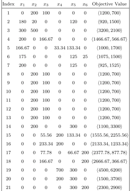
In addition, all of the feasible extreme points of this problem and their corresponding objective values are mentioned in Table2.
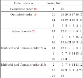
For comparing the results, we sort the extreme solutions of problem based on different ordering. For this aim, for each ordering, we give a list of indices of solutions such as{t1, ..., tN}(N is not necessarily
equal to the number of solutions) such that for each
i= 1, ..., N−1,the objective value of (ti)thsolution
is less than the objective value of (ti+1)th solution
based on the considered order. In Table3, pessimistic order18, optimistic order19, Adamo’s order20and finally Ishibuchi and Tanaka’s orders21.a and 21.b are compared. As you see, the possibility of inserting a solution in the list depends on the previous inserted solution. This causes to consider only solutions which can be compared together.
Table3reveals that our proposed scheme can find solutions similar to other ordering when the impor-tance weightskandlare changed. Also the pessimistic order18and Ishibuchi and Tanakas’ order21.a and 21.b cannot rank solutions totally, which is a drawback of these methods. However the results of Adamo’s order20is similar to the Ishibuchi and Tanakas’
or-Table 2. The feasible extreme solutions (points) of Example1 and their objective values.
Index x1 x2 x3 x4 x5 x6 Objective Value
1 0 200 100 0 0 0 h1200,700i
2 180 20 0 0 120 0 h920,1500i
3 300 500 0 0 0 0 h3200,2100i
4 200 0 166.67 0 0 0 h1466.67,566.67i
5 166.67 0 0 33.34 133.34 0 h1000,1700i
6 175 0 0 0 125 25 h1075,1500i
7 200 0 0 0 125 0 h925,1525i
8 0 200 100 0 0 0 h1200,700i
9 0 200 100 0 0 0 h1200,700i
10 0 200 100 0 0 0 h1200,700i
11 0 200 100 0 0 0 h1200,700i
12 0 200 100 0 0 0 h1200,700i
13 0 200 100 0 0 0 h1200,700i
14 0 200 0 0 300 0 h1100,3300i
15 0 0 55.56 200 133.34 0 h1555.56,2255.56i
16 0 0 233.34 200 0 0 h2133.34,1233.34i
17 0 0 77.78 0 66.67 200 h2377.78,877.78i
18 0 0 166.67 0 0 200 h2666.67,366.67i
19 0 0 0 700 300 0 h4500,6200i
20 0 0 0 200 300 0 h1500,3700i
21 0 0 0 0 300 200 h2300,2900i
der21.a in the starting indices of solution lists (index 1 to 8) and all of them are predicted by our scheme, fortunately.
4.2 LP with interval coefficients and real vari-ables
In this subsection, we generalize the Example1, by some new assumptions to present the new concept of the efficiency of the proposed scheme.
Table 3. The sorted list of extreme solutions applying different orders18,19,20and21
Order relation Sorted list
Pessimistic order18 1 18
Optimistic order19 21 20 19 18 17 16 15 14 13 12 11 10 9 8
7 6 5 4 3 2 1
Adamo’s order20 13 12 11 10 9 8 1 4 2 7 6 5 18 17 16 15 14 21 20 3 19 Ishibuchi and Tanaka’s order21.a 13 12 11 10 9 8 1
4 5 7 6 14 15 16
20 21 3
Ishibuchi and Tanaka’s order21.b 2 5 7 6 14 13 12 11 10 9 8 1 4 20
21 18
min h4,2ix1+h4,3ix2+h4,1ix3+h6,5ix4 +h1,9ix5+h10,1ix6,
(23)
s.t.
h1,0.5ix1+h1,1ix2+x4+x6≥ h200,10i,
h2,1ix1+h3,2ix3+x5≥ h300,50i,
h1,1ix2+h3,2ix3− h2,1ix4+h4,3ix5≥ h500,40i,
x1, ..., x6≥0.
The constraints of this problem may be rewritten as follows:
hx1+x2+x4+x6,0.5x1+x2i ≥ h200,10i,
h2x1+ 3x3+x5, x1+ 2x3i ≥ h500,40i,
hx2+ 3x3−2x4+ 4x5, x2+ 2x3−x4+ 3x5i
≥ h500,40i,
or by utilizing our ordering5with some fixed couples of (k, l) satisfying in Proposition3, we have
(k+ 0.5l)x1+ (k+l)x2+kx4+kx6
≥200k+ 10l,
(2k+l)x1+ (3k+ 2l)x3+kx5
≥500k+ 40l,
(k+l)x2+ (3k+ 2l)x3−(2k+l)x4+ (4k+ 3l)x5
≥500k+ 40l,
Therefore this case is transformed to the previous case which is presented in Example1.
4.3 LP with interval coefficients and vari-ables
In the bellow, a fully interval version of linear pro-gramming is introduced. This model can handle the uncertainty concepts in framework of problem and in decision maker’s solutions.
Example 3. Consider the following interval problem with interval variables:
min h4,2i×hx1, ξ1i+h4,3i×hx2, ξ2i+h4,1i×hx3, ξ3i
+h6,5i × hx4, ξ4i+h1,9i × hx5, ξ5i+h10,1i × hx6, ξ6i, (24) s.t.
h1,0.5i×hx1, ξ1i+h1,1i×hx2, ξ2i+x4+x6≥ h200,10i,
h2,1i × hx1, ξ1i+h3,2i × hx3, ξ3i+x5≥ h300,50i,
h1,1i × hx2, ξ2i+h3,2i × hx3, ξ3i − h2,1i × hx4, ξ4i +h4,3i × hx5, ξ5i ≥ h500,40i,
x1−ξ1, ..., x6−ξ6≥0.
By arithmetic operators10 and11, this problem simplifies as follows:
+6ξ4+ 9x5+ξ5+x6+ 10ξ6i, (25) s.t.
hx1+ 0.5ξ1+x2+ξ2+x4+x6,0.5x1+ξ1 +x2+ξ2i ≥ h200,10i
h2x1+ξ1+ 3x3+ 2ξ3+x5, x1+ 2ξ1+ 2x3 +3ξ3i ≥ h300,50i,
hx2+ξ2+ 3x3+ 2ξ3−2x4−ξ4+ 4x5+ 3ξ5, x2+
ξ2+ 2x3+ 3ξ3−x4−2ξ4+ 3x5+ 4ξ5i ≥ h500,40i, The objective function can be rewritten as bellow:
min h4,2ix1+h4,3ix2+h4,1ix3+h6,5ix4+h1,9ix5 +h10,1ix6+h2,4iξ1+h3,4iξ2+h1,4iξ3+h5,6iξ4
+h9,1iξ5+h1,10iξ6.
Also applying the ordering5with some fixed couples of (k, l) fulfilling in Proposition3, we can transform the constraint as follows:
(k+ 0.5l)x1+ (0.5k+l)ξ1+ (k+l)x2+ (k+l)ξ2 +kx4+kx6≥200k+ 10l
(2k+l)x1+ (k+ 2l)ξ1+ (3k+ 2l)x3+ (2k+ 3l)ξ3 +kx5≥300k+ 50l,
(k+l)x2+ (k+l)ξ2+ (3k+ 2l)x3+ (2k+ 3l)ξ3
−(2k+l)x4−(k+ 2l)ξ4+ (4k+ 3l)x5 +(3k+ 4l)ξ5≥500k+ 40l.
Thus a problem with interval objective function and real restriction is obtained and the result of Example1 is applicable for this state, too. Only note that this problem includes two series of variables.
4.4 LP with fuzzy numbers
A linear programming with fuzzy parameters can be used to model a real problem under uncertainty. Such models are very applicable for long-term decision making. Fuzzy optimization models can be solved differently. In [20], three different approaches for fuzzy ordering have been discussed which can be considered to produce algorithms for fuzzy optimization. Also each fuzzy number ˜A can be represented with its
α−cuts directly, see e.g., [7]. Then for a fixed certainty degree, it is possible to consider one of the α−cuts in which all of the members inα−cut corresponds a possibility degree greater thanα.Since theα−cut for a fuzzy number is an interval, all of the concepts given in the previous subsections are valid.
5
Application
Assume there are nprojects for investment. Let< ci, γi>is the profit ofithproject considering all of the
information and experiments. We need to maximize the following interval value objective function:
maxz=
n
X
i=1
< ci, γi> xi, (26)
where non-negative variablexiis the amount of capital
which is invested in projecti.
Let risk of investment inithproject is< r
i, αi> .If
the bound for risk is given by< ti, βi> .This dictate
to consider the following constraint:
n
X
i=1
< ri, αi > xi ≤ < ti, βi>, (27)
This problem needs to solve under the following budget restriction:
n
X
i=1
xi≤B, (28)
The approach of this paper can be followed to solve this uncertain problem.
6
Conclusion and future direction
References
[1] Y. Matsuo M. Ishizuka. Sl method for computing a near-optimal solution using linear and non-linear programming in cost-based hypothetical reasoning. Knowledge-Based Systems, 15:369– 376, 2002.
[2] T.K. Pal A. Sengupta. Solving the shortest path problem with interval arcs. Fuzzy Optimization and Decision Making, 5:79–99, 2006.
[3] E. Nasrabadi S.M. Hashemi, M. Ghatee. Combi-natorial algorithms for minimal interval cost flow problem.Applied Mathematics and Computation, 175:1200–1216, 2006.
[4] E. Hansen. Global Optimization Using Interval Analysis. Marcel Dekker Inc., USA, 1992. [5] O. Didrit L. Jaulin, M.Kieffer and E. Walter.
Ap-plied Interval Analysis. Springer, London, 2001. [6] P. Veeramani K. Ganesan. On arithmetic opera-tions of interval numbers. International Journal of Unccertainty, Fuzziness and Knowledge-Based Systems, 13:619 – 631, 2005.
[7] S.M. Hashemi M. Ghatee. Ranking function-based solutions of fully fuzzy minimal cost flow problem. Information Sciences, 177:4271–4294, 2007.
[8] T.K. Pal A. Sengupta. Theory and methodology on comparing interval numbers. European Jour-nal of OperatioJour-nal Research, 127:28–43, 2000. [9] R.E. Moore. Interval analysis. Prentice-Hall,
Englewood cliffs, New Jersey, 1969.
[10] E.R. Hansen. Interval forms of newton’s method.
Computing, 20:153–163, 1978.
[11] M. Novoa R.B. Kearfott and C. Hu. Precondition-ers for the interval gauss-seidel method. Interval Computations, 1:59–85, 1991.
[12] K. Nickel. Interval mathematics. In Proceed-ings of the International Symposium in Freiburg, Springer, Wien, pages 23–36, 1985.
[13] R.Boche. Complex interval arithmetic with some applications. Lockheed Missiles and Space Co, report 4-22-66-1, 1966.
[14] M.S. Petkovic and L.D. Petkovic. Complex Inter-val Arithmetic and Its Applications. John Wiley and Sons, 1998.
[15] M.Friedman D. Ramot, R.Milo and A. Kandel. Complex fuzzy sets.IEEE Transactions on Fuzzy Systems, 10:171–186, 2002.
[16] M. Friedman A.Kandel and M. Ming. Fuzzy linear systems and their solution. InIEEE International Conference on Systems, Man and Cybernetics,
volume 1, pages 336–338, 1996.
[17] A. Kandel M. Friedman, M. Ming. Fuzzy linear systems. Fuzzy Sets and Systems, 96:201–209, 1998.
[18] T. Allahviranloo. The adomian decomposition
method for fuzzy system of linear equations. Ap-plied Mathematics and Computation, 163:553– 563, 2005.
[19] E.S. Lee P.T. Chang. Fuzzy linear regression with spreads unrestricted in sign. Computers&
Mathematics with Applications, 28:61–70, 1994. [20] E. Kerre X. Wang. Reasonable properties for the
ordering of fuzzy quantities(i). Fuzzy Sets and Systems, 118:375–385, 2001.
[21] R.E. Moore. Method and application of interval analysis. SIAM, Philadelphia, 1979.
[22] H. Tanaka M. Ishibuchi. Multiobjective program-ming in optimization of the interval objective function. European Journal of Operational Re-search, 48:219–225, 1990.
[23] S. Kundu. Min-transitivity of fuzzy leftness rela-tionship and its application to decision making.
Fuzzy Sets and Systems, 86:357–367, 1997. [24] M. Hukuhara. Int´egration des applications
mea-surable dont la valeur est un compact convexe.
Funkc. Ekvacioj., 10:205–223, 1967.
[25] R. Korner P. Diamond. Extended fuzzy linear models and least squares estimates.Computers&
Mathematics with Applications, 33:15–32, 1997. [26] M. Filaseta. Algebric Number theory, Instructor
notes. University of South Carolina, 1999. [27] J.M. Adamo. Fuzzy decision trees. Fuzzy Sets
and Systems, 4:207–219, 1980.