An Interval Matrix Based Generalized Newton Method for Linear Complementarity Problems

http://dx.doi.org/10.4236/ojapps.2015.58044

An Interval Matrix Based Generalized

Newton Method for Linear

Complementarity Problems

Hai-Shan Han, Lan-Ying

College of Mathematics, Inner Mongolia University for the Nationalities, Tongliao, China Email: haishanhan@sohu.com

Received 6 July 2015; accepted 9 August 2015; published 12 August 2015

Copyright © 2015 by authors and Scientific Research Publishing Inc.

This work is licensed under the Creative Commons Attribution International License (CC BY).

http://creativecommons.org/licenses/by/4.0/

Abstract

The penalty equation of LCP is transformed into the absolute value equation, and then the exis-tence of solutions for the penalty equation is proved by the regularity of the interval matrix. We propose a generalized Newton method for solving the linear complementarity problem with the regular interval matrix based on the nonlinear penalized equation. Further, we prove that this method is convergent. Numerical experiments are presented to show that the generalized Newton method is effective.

Keywords

Linear Complementarity Problem, Nonlinear Penalized Equation, Interval Matrix, Generalized Newton Method

1. Introduction

The linear complementarity problem, denoted by LCP M q

(

,

)

, is to find a vector n

x∈R such that

(

)

T

0, 0, 0

There exist several methods for solving LCP M q

(

,

)

, such as projection method, multi splitting method, inte-rior point method, and the nonsmooth Newton method, smoothing Newton method, homotopy method etc. See

[1]-[6] and its references.

In [7], it given a nonlinear penalized Equation (1.2) corresponding to linear complementarity problem (1.1). Find x_λ∈Rn such that

[ ]

1

k

Mx_λ+λ x_{λ +} =q (1.2) where λ >1 is the penalized parameter, k>0,

[ ]

u ₊=max

{ }

u, 0 and yα =

(

y₁α,y₂α,,y_nα

)

T for any

(

)

T

1, 2, ,

n n

y= y y  y ∈R .

The nonlinear penalized problems (1.2) corresponding to the linear complementarity problem (1.1), which its research has achieved good results. In 1984, Glowinski [1] studied nonlinear penalized Equation (1.2) in Rn, and proved the convergence of penalized equation that matrix A was symmetric positive definite. In 2006, Wang et al. [8] presented a power penalty function approach to the linear complementarity problem arising from pricing American options. It is shown that the solution to the penalized equation converges to that of the linear complementarity problem with matrix is positive definite. In 2008, Yang [7] proved that solution to this pena-lized Equations (1.2) converged to that of the LCP at an exponential rate for a positive definite matrix case where the diagonal entries were positive and off-diagonal entries were not greater than zero. The same year, Wang and Huang [9] presented a penalty method for solving a complementarity problem involving a second- order nonlinear parabolic differential operator, and defined a nonlinear parabolic partial differential equation (PDE) approximating the variational inequality using a power penalty term with a penalty constant λ>1, a power parameter k >0 and a smoothing parameter ε. And prove that the solution to the penalized PDE con-verges to that of the variational inequality in an appropriate norm at an arbitrary exponential rate of the form

1/ 1/2 ([ k (1 k)] )

O λ− +ε +λε . Under some assumptions, Li [10] [11] proved that the solution to this equation con-verges to that of the linear complementarity problem with A is a strict row diagonally dominant upper trian-gular P-matrix when the penalty parameter approaches to infinity and the convergence rate was also exponential. It is worth mentioning that the penalty technique has been widely used solving nonlinear programming, but it seems that there is a limited study for the LCP.

Although the studies solving for the linear complementarity problem based on the nonlinear penalized equa-tion have good results. But there is no method that is given for solving the nonlinear penalized equaequa-tion. Throughout the paper, we propose a generalized Newton method for solving the nonlinear penalized equation with under the suppose

[

M M, +λI

]

is regular. So the method can better to solve linear complementarity problem. We will show that the proposed method is convergent. Numerical experiments are also given to show the effectiveness of the proposed method.

2. Preliminaries

Some words about our notation: I refers to the identity matrix, and ⋅ represents the 2-norm. For x∈Rn, all vectors are column vectors, xT refers to the transpose of the x,

[ ]

x₊ =max

{ }

x, 0 , that generalized Jaco-bian ∂

[ ]

x₊ =D x

( )

, where D x

( )

denotes diagonal matrix, On the diagonal elements with component 1.0 or

[ ]

0,1

σ∈ corresponding to the component of x which is positive , negative or zero, respectively.

The definition of interval matrix arises from the linear interval equations [12], given two matrices A=

( )

A_ij and A=

( )

A_ij , an interval matrix _AI ₌_{A A}, ₌

{

_{A A}: _{≤ ≤A A}

}

  , where A≤A refers to Aij ≤Aij for each ,

i j. AI is called regular if each A∈AI is nonsingular.

Lemma 1: Assume that interval matrix

[

M M, +λI

]

is regular. Then for diagonal matrix D x

( )

_λ and real number λ >1, M+λD x

( )

_λ is nonsingular.

[

,

]

M+λD∈ M M+λI

By the assumptions, we have M+λD x

( )

_λ is nonsingular. □ Lemma 2: Let x y, ∈Rn. Then

[ ] [ ]

x ₊− y₊ ≤ x−y

Definition 1 [1]: A matrix M∈Rn n× is said to be a P-matrix if all its principal minors are positive.

Lemma 3 [1]: A matrix M∈Rn n× is a P-matrix if and only if the LCP q M

(

,

)

has a unique solution for all vectors q∈Rn.

3. Generalized Newton Method

In this section, we will propose that a new generalized Newton method based on the nonlinear penalized equa-tion for solving the linear complementarity problem. Because when k>1, penalty term of the nonlinear pena-lized equation (1.2) is none Lipschitz continuously, hence we only discusses a case that k=1. So from nonli-near penalized equation (1.2), we have that

[ ]

Mx_λ+λ x_{λ +}=q (3.1) These case penalty problems for the continuous Variational Inequality and the linear complementarity prob-lems are discussed in [2] [13].

Let us note

( )

[ ]

, 1

f x_λ =Mx_λ+λ x_{λ +}−q λ> (3.2) Thus, nonlinear penalized equation (3.1) is equivalent to the equation f x

( )

λ =0.

A generalized Jacobian ∂f x

( )

_λ of f x

( )

_λ is given by

( )

( )

f xλ M λD xλ

∂ = +

where D x

( )

_λ = ∂

[ ]

x_{λ +} is a diagonal matrix whose diagonal entries are equal 1,0 or a real number σ∈

[ ]

0,1 depending on whether the corresponding component of x_λ is positive, negative, or zero. The generalized Newton method for finding a solution of the equation f x

( )

_λ =0 consists of the following iteration:

( )

( )(

1

)

0

i i i i

f xλ + ∂f xλ xλ+ −xλ = (3.3)

Then

( )

i i1

( )

i i

( )

i

f x_λ x_λ+ f x_λ x_λ f x_λ

∂ = ∂ −

( )

( )

( )

1

i i i i i i

k k k

i i i

k k

M D x x M D x x Mx x q

D x x x q

λ λ λ λ λ λ

λ λ λ

λ λ λ

λ λ

+

+

+

 

 +  = +  − +  _{ } −

     

 

= − _{ } +

Since D x

( )

_λi xi_λ =   xi_{λ +}, consequently

( )

i i1

k

M λ D x_λ x_λ+ q

 +  =

  (3.4) Proposition 1 Mx_λ+λ

[ ]

x_{λ +}=q equivalent to 0≤ ⊥z Az+ ≥b 0, where

(

)

1 1

, ,

z=Mxλ−q A= M+λI M− b=λM q−

Proof: Since 2 , 0

0, 0

x x

x x

x

λ λ

λ λ

λ

≥ 

+ =  _<

 , then

[ ]

(

)

1 2

[ ]

1

(

)

1 1

0

2 2 2

Mx_λ+λ x_{λ +}− =q Mx_λ+λ x_λ +x_λ − =q _M+λ I x_{ λ}+λ x_λ − =q

 

(

2M+λI x

)

_λ+λ x_λ −2q=0 By [14], its equivalent to

(

)

(

)

0≤ 2M+λI x_λ−λx_λ−2q⊥ 2M+λI x_λ+λx_λ−2q≥0

(

)

0≤Mx_λ− ⊥q M+λI x_λ− ≥q 0 (3.5) Let z=Mxλ−q then

(

M +λI x

)

λ− =q

(

M +λI M

)

−1

(

z+q

)

− =q

(

M +λI M z

)

−1 +λM q−1 . □

Proposition 2 Mxλ+λ

[ ]

xλ +=q has a unique solution if and only if the interval matrix

[

M M, +λI

]

is regular.

Proof: Since M M, +λI∈

[

M M, +λI

]

, by theorem 1.2 of [12], if

[

M M, +λI

]

is regular, then

(

)

1

M+λI M− is P-matrix, which implies that the LCP has a unique solution for any q∈Rn [1], from the re- lation between the (3.1) and the LCP (3.5), we can easily deduce that the (3.1) is uniquely solvable for any

n

q∈R . □ Algorithm 3

Step 1: Choose an arbitrary initial point 0

0 n

x_λ ∈R , ε >0 and given λ >0 1, µ>1, σ∈

[ ]

0,1 , let k: 0= ;

Step 2: for the λk, computer 1 k

i

xλ+ by solving

( )

1

k k

i i

k

M λ D x_λ x_λ+ b

 +  =

  (3.6) Step 3: If 1

k k

i i

xλ+ −xλ <ε, let k

i k

x =xλ go to step 4. Otherwise, i= +i 1 go to step 2.

Step4: If xk+1−xk <ε and Mxk− <q ε , terminate, x=xk is solution of LCP. Otherwise let

1

k k

λ+ =µλ , 1 0

k k

x_λ+ =x let k:= +k 1, go to 2.

4. The Convergence of the Algorithm

We will show that the sequence

{ }

1

k i

i x_λ ∞

= generated by the generalized Newton iteration (3.6) converges to an

accumulation point xk associated with λk. First, we establish boundness of the sequence

{ }

k i

xλ for any

0 k

λ > generated by the Newton iterates (3.6) and hence the existence of accumulation point at each genera-lized Newton iteration.

Theorem 3: Suppose that the interval matrix

[

M M, +λkI

]

is regular. Then, the sequence

{ }

k i

x_λ generated by Algorithm 3 is bounded. Consequently, there exits an accumulation points xk such that

( )

k k k

M λ D x x b

 +  =

  .

Proof: Suppose that sequence

{ }

xi_λk is unbounded, Thus, there exists an infinite nonzero subsequence

{ }

j

{ }

k k

i i

x_λ ⊂ x_λ such that

{ }

j ,

( )

j and

[ ]

0,

k k

i i

x_λ → ∞ D x_λ =D D∈ I

where D is main diagonal element of diagonal matrix which is 1, 0,σ∈

[ ]

0,1 .

We know subsequence j k j k

i

i

x

x

λ

λ

 

 

 

 

 

is bounded. Hence, exists convergence subsequence and assume that

(

)

j k

j j

k k

i

k i i

x _b A D x x λ λ λ λ +  =

Letting j→ ∞ yields

(

M+λ_kD x 

)

=0, x =1.

Since M+λkD∈

[

M M, +λkI

]

and the interval matrix

[

M M, +λkI

]

is regular, we know that

(

)

1

k

M+λ D − is exists and hence x=0, contradicting to the fact that x =1. Consequently, the sequence

{ }

k

i

xλ is bounded and there exists an accumulation point xk of

{ }

k i

xλ such that

( )

(

)

1

k k k

x = M+λ D x − b □ Under a somewhat restrictive assumption we can establish finite termination of the generalized Newton itera-tion at a penalized equaitera-tion soluitera-tion as follows.

Theorem 4: Suppose that the interval matrix

[

M M, +λkI

]

is regular and

(

( )

)

1 ₁ 2 k i k k M λ D x_λ

λ

−

+ < holds

for all sufficiently large λ_k, then the generalized Newton iteration (3.6) linearly converges from any starting point 0

k

xλ to a solution xk of the nonlinear penalized equation (3.1).

Proof: Suppose that xk is a solution of nonlinear penalized equation. By the lemma 1, M+λkD x

( )

λk is nonsingular. To simply notation, let D=D x

( )

k ,

( )

k

i i

D =D x_λ and since

(

M+λ_kD x

( )

_k

)

x_k =b,

( )

1

k k

i i

k

M λ D x_λ x_λ+ b

 +  =

  have Dxk =

[ ]

xk +, k k i i i

D xλ =  xλ ₊, hence

(

)

(

[ ]

)

(

)

[ ]

(

)

[ ]

(

)

(

)

[ ]

(

)

(

)

(

)

1 1 1

1

1

1

k k k

k k k

k k k

k k k

i i i i i

k k k k k k

i i i i

k k

i i i i

k k k k k

i i i i i

k k k k k k

M x x D x b Dx b D x x

D x x x x

x x D x x x x

x x D x x D x x

λ λ λ

λ λ λ

λ λ λ

λ λ λ

λ λ λ

λ

λ λ

λ λ λ

+ + + + + + + + + + + + − = − + + − = − − = − − + −   = − _{ } − − − + −   = − _{ } − − − − −

(

)

(

1

)

(

[ ]

)

(

)

k k k

i i i i i

k k k k k k

M λ D x_λ+ x λ x_λ x ₊ λ D x x_λ

+

 

+ − = − _{ } − − −

(

₁

) (

)

1

(

(

[ ]

)

(

)

)

k k k

i i i i i

k k k k k k

x_λ+ x M λ D − λ x_λ x ₊ λ D x_λ x

+

 

− = + − _{ } − + −

since

(

( )

)

1 1 2 k

i k

k M λ D x_λ

λ

−

+ < and by the lemma 2, we have

(

)

(

)

(

(

)

)

(

)

(

) (

)

1 1 1 2 2 k k k k

i i i

k k k k

i i i

k k k k

x x M D x x

M D x x x x

λ λ λ λ λ λ λ λ − + − − ≤ + −

= ⋅ + − < −

(4.2)

Letting i→ ∞ and taking limits in both sides of the last inequality above, we have

(

)

(

)

1 1 k k i k i k x x x x λ λ + ₋ < −

So the iteration (3.6) linearly converges to a solution xk of nonlinear penalized equation (3.1). □ In here, we will focus on the convergence of Algorithm 3.

( )

(

)

1 ₁

2 k

i k

k M λ D x_λ

λ

−

+ < holds, then Algorithm 3 linearly converges from any starting point 0 0

xλ to a

solu-tion *

x of the LCP M q

(

,

)

(1.1).

Proof: Since M is P-Matrix, then the LCP M q

(

,

)

has a unique solution, let the solution denote *

x , by the assumptions of the theorem, the generalized Newton iteration (3.6) linearly converges to a solution xk of the nonlinear penalized equation (3.1).

1 1 1 1 1 1 1

* * *

k k k k k k k k k k k

i i i i i i i i

x_λ+ −x = x_λ+ −x_λ+ +x_λ+ −x_λ +x_λ −x ≤ x_λ+ −x_λ+ + x_λ+ −x_λ + x_λ −x

let i→ ∞, then

1 1

* *

k k k k

x_λ+ −x ≤ x_λ+ −x_λ + x_λ −x

we have 1 *

*

lim k 1

k

k

x x

x x

λ

λ +

→∞

− ≤

− □

5. Numerical Experiments

In this section, we give some numerical results in order to show the practical performance of Algorithm 2.1. Numerical results were obtained by using Matlab R2007 (b) on a 1G RAM, 1.86 Ghz Intel Core 2 processor. Throughout the computational experiments, the parameters were set as ε =1.0e−8, λ =0 10, µ=2.

Example 1: The matrix A of linear complementarity problem LCP A b

(

,

)

of as follows (This example appear in the Geiger and Kanzow [15], Jiang and Qi [16], YONG Long-quan, DENG Fang-an, CHEN Tao [17]):

(

)

T

4 1 0 0 0

1 4 1 0 0

0 1 4 0 0

, 1, 1, , 1, 1

0 0 0 4 1

0 0 0 1 4

A b

−

 

_{− −} 

 

 − 

=  = − − − −

 

 ₋ 

 

 ₋ 

 

  



     

 

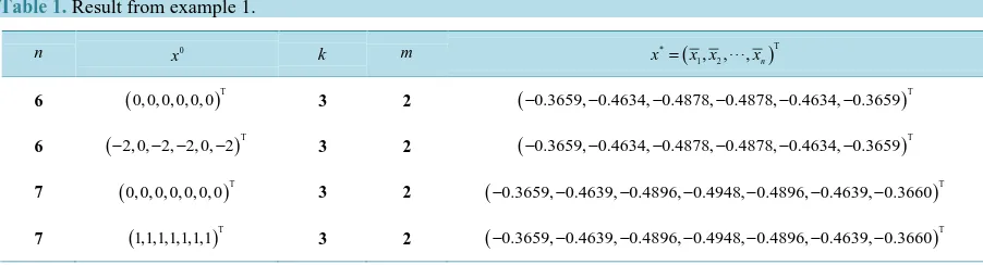
The computational results are shown in Table 1. This x0 is initial point, k is number of inner iterations, the outer iteration number is m, x* is iteration results.

Example 2: The matrix A of linear complementarity problem LCP A b

(

,

)

of as follows (This example appear in the Geiger and Kanzow [15], Jiang and Qi [16], YONG Long-quan, DENG Fang-an, CHEN Tao [17]):

(

)

T

1 2

diag , ,1 , 1, 1, 1, ,1, 1 ,

A b

n n

 

= _{ } = − − − −

   

The computational results are shown in Table 2. This 0

x is initial point, k is number of inner iterations, the outer iteration number is m, *

[image:6.595.87.538.597.719.2]

x is iteration results.

Table 1. Result from example 1.

n 0

x k m * ( )T

1, 2, , n

x = x x x

6 (0, 0, 0, 0, 0, 0)T 3 2 (−0.3659, 0.4634, 0.4878, 0.4878, 0.4634, 0.3659− − − − − )T

6 (−2, 0, 2, 2, 0, 2− − − )T 3 2 (−0.3659, 0.4634, 0.4878, 0.4878, 0.4634, 0.3659− − − − − )T

7 (0, 0, 0, 0, 0, 0, 0)T 3 2 (−0.3659, 0.4639, 0.4896, 0.4948, 0.4896, 0.4639, 0.3660− − − − − − )T

[image:7.595.95.539.81.231.2]

Table 2. Result from example 2.

n 0

x k m * ( )T

1, 2, , n

x = x x x 6 (1, 1,1, 1,1, 1− − −)T 3 2 (− − − −6, 3, 2, 1.5, 1.2, 1− −)T

6 (0, 0, 0, 0, 0, 0)T 3 2 (− − − −6, 3, 2, 1.5, 1.2, 1− −)T

8 (0, 0, 0, 0, 0, 0, 0, 0)T 3 2 (− − −8, 4, 2.67, 2, 1.6, 1.34, 1.14, 1− − − − −)T

8 (1, 1,1, 1,1, 1,1, 1− − − −)T 3 2 (− − −8, 4, 2.67, 2, 1.6, 1.34, 1.14, 1− − − − −)T

16 (1, 1,1, 1,− − ,1, 1− )T 3 2 (−16, 8, 5.3, 4, 3.2, 2.67, 2.28, 2, 1.78, 1.6, 1.45, 1.34, 1.23, 1.14, 1.06, 1− − − − − − − − − − − − − − − )T

16 (0, 0, 0, 0,, 0, 0)T 3 2 (−16, 8, 5.3, 4, 3.2, 2.67, 2.28, 2, 1.78, 1.6, 1.45, 1.34, 1.23, 1.14, 1.06, 1− − − − − − − − − − − − − − − )T

Supported

This work supported by the Science Foundation of Inner Mongolia in China (2011MS0114)

References

[1] Cottle, R.W., Pang, J.-S. and Stone, R.E. (1992) The Linear Complementarity Problem. Academic Press, San Diego [2] Glowinski, R. (1984) Numerical Methods for Nonlinear Variational Problems. Springer-Verlag, New York.

http://dx.doi.org/10.1007/978-3-662-12613-4

[3] Kanzow, C. (1996) Some Non-Interior Continuation Methods for Linear Complementarity Problem. SIAM Journal on Matrix Analysis and Applications, 17, 851-868. http://dx.doi.org/10.1137/S0895479894273134

[4] Facchinei, F. and Pang, J.S. (2003) Finite-Dimensional Variational Inequalities and Complementarity Problems. Springer, New York.

[5] Han, J.Y., Xiu, N.H. and Qi, H.D. (2006) Nonlinear Complementarity Theory and Algorithms. Shanghai Science and Technology Publishing House, Shanghai. (In Chinese)

[6] Murty, K.G. (1988) Linear Complementarity, Linear and Nonlinear Programming. Heldermann, Berlin.

[7] Wang, S. and Yang, X.Q. (2008) Power Penalty Method for Linear Complementarity Problems. Operations Research Letters, 36, 211-214. http://dx.doi.org/10.1016/j.orl.2007.06.006

[8] Wang, S., Yang, X.Q. and Teo, K.L. (2006) Power Penalty Method for a Linear Complementarity Problems Arising from American Option Valuation. Journal of Optimization Theory and Applications, 129, 227-254.

http://dx.doi.org/10.1007/s10957-006-9062-3

[9] Wang, S. and Huang, C.S. (2008) A Power Penalty Method for Solving a Nonlinear Parabolic Complementarity Prob-lem. Nonlinear Analysis, 69, 1125-1137. http://dx.doi.org/10.1016/j.na.2007.06.014

[10] Li, Y., Han, H.S., Li, Y.M. and Wu, M.H. (2009) Convergence Analysis of Power Penalty Method for Three Dimen-sional Linear Complementarity Problem. Intelligent Information Management Systems and Technologies, 5, 191-198. [11] Li, Y., Yang, D.D. and Han, H.S. (2012) Analysis to the Convergence of the Penalty Method for Linear

Complemen-tarity Problems. Operations Research and Management Science, 21, 129-134. (In Chinese)

[12] Rohn, J. (1989) Systems of Linear Interval Equation. Linear Algebra and its Application, 126, 39-78.

[13] Bensoussan, A. and Lions, J.L. (1978) Applications of Variational Inequalities in Stochastic Control. North-Holland, Amsterdam, New York, Oxford.

[14] Mangasarian, O.L. and Meyer, R.R. (2006) Absolute Value Equations. Linear Algebra and Its Applications, 419, 359-367. http://dx.doi.org/10.1016/j.laa.2006.05.004

[15] Geiger, C. and Kanzow, C. (1996) On the Resolution of Monotone Complementarity Problems. Computational Opti-mization and Applications, 5, 155-173. http://dx.doi.org/10.1007/BF00249054

[16] Jiang, H.Y. and Qi, L.Q. (1997) A New Nonsmooth Equations Approach to Nonlinear Complementarity Problems. SIAM Journal on Control and Optimization, 45, 178-193. http://dx.doi.org/10.1137/S0363012994276494