InTrans Project Reports Institute for Transportation
9-2015
Improving Striping Operations through System
Optimization
Ronald G. McGarvey
University of Missouri
Timothy Matisziw
University of Missouri
Charles Nemmers
Transportation Infrastructure Center
James Noble
University of Missouri
Gokhan Karakose
University of Missouri
See next page for additional authors
Follow this and additional works at:http://lib.dr.iastate.edu/intrans_reports Part of theCivil Engineering Commons
This Report is brought to you for free and open access by the Institute for Transportation at Iowa State University Digital Repository. It has been accepted for inclusion in InTrans Project Reports by an authorized administrator of Iowa State University Digital Repository. For more information, please [email protected].
Recommended Citation
McGarvey, Ronald G.; Matisziw, Timothy; Nemmers, Charles; Noble, James; Karakose, Gokhan; Materikina, Marina; and Page, Alec, "Improving Striping Operations through System Optimization" (2015).InTrans Project Reports. 139.
Improving Striping Operations through System Optimization
Abstract
Striping operations generate a significant workload for Missouri Department of Transportation (MoDOT) maintenance operations. The requirement for each striping crew to replenish its stock of paint and other consumable items from a bulk storage facility, along with the necessity to make several passes on most of the routes to stripe all the lines on that road, introduce the potential for inefficiencies in the form of “deadhead miles” that striping crew vehicles must travel while not actively applying pavement markings. These
inefficiencies generate unnecessary travel, wasted time, and vehicle wear. The research detailed in this report provides an optimization-based approach to determining a striping schedule that minimizes these deadhead miles. A computer program was developed for scheduling and routing road striping operations. This report contains details on the theoretical foundations of this optimization model, along with a user’s guide that details the preparation of input data necessary to utilize this computer program and step-by-step instructions on the use of the model.
Keywords
Decision support systems; Fleet management; Optimization; State departments of transportation; Striping; Vehicle fleets
Disciplines Civil Engineering
Authors
Improving Striping
Operations through
System Optimization
Final Report
September 2015
Sponsored by
Missouri Department of Transportation Midwest Transportation Center
About MTC
The Midwest Transportation Center (MTC) is a regional University Transportation Center (UTC) sponsored by the U.S. Department of Transportation Office of the Assistant Secretary for Research and Technology (USDOT/OST-R). The mission of the UTC program is to advance U.S. technology and expertise in the many disciplines comprising transportation through the mechanisms of education, research, and technology transfer at university-based centers of excellence. Iowa State University, through its Institute for Transportation (InTrans), is the MTC lead institution.
About InTrans
The mission of the Institute for Transportation (InTrans) at Iowa State University is to develop and implement innovative methods, materials, and technologies for improving transportation efficiency, safety, reliability, and sustainability while improving the learning environment of students, faculty, and staff in transportation-related fields.
ISU Non-Discrimination Statement
Iowa State University does not discriminate on the basis of race, color, age, ethnicity, religion, national origin, pregnancy, sexual orientation, gender identity, genetic information, sex, marital status, disability, or status as a U.S. veteran. Inquiries regarding non-discrimination policies may be directed to Office of Equal Opportunity, Title IX/ADA Coordinator, and Affirmative Action Officer, 3350 Beardshear Hall, Ames, Iowa 50011, 515-294-7612, email [email protected].
Notice
The contents of this report reflect the views of the authors, who are responsible for the facts and the accuracy of the information presented herein. The opinions, findings and conclusions expressed in this publication are those of the authors and not necessarily those of the
sponsors.
This document is disseminated under the sponsorship of the U.S. DOT UTC program in the interest of information exchange. The U.S. Government assumes no liability for the use of the information contained in this document. This report does not constitute a standard, specification, or regulation.
The U.S. Government does not endorse products or manufacturers. If trademarks or
manufacturers’ names appear in this report, it is only because they are considered essential to the objective of the document.
Quality Assurance Statement
Technical Report Documentation Page
1. Report No. 2. Government Accession No. 3. Recipient’s Catalog No.
MoDOT Report cmr 16-003
4. Title and Subtitle 5. Report Date
Improving Striping Operations through System Optimization September 2015
6. Performing Organization Code
7. Author(s) 8. Performing Organization Report No.
Ronald G. McGarvey, Timothy Matisziw, James Noble, Charles Nemmers, Gokhan Karakose, Marina Materikina, and Alec Page
9. Performing Organization Name and Address 10. Work Unit No. (TRAIS)
Center for Excellence in Logistics and Distribution (CELDi) University of Missouri
E3437 Lafferre Hall Columbia, MO 65211
11. Contract or Grant No.
USDOT/OST-R Grant DTRT13-G-UTC37 and MoDOT Project TR201501
12. Sponsoring Organization Name and Address 13. Type of Report and Period Covered
Midwest Transportation Center 2711 S. Loop Drive, Suite 4700 Ames, IA 50010-8664
Missouri Department of Transportation Construction and Materials Division Research Section
P.O. Box 270/1617 Missouri Blvd. Jefferson City, MO 65102
U.S. Department of Transportation Office of the Assistant Secretary for Research and Technology 1200 New Jersey Avenue, SE Washington, DC 20590
Final Report
14. Sponsoring Agency Code
15. Supplementary Notes
Visit http://www.intrans.iastate.edu/ for color pdfs of this and other research reports. This report is available at
http://www.intrans.iastate.edu/mtc/index.cfm/research/project/project/2139436905. MoDOT research reports are available in the Innovation Library at http://www.modot.org/services/or/byDate.htm. This report is also available at
http://library.modot.mo.gov/RDT/reports/TR201501/cmr16-003.pdf.
16. Abstract
Striping operations generate a significant workload for Missouri Department of Transportation (MoDOT) maintenance
operations. The requirement for each striping crew to replenish its stock of paint and other consumable items from a bulk storage facility, along with the necessity to make several passes on most of the routes to stripe all the lines on that road, introduce the potential for inefficiencies in the form of “deadhead miles” that striping crew vehicles must travel while not actively applying pavement markings. These inefficiencies generate unnecessary travel, wasted time, and vehicle wear.
The research detailed in this report provides an optimization-based approach to determining a striping schedule that minimizes these deadhead miles. A computer program was developed for scheduling and routing road striping operations. This report contains details on the theoretical foundations of this optimization model, along with a user’s guide that details the preparation of input data necessary to utilize this computer program and step-by-step instructions on the use of the model.
17. Key Words 18. Distribution Statement
decision support tools—fleet management—fleet operations—highway maintenance—striping operations—pavement markings—pavement striping— optimization models
No restrictions
19. Security Classification (of this report)
20. Security Classification (of this page)
21. No. of Pages 22. Price
I
MPROVING
S
TRIPING
O
PERATIONS
THROUGH
S
YSTEM
O
PTIMIZATION
Final Report September 2015
Principal Investigator
Ronald G. McGarvey, Assistant Professor University of Missouri
Co-Principal Investigators
Timothy Matisziw, Associate Professor
Charles Nemmers, Program Director, Transportation Infrastructure Center James Noble, Professor, University of Missouri
Research Assistants
Gokhan Karakose, Marina Materikina, and Alec Page
Sponsored by
the Missouri Department of Transportation, the Midwest Transportation Center, and
the U.S. Department of Transportation
Office of the Assistant Secretary for Research and Technology
A report from
Institute for Transportation Iowa State University
2711 South Loop Drive, Suite 4700 Ames, IA 50010-8664
TABLE OF CONTENTS
ACKNOWLEDGMENTS ... ix
1. INTRODUCTION ...1
1.1 MoDOT Operations ...1
1.2 Road Types ...3
1.3 Type of Lines ...3
1.4 Material used for Pavement Marking ...5
1.5 Striping Operations ...5
1.6 Striping Plan...7
2. LITERATURE REVIEW ...9
2.1 Road Striping Operations ...9
2.2 Network Optimization Models ...9
2.3 Genetic Algorithm ...11
3. DATA ANALYSIS ...14
3.1 Preparation of ArcGIS data ...14
3.2 Difficult Segments ...19
3.3 Calculation of Number of Passes ...23
3.4 Final Excel Data File: MoDOT Roads...29
3.5 Overnight Location Distances File ...31
4. GENETIC ALGORITHM MODEL ...39
4.1 Brief Description of the GA ...39
4.2 Installation Process of Required Programs and Libraries ...41
4.3 Using the Program Interface ...50
5. CONCLUSIONS...60
REFERENCES ...61
APPENDIX A: LP OPTIMIZATION MODEL ...65
A.1 Multi-pass RPP Model ...65
LIST OF FIGURES
Figure 1.1 – Classification of lines based on road type ...5
Figure 1.2 – Striping communications system ...6
Figure 1.3 – Striper ...7
Figure 1.4 – Old striping plan ...8
Figure 1.5 – New striping plan ...8
Figure 3.1 – Missouri road network ...14
Figure 3.2 – Central District network with arcs and nodes ...17
Figure 3.3 – Attribute table of D4Roads file ...18
Figure 3.4 – Example of “difficult segment” (end and start points are different) ...20
Figure 3.5 – Example of “difficult” segment (# of lanes is not the same) ...21
Figure 3.6 – Example of “difficult” segment (# of passes and end/start points are different) ...22
Figure 3.7 – Example of how road looks in reality with different # of lanes on each side ...22
Figure 3.8 – Example of disconnected segment ...23
Figure 3.9 – Identification of segments that have centerline only ...26
Figure 3.10 – Part of final Excel data file ...30
Figure 3.11 – Map with overnight locations ...32
Figure 3.12 – Creating the feature class in ArcGIS ...33
Figure 3.13 – Loading facilities step...34
Figure 3.14 – Allocation of facilities and incidents ...35
Figure 3.15 – Solution of closest facility tool ...36
Figure 3.16 – Attribute table of Routes ...37
Figure 3.17 – Final Excel file with closest overnight locations to each node ...38
Figure 4.1 – Binary crossover ...39
Figure 4.2 – Insertion mutation ...40
Figure 4.3 – Exchange mutation ...40
Figure 4.4 – Direction mutation ...40
Figure 4.5 – Installing Python 2.7.2 ...41
Figure 4.6 – Installing pypy ...42
Figure 4.7 – Preparing pypy on the desktop ...42
Figure 4.8 – Adding Python 2.7 to the path variable ...43
Figure 4.9 – Adding MoDOT model to the path variable...44
Figure 4.10 – Installing numpy library ...44
Figure 4.11 – Installing steuptools library ...45
Figure 4.12 – Downloading PIL library ...45
Figure 4.13 – Adding scripts to the path variable ...46
Figure 4.14 – Installing networkx ...46
Figure 4.15 – Installing xlrd...47
Figure 4.16 – Installing xlwt ...47
Figure 4.17 – Installing openpyxl ...47
Figure 4.18 – Downloading xlrd for pypy ...48
Figure 4.19 – Installing xlrd for pypy ...48
Figure 4.20 – Finalizing initialization ...49
Figure 4.21 – User interface...50
Figure 4.23 – Saving new road segments ...51
Figure 4.24 – Confirming network connectivity after adding new road segments ...52
Figure 4.25 – Calculating shortest distances table ...53
Figure 4.26 – Input Data section ...53
Figure 4.27 – Selecting counties for striping scheduling ...54
Figure 4.28 – Selecting initial location of striping crew ...54
Figure 4.29 – Selecting road types for striping scheduling ...55
Figure 4.30 – Selecting maximum-allowable computational time ...55
Figure 4.31 – Running the model ...55
Figure 4.32 – Selecting the road network ...56
Figure 4.33 – Selecting distance table for overnighting locations ...56
Figure 4.34 – Selecting the distance table ...57
Figure 4.35 – Display when model has finished building running ...57
Figure 4.36 – Opening the model output ...58
Figure 4.37 – Performing what-if analyses ...59
LIST OF TABLES Table 3.1 – Calculation of number of passes for divided roads...24
Table 3.2 – Calculation number of passes for undivided roads ...25
ACKNOWLEDGMENTS
The authors would like to thank the Missouri Department of Transportation (MoDOT), the Midwest Transportation Center at Iowa State University, and the U.S. Department of
1. INTRODUCTION
1.1 MoDOT Operations
The Missouri Department of Transportation (MoDOT) is responsible for maintaining nearly 34,000 miles of highways and over 10,000 bridges; as a result, Missouri maintains “the nation’s seventh largest state highway system” with more miles than the combined systems of Iowa, Nebraska, and Kansas (MoDOT 2015a). One of the annual maintenance activities conducted by MoDOT is road striping, which involves the application of markings (primarily paint) to define lanes and other pieces of traffic related information. According to Montebello and Schroeder (2000), most variations of paint used during striping operations have an estimated life between 9 and 36 months with variation largely dependent on traffic volume. Each year, MoDOT stripe more than 60,000 line-miles of road on a scheduled basis. The majority of the miles of highway maintained by MoDOT are high-volume roadways that necessitate annual striping. Additionally, citizens may place a request for a certain road to receive striping earlier than originally planned; such requests are generally given a high priority, with MoDOT attempting to complete the striping within a few days’ time.
Striping operations provide important information while allowing minimal diversion of attention from the roadway. Striping operations include:
Obliteration of pavement markings (removing existing or temporary pavement marking, which is conflicting or might mislead traffic)
Application of permanent pavement markings after construction or maintenance of roads
Removal of permanent marking
Line-striping for all major and minor roads that require it.
Symbol Markings, turn markings etc.
Maintenance of striped lines (keeping track of lines conditions, making a decision, which road should be striped immediately and this year)
For MoDOT, coordinating a plan to accommodate the striping of both major and minor highways on an annual basis represents a significant logistical challenge. In addition,
maintenance activities accounted for roughly 21% of expenditures in 2014 (MoDOT 2015a). Therefore, increasing efficiency in striping operations represents a substantial opportunity to decrease annual expenses by MoDOT. Inefficient scheduling can create an excess of “deadhead miles” in which striping crews must travel while not actively striping roads. Minimizing
“deadhead miles” is an important aspect of reducing the waste of extraneous travel, time, and vehicle wear.
the distance traveled; therefore, the route of minimum cost is equal to the route of shortest total length, which involves minimizing “deadhead miles.”
The task is further complicated due to potential issues such as the restricted interval of time available to complete the striping process for the entire state. For most variations of paint used in striping operations, the temperature of both the air and pavement must be above 50° F
(Montebello and Schroeder 2000). In keeping with this environmental constraint, MoDOT generally limits striping operations to the period between March and October of each year. Additional constraints regarding striping operations may present further complications; for example, the varying widths of road segments can require multiple passes (as opposed to the single pass typically assigned in the Rural Postman Problem). As such, a model of striping operations for MoDOT needs to modify the traditional Rural Postman Problem formulation.
In order to build an optimization model representation of this network, certain constraints must be addressed regarding the procedures of striping operations. In general, these constraints include (MoDOT 2015b):
1. MoDOT striping crews can only travel on MoDOT maintained roads. Due to concerns regarding lane width or road quality, MoDOT restricts travel by striping crews to Interstates, Numbered/Lettered Highways, or other roads in which the safe travel of striping vehicles can be ensured. As such, a network formulation should consider only those segments for which general maintenance is the responsibility of MoDOT.
2. Road segments may require a single pass or multiple passes based on the number of lanes, the classification of the road segment, and the presence of certain road features such as a white edge line delineator.
3. Traffic lanes cannot be striped in a direction opposing the normal flow of traffic. In the case of a two-lane road requiring two passes, this restriction indicates that the two passes must occur in opposing directions. As such, each road segment included in the system required a description of both the number and direction of passes in the system.
4. Approximately 10 hours are available each workday for striping crews to actively mark roads.
5. The speed at which striping vehicles travel can vary depending on whether the road needs to be striped and the type of road in which travel is taking place. In general, striping vehicles travel at a speed around 8 miles per hour when striping a divided highway, around 10 miles per hour when striping an undivided highway (the speed difference is primarily due to different physical attributes of the markings applied in each case), and around 35 miles per hour when traveling while deadheading or not actively striping a road.
To accommodate the aforementioned conditions, the following data elements were deemed critical in order to effectively model the preliminary representation of MoDOT striping
operations conducted across the Central District of Missouri. The first involved determining the set of roads maintained by MoDOT to both establish the set of potential roads to be striped and establish the network in which striping crews may successfully travel. The second critical data set included the number and direction of passes required for striping operations as determined by the number of lanes and the presence or absence of white edge lines. Finally, the last data set involved finding the location of maintenance buildings/overnight locations positioned throughout the Central District.
In general, most of the information was recorded and available for extraction; however, the information was scattered across various forms. Each form provided portions of the necessary information applicable to the creation of our model, but no individual form provided sufficient information independent of the other available forms. As such, an important element of analysis involved creating a combined data set in which the data relevant to our analysis could be more easily referenced; this work is detailed in Chapter 3 of this report.
1.2 Road Types
Striping operations differ for different road types. The classification of roads that is relevant for pavement marking differences is based on (MoDOT 2015b):
Road name and designation
Number of lanes
Division of traffic directions whether with double yellow lane or “median barrier” (undivided or divided highways accordingly)
Annual Average Daily Traffic (AADT) factor
Based on AADT factor, number of lanes and designation, roads can be divided into the classes that will be considered in this analysis of the striping system:
Major roads (interstate roads, most divided highways)
Regionally Significant roads (most undivided highways, other road types with high traffic)
Minor roads (roads with relatively low traffic, typically one- or two-lane roads)
1.3 Type of Lines
Lines can be classified based on their pattern, color, width, and functions (MoDOT 2015b):
A broken line – normal line segments separated by gaps, should consist of 10 ft. line segments and 30 ft. gaps. It indicates two adjacent lanes of traffic where crossing the line with caution is permitted.
A dotted line provides guidance or warning of a downstream change in lane function. It’s a shorter line segments separated by shorter gaps than used for a broken line.
A double line – two parallel lines, separated by a discernible space, indicate maximum and special restrictions. It might include two solid lines that separate two opposite lanes and indicate no-passing zone from both sides. A double broken line shall delineate the edge of a lane in which the direction of travel is changed from time to time, such as reversible lanes. A double line is used for undivided roads.
Two colors are used for striping: yellow and white. White markings for longitudinal lines
delineate: a separation of traffic flows in the same direction, the right-hand edge of the roadway, channelizing lines, etc. Yellow markings delineate the separation of traffic in opposite directions, the left-hand edge of the roadways of divided highways and one-way streets or ramps, the
separation of two-way left turn lanes and reversible lanes from other lanes, etc. (MoDOT 2015b):
A solid white line separates traffic flow in the same direction and shall be used as the right-hand edge of the roadway (for divided and undivided roads)
A solid yellow line delineates the left-hand edge of the roadway of a divided highway
A broken white line shall be used for delineation of the edge of travel path where travel is permitted in the same direction on both sides of the line (mostly for multi-lane roadway of divided and undivided roads)
A broken yellow line shall be used to delineate the left edge of a travel path where travel on other side of the line is the opposite direction (centerline of a two-way lane, two-way roadway of undivided roads)
A double yellow line has all the functions of double line that were described above. Double line is always made with yellow color.
Figure 1.1 – Classification of lines based on road type 1.4 Material used for Pavement Marking
Pavement and curb markings are generally made using paints. Typically, MoDOT uses a
waterborne paint for line-striping operations, although a cold weather paint can be used at lower temperatures. The night visibility of pavement markings can be enhanced by embedding the spherical glass or ceramic “beads” in the pavement marking material. There are several types of beads used by MoDOT (MoDOT 2015b):
Type PM (performance maintenance) beads – intermediate blend of glass beads that is used for all roads except divided highways by MoDOT
Type P (performance) beads – used by contractors
Type L beads – “large” glass beads used by MoDOT and contractors, typically for divided highways.
1.5 Striping Operations
MoDOT has 17 stripers that are distributed across its various districts. Generally, each district has two stripers, and each striper has two crews assigned to it. The Central District has two bulk storage facilities for paint; one in Jefferson City and one in Rolla, each with a striper (notionally) assigned to it.
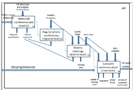
Figure 1.2 presents a representation of the communication system, from the statewide level down to the level of individual striping crews, used to manage striping operations (MoDOT 2015b):
On a statewide level, regional coordinators and/or district supervisors conduct weekly, statewide conference calls to discuss operations related to striping, plans and progress
On a regional level, regular phone conferences between the district supervisors in each region are conducted for discussion of weekly progress
At a crew level, constant communication using MoDOT radios between the driver of the striper and the operators regarding the quality of stripe is essential. Communicating via radio with the drivers on the crash truck and nurse truck is also important.
Figure 1.2 – Striping communications system
Crew leaders and operators are expected to perform two quality checks per day and add
information to the Missouri Accountability and Performance System (MAPS). The crew leader should record daily progress of lines striped per day and give this information to a district supervisor, who is expected to add this data to a database in order to keep track of the progress and next steps.
The length of a typical scheduled work day is 10 hours; this includes safety meetings, drive time to overnight locations, striping, and reloading time. Weather plays a key role in enabling or limiting striping operations; if a day begins with an expectation of cold weather (less than 35˚F) or rain, striping operations will not typically be performed. This is because the paint and beads may not properly adhere to the road surface if the temperature is low or conditions are too wet.
Striping equipment involved in pavement marking operation includes:
Striper (see Figure 1.3)
Middle warning truck
Shoulder advanced warning truck
The nurse truck (transports paint from bulk storage facility to location of striping operations)
Figure attribution: http://epg.modot.org/index.php?title=Image:620.2.jpg
Figure 1.3 – Striper
Although striping speeds vary based on factors such as elevation change, for the purpose of this analysis, we will assume that a crew stripes a non-divided highway at a speed of 10 miles per hour, and a crew stripes a divided highway at a speed of 8 miles per hour. The speed when not actively striping (deadheading) is assumed to be 35 miles per hour. When striping, the striper can paint two lines concurrently (as in Figure 1.3, in which the white edge line and double yellow center line are being striped at the same time).
Due to the slow moving nature of striping equipment, striping operations for even a small area (such as a county) take multiple days. As such, it would be inconvenient (and generate excessive deadhead miles) to return the striping vehicles to the assigned bulk storage facility at the end of each day. Instead, a striping crew’s vehicles (with the exception of the nurse truck) are parked overnight at the nearest MoDOT maintenance building (there are 25 such facilities in the Central District). The crew members return to the bulk storage facility at the end of the day in either a crew cab pickup or the nurse truck, these vehicles return the crew to their equipment at the start of the following day.
1.6 Striping Plan
Figure 1.4 – Old striping plan
According to the old plan, striping crews were expected to stripe 90% of the major roads before Memorial Day. After Memorial Day, they striped Regionally Significant roads and ramps. Then, with the remaining striping season, crews striped minor roads with cold weather paint, with a goal of striping 50% of minor roads each year (MoDOT 2015b).
Starting in 2015, striping policy changed. A new type of beads were introduced for divided highways; these beads required a high temperature for drying. Due to the difficulty of switching the type of beads in the striper, divided highways are now striped in one continuous time period. The new striping plan is represented in Figure 1.5.
In the early part of the striping season, when the weather is still cold (before June 1,
approximately), crews stripe minor roads. After this date, when the warmer weather is more conducive to striping divided highways with the new bead type (L), all divided highways will be striped. It is expected that striping on all divided highways will be completed by the end of July. From end of July until end of summer (while the weather remains warm), major undivided highways will be striped (with PM beads). As weather get colder, the rest of regional significant and minor roads will be striped until the end of the striping season (typically, mid-November) (MoDOT 2015b).
2. LITERATURE REVIEW
2.1 Road Striping Operations
We are aware of no optimization models that have been used for scheduling road striping operations. Most of the research papers examining pavement marking can be divided into the following categories:
Safety effectiveness of pavement markings. In (Smadi et. al.2008), the authors estimated how striping retroreflectivity levels might influence drivers, namely, whether it increases the safety of driving or makes it worse, due to drivers increasing their speeds.
Inventory and replacement of striping paint. In (Kouskoulas 1988), an inventory and replacement cost optimization model is presented for pavement marking system. Another study (Onyango et. al.2014) developed a degradation model of retroreflectivity that was represented as a function of time, environmental condition, and the number of traffic repetition after its application. Based on it, a degradation model was developed.
Pavement marking materials. An evaluation of various pavement marking materials used for longitudinal delineation was presented in (Taek et. al.1999), with the most cost-effective materials chosen based on the level of retroreflectivity and nighttime accidents. The influence of beads on retroreflectivity was examined in (Zhang et. al.2010).
2.2 Network Optimization Models
In the field of operations research, the Traveling Salesman Problem (TSP) is perhaps the best-known network optimization problem. The TSP’s objective is to determine the shortest route passing at least once through each of the nodes in a network; this route is further required to be a circuit, that is, the starting and ending node must be identical (Pieterse and Black 2014a, Laporte 2010, and Hoffman et. al.2001). A related problem, known as the Chinese Postman Problem (CPP), involves determining the minimum length route necessary to travel each arc of a network at least once (Guan 1962, Pieterse and Black 2014b, and Eiselt et. al.1995b). The Rural Postman Problem (RPP) is a slight variant to the CPP, in which the objective is to identify the minimum-length route that traverses a subset of the arcs in a network at least once (Eiselt et. al.1995a and Monroy-Licht et. al.2013). For MoDOT’s striping operations, because only a subset of all MoDOT road segments must undergo striping operations in a given year; the RPP provides a useful starting point for modeling.
vehicle, etc. These papers have considered both heuristic (evolutionary algorithm) (Weise et. al.2010) and exact (Cornillier et. al.2012) that could solve different kinds of VRP.
A final similar problem statement was presented in (Orloff 1974) and named the general routing problem (GRP). The GRP determines the minimum cost tour on a network, which starts and ends at the same node, and includes certain prespecified links and nodes in the tour.
2.2.1 Rural Postman Problem
As discussed above, the RPP shares many similarities with the problem of determining a minimum-length striping schedule. Many variations to the classic RPP model have been developed for particular applications.
RPP with turn penalties was introduced in (Benavent and Soler 1999). In this formulation, routes have to be operated on a street network, where some turns are forbidden and other turns are allowed but with some penalties.
Windy RPP, in which the cost of traversing an arc in one direction may be different from the cost of traversing it in the opposite direction, is examined in (Corberán et. al.2005a, 2005b, 2012 and Benavent et al. 2009).
RPP with time constraints (Monroy-Licht et. al.2013 and Letchford and Eglese 1997) considers situations in which the customers (arcs to be traveled) require service to occur within specific time windows.
Time-sensitive RPP (Tan et. al.2012), in which the travel (or service) time of each arc depends on the time interval during which the arc is traversed.
Mixed RPP (Corberán et. al.2005a, 2005b, 2012), in which the network has both arcs that must be traversed and specific nodes that must be visited.
While many applications of the RPP have been discussed in the literature (Eiselt et. al.1995a), no published study has examined the application of the RPP to scheduling striping operations. The RPP framework has been successfully applied to other roadway maintenance activities, such as winter gritting and snow removal operations (Li and Eglese 1996 and Jang et. al.2010). Striping operations and winter maintenance operations share similarities, as both consider road segments that may not require service, both attempt to minimize the total distance traveled by their
respective vehicles, and both involve vehicles that begin and end service at a “maintenance building” location. Similarly, multiple maintenance buildings exist within the winter
maintenance system, which roughly parallels the multiple maintenance building locations within the striping operation system.
In addition to winter maintenance, other applications of the RPP have explored fields such as delivery vehicle routing (Solomon 1987) and monitoring of roads for black-ice detection (Monroy-Licht et. al.2013). A shared aspect between these various applications of the RPP to vehicle routing problems involves the constraint of deadlines and time windows. In the case of winter maintenance operations, roads differ on classification, which result in variation in
deadlines and the time frames available to service various roads (Li and Eglese 1996). For black-ice detection, routing is largely dependent on information received from weather forecasts that determine intervals in which various road segments are available for monitoring (Monroy-Licht et. al.2013). Other instances of vehicle routing such as delivery and school bus routing generally impose time constraints due to customer priority and input regarding acceptable time windows (Solomon 1987).
Another factor differentiating the RPP as applied to striping operations from other applications is the requirement to pass some road segments more than one time. For the cases of garbage
collection and mail delivery, as discussed in (Eiselt et. al.1995a), an arc can generally be
considered to be “satisfied” with a single pass in either direction, whereas a multi-lane road may require two or more passes in order to completely mark all of the necessary lines. Additionally, the operations required to mark road segments is limited by a constraint requiring operations to move with traffic. For example, for an undivided road segment requiring stripes on the center line and on both edge lines, the first pass could travel from some Node X to Node Y, but, as a result, the second pass would have to travel from Node Y to Node X. One case of an RPP formulation with constraints on the direction of travel over arcs was used with a container
storage and retrieval facility in which the directed arcs corresponded to the storage or retrieval of containers across arcs (Vis and Roodbergen 2009).
However, no literature has been found addressing the unique combination of factors present in the system of striping operations such as directed arcs, multiple passes, and particularly slow-moving characteristics. In particular, the slow-slow-moving characteristics that make striping a continuous operation occurring over multiple months requires striping vehicles to overnight at a maintenance building at the end of each workday. This “overnighting” constraint requires a novel modeling approach to striping operations optimization. Accordingly, we will refer to our model as the slow-moving multi-pass postman problem with overnighting.
2.3 Genetic Algorithm
While the RPP is easily formulated, its solution is difficult (do Rosário Moreira and Ferreira 2010). Thus, most practical solution techniques make use of heuristic procedures such as Genetic algorithms (GA). As discussed above, our application involves a model that is even more
complicated than the classic RPP, thus an approach such as GA is needed to solve our problem..
minimum distance for a given sequence in this transformed network. The improvement for the order of nodes in the transformed network is achieved by Two-Opt and Three-Opt algorithms. These algorithms enable the authors to reduce computational complexity of calculating the shortest path distance for future generated orders due to nice applicability of the algorithms to the undirected network. Here, the shortest path algorithm applied to the new generated network gives which nodes (again each node represents a directed arc in the original undirected graph) are traversed in the shortest path, and thereby it eliminates the burden of determining direction of each traverse.
Another closely related study to ours that implements GA to the transformed graph is (do Rosário Moreira and Ferreira 2010). Here, the transformation process is achieved with a
somewhat similar method to that employed in (Groves and van Vuuren 2005). Each required arc is represented as a node without a direction and the distances between the nodes in the new generated graph are calculated by shortest path algorithm, the new problem then becomes a TSP. Since the graph is undirected, the authors in this study try to sequentially deal with optimizing both sequence and direction of all required arc traverses.
We chose to utilize a GA approach for our solution procedure. GA imitates an evaluation process so as to solve optimization problems, and it was initially proposed in (Holland 1975). This imitation process starts with generating an initial population, which is a set of initial individuals represented by chromosomes. Each generated chromosome has a value attribute known as fitness. Based on fitness score, the best ones are chosen in order to produce better chromosomes for future generations. Here, the selected chromosomes for GA are called parents, and
chromosomes produced from parents are known as children. The producing process is done by some operators of GA such as crossover, mutation and immigration. At each subsequent iteration, we implement these GA operators to the newly existing population, and we expect to generate a fitter population. The iteration of GA algorithm is continued in this reproducing process until a stopping criteria (e.g. maximum computational time) is met.
Having good GA operators significantly improves the performance of the algorithm. A well-designed GA should sustain the diversity of a population for the next generation. At the same time, it should also have some local optima search operators to reach improved solution in a reasonable period of time. The exact specifications of a particular problem make the definition of operators a problem-specific issue, thus a single best set of operators cannot be identified in advance for every problem.
In addition to having good type GA operators and parameters (e.g. crossover type and rate) in the iterations of GA, the performance of GA also depends on the quality of the initial population. Here, the quality strongly relates to not only average fitness of chromosomes but also diversity of the chromosomes in the population (Ahuja et. al.2000). Not having one of these properties leads to a less efficient GA. The underlying reasons of this conjecture are that fitter parents generally produce fitter children and that diversity enables us to avoid getting stuck at a local optima. Hence, determining a strategy for generating initial population and effectively implementing this strategy are crucial. In this regard, a Randomized Greedy Heuristic Method is implemented to generate the initial population for our analysis taking into account special network properties.
A further property that differentiates our problem from previous studies is that the different road types require a different striping strategy, and this causes the use of a different methodology to transform and represent the network (see discussion of “difficult segments” in Chapter 3). As an example, some roads require directed multi-passes (e.g. 2 directed traverses in one direction, 3 in the other), other roads can be traversed in any direction.
3. DATA ANALYSIS
3.1 Preparation of ArcGIS data
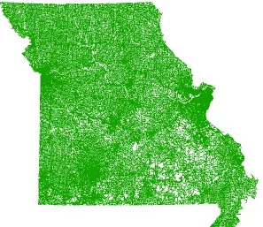
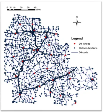
[image:28.612.160.457.209.466.2]ArcGIS files, such as ss_pavement_current, were provided by MoDOT. It includes the whole Missouri road network with MoDOT and non-MoDOT roads (Figure 3.1). The attribute table of this file includes all necessary information about road segments and has records about both directions of road arc (N and S, E and W).
Figure 3.1 – Missouri road network
highway. However, the geodatabase feature class file also included additional fields not included in either the Access or Excel file such as the number of lanes and whether a road segment
contains divided or undivided lanes. Another difference also includes the means by which road segments are defined. While the former files describe road segments as portions of roads between intersections of MoDOT maintained roads, the geodatabase feature class file describes road segments as portions of roads between intersections of other roads regardless of whether the intersecting road is maintained by MoDOT or not. As a result, a length of road between two intersections of MoDOT maintained roads may be described as a single road segment in the Access and Excel files, but, in the geodatabase feature class file, the road length may be described by multiple road segments due to the various road intersections not present in the former files. The division of road segments in the geodatabase feature class file may vary significantly in size from very small to representative of the entire road segment.
Due to the conditions in which MoDOT striping crews operate, the consolidation of the Access, Excel, and geodatabase feature class files was an important aspect of our preliminary analysis. To consolidate the data files, the first step involved creating a geodatabase feature class from the current MoDOT geodatabase feature class to reduce the contained set of cataloged road segments to only the segments maintained by MoDOT. In general, MoDOT is responsible for most
national and state highways across the state of Missouri. Some of the arcs eliminated from the new data set included city and county roads, which are maintained by either local government groups or contracted to outside agencies. In addition, the striping crews examined in our analysis only operated within the Central District, which permitted the further reduction of the data set to arcs contained within the 18 counties comprising the Central District of Missouri.
For this project we consider Central District roads, and only allow for travel to occur on MoDOT roads (with the exception of some nonMoDOT roads that are included to maintain connectivity of the network). We next have to make some modifications to prepare the data for use in our optimization model.
3.1.1 Creating the Junctions
The optimization model requires information about each arc: where it starts and where it ends, and how they are connected to each other. Starting and ending nodes have to be created for each arc. Creating the junctions in ArcGIS is a solution for that. The python code was developed to add junctions in the network. Necessary steps:
1. Creating Feature layers
2. Creating junction nodes – forming the end point for each line (only unique points should be kept)
3. Recording all the end points as JNode ID (making the feature layer for junction nodes) 4. Generating TO and FROM nodes fields in the main file.
5. A starting point of each line is the end point of previous line. An end point of a line is a starting point of next line (connected one)
8. Joining TNode (TO node) to End node and calculating values
9. Adding DEGREE field to Junctions layers (calculating the frequency of the node – how many lines has the same start or end point)
After running the code, the files Junctions (nodes) and District4 (segments) are created. The file with all lines includes around 20,000 segments. That’s a big size problem and there is a way to decrease the number of segments.
As it was mentioned previously, there are two records about the same segment: in E and W directions, in S or N directions. A divided road network was built based on projection in reality: S and N, E and W segments are a few meters apart from each other, then both records will be kept in the final data file. Concerning undivided roads, only one record is needed for the model (whether N or S, E or W). Keeping only one record will decrease data size, but aggregating of the arcs is needed as well.
3.1.2 Aggregation of the Arcs
Criteria for merging an arc:
Degree of the node =2
# of lanes is the same for both directions
If county name is the same
If designation and travelway name are the same
Road class is the same
As it was discussed above, there are three road classes: major, regionally significant, and minor. There is a field in attribute table of the main file MAJOR_MINOR. If it’s equal to Major, it means the class of the road is Major. If it’s equal to Minor, then the field
TW_CNTL_STATE_NAME should be considered. If this field includes CONTINUOUS OPERATION RT, then the segment is Regionally Significant. If the field is blank, then the road class of this segment is Minor.
For aggregation of the arcs another python code was created. Necessary steps:
1. Selecting arcs that intersect with junction of degree 2
2. Selecting fields for merging based on criteria discussed above.
3. Calculating the new length of merged arc, new FTnode information, keeping the minimum and maximum mile markers of segments merged (it will be kept in fields
BEG_CONTINUIOS_LOG and END_CONTINUOUS_LOG) 4. Keeping only one record for one direction (whether N or S, E or W)
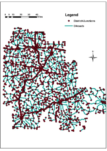
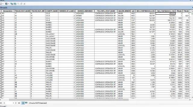
After running the code, D4Roads (all segments) and D4Junctions (nodes) files will be created (ArcGIS shape files). These files will be used as our Data. 6078 segments and 4881 nodes were created. The network with nodes and arcs is represented on Figure 3.2. (Central District MoDOT roads). The attribute table of file D4Roads is represented in Figure 3.3 (only necessary fields for the model are kept).
All divided roads are ready to be placed in an Excel file (the final input file for the model). As two records were kept for divided roads, difficult segments were not created. Undivided roads require additional analysis, as discussed below, for “difficult” segments.
3.2 Difficult Segments
As it was discussed above, “difficult” segments can be identified based on uid. The following steps should be performed:
1. Choose one county (e.g., Boone); choose only undivided roads of this county. (Choosing in ArcGIS can be performed with the tool Select by Attribute, and then exporting the data as a new layer).
2. Copy the data from attribute table (i.e., BooneUndivided) to excel 3. Sort the data based on uid from smallest to largest value
4. All uids with same value should be marked with a blue color (As a note, these segments couldn’t be merged, and records about both directions were kept for the same segment) 5. In step 4 above, groups based on the same uid were created. For each group find what was
the reason of not merging (whether number of lanes for each direction wasn’t the same, road class etc.)
6. Retain only one direction for segments (assumption: preferably save N and E if there are no other hard cases)
7. Make sure the connectivity of the network is maintained (when deleting the arc, from and to nodes are deleted as well. Don’t delete the nodes that connect “difficult” segments with others).
8. Calculate number of passes that are required for finishing the striping operation. 9. Choose Next County and repeat the algorithm from step 1. Stop when all counties are
completed.
Examples of “difficult” segments that might occur:
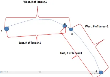
When end (or start) point of a segment in direction W is different from end (or start) point of segment in direction E (for undivided highways). The same case happens for S and N
direction segments as well. The example is represented in Figure 3.4. There are segments from node 1 to node 4 of road RT M that has the same uid. In ArcGIS there is a record about segment 1-3 in W direction, # of lanes =1, segment 3-4 in W direction, # of lanes =1. Also, there is record about segment 1-2 in E direction, # of lanes=1, segment 2-4 in E direction, # of lanes=1. Number of lanes is the same for both direction, but because they act differently in both directions the code couldn’t merge these arcs and kept the record about both cases in the attribute table. (end and start points are different).
Solution: two segments with only one direction should be chosen (E in this case). The records about two other segments (W in this case) will be deleted.
Figure 3.4 – Example of “difficult segment” (end and start points are different)
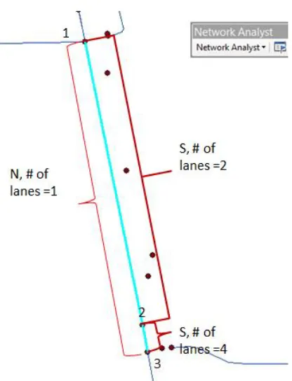
When segments have different number of lanes in both directions. Example is represented in Figure 3.5. The code couldn’t merge the segments from node 1 to node 3 and kept records about both direction (N and S). As we can see segment in N direction has only 1 lane but it’s changing in S direction from 2 lanes to 4 lanes. It happens in cases when other roads intersect with this road. Road segment MO 163 from 1-to 3 has a record in N direction and # of lanes =1. Road segment MO 163 from node (1-to 2) = S direction, # of lanes =2. Road segment MO 163 (2-3) = S direction, # of lanes =4.
Solution: In order to decide how to treat this kind of segments we have to know how many passes should be made for each segment in order to finish the striping operation (calculating number of passes will be discussed in Section 3.3). Segment 1-2 will require 2 passes (if striping starts from one-lane side N (edge line and center line)). Segment 2-3 will require 3 passes (if striping starts from one-lane side N). It’s better to keep records about the two segments in S direction because these two segments will be striped differently, and delete the record about the segment in N direction.
Figure 3.5 – Example of “difficult” segment (# of lanes is not the same)
When segments have different number of lanes and passes, and different end or start points in both directions. The example is represented in Figure 3.6. This is a combination of the first and second type of “difficult” segment when the behavior of segments is totally different in both directions.
The segment from node 1 to node 6 couldn’t be merged because in N and S they have a different number of passes, and also, start and end points are not the same. Analysis of the number of passes required has to be made for each segment in each direction.
Let’s choose to save N segments. If striping of double yellow line and white edge line (or white center line) is started from N direction than the number of passes for segment 1-2 will be equal to 3 (S side is one-lane road). With the same, the logic number of passes for segment 2-5 is equal to 2 (for one-lane, two-lane and then one lane segment again). The number of passes for segment 5-6 is equal to 3 (S side is one-lane road)
Let’s choose to save S segments. The assumption about starting striping from N is kept. It’s hard to calculate number of passes for segment 1-3 because for part of segment 1-2 it’s required to have 3 passes but for part of segment 2-3 only 2 passes. Number of passes for segment 3-4 = 2. It’s hard to calculate number of passes for segment 4-6 as well because in area of segment 4-5 it’s required to have 2 passes but for segment 5-6 is 3. It seems it’s not preferable to save records for S segments because for some parts of the segments the number of passes won’t be the same. It’s better to choose the segments in direction where the full segment can be striped with the same number of passes.
Figure 3.6 – Example of “difficult” segment (# of passes and end/start points are different)
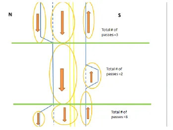
How this assumption (in what direction to start striping the first 2 lanes (usually double yellow line and edge line (white center line))) works in reality is represented in Figure 3.7. We assumed that striping would be started from N, and the record about segments in N direction only will be saved. Now it is easy to calculate the required number of passes.
.
[image:36.612.140.489.422.684.2]There are longer and harder segments in the network that the code could not merge for similar cases. These were treated the same way as the three previous types. For most of the cases an assumption about the starting direction was made. In the Excel file, the column with information about the opposite direction is added (how many lanes the opposite direction has).
When segments are disconnected from the network. It means there are no MoDOT roads in Central district that can connect them with others. These kind of roads are marked with “pink” color in the Excel file. The example is shown in Figure 3.8.
[image:37.612.137.476.244.451.2] Solution: Non-MoDOT roads or roads from other districts can be added to the network. That disconnected segment can be reached by passing these roads. Added roads were marked with a green color, and they don’t require striping.
Figure 3.8 – Example of disconnected segment
3.3 Calculation of Number of Passes
It’s very important to know how many times each segment should be passed for finishing the striping process for optimization model. The strong logic has to be developed.
3.3.1 Calculation Logic for Number of Passes for Divided Roads
Table 3.1 – Calculation of number of passes for divided roads # of lanes for one side
(N, S, E, W) # of passes
Scheme for how passes will be made
1 lane 1 pass
2 lanes 2 passes
3 lanes 2 passes
4 lanes 3 passes
3.3.2 Calculation Logic for Number of Passes for Undivided Roads
We only consider segments for this Section that have the same number of lanes for each side. The calculation logic for number of passes for undivided roads is described in Table 3.2.
Table 3.2 – Calculation number of passes for undivided roads
# of lanes for N or E side
# of lanes for S or W side (opposite direction)
# of passes
Scheme for how passes will be made
1 1 1 If only center line should be striped
(no edge lines)
1 1 2
OR
2 2 3
3 3 4
In this case an assumption about the starting direction (where striping starts) is not required. No matter where the start is, the number of passes will be the same.
The striper can paint two lines at the same time. Based on discussions with MoDOT, the decision was made that it is more preferable to stripe two lines of different color in terms of usage of paint. If there is a choice it is better to stripe yellow center line and white edge line (or white center line) together.
In Table 3.2, the case of two-lane road is represented when number of passes required for striping is equal to one. Usually, this kind of road only has the center line. There are no edges that require striping. In order to identify these segments, the Excel file Striping progress should be checked. If in column White E/L, there are no numbers (length information), it means that no white paint should be used for the edges (Figure 3.9). Only the yellow center line will be painted. Then, only one pass is required to finish this center line. These segments are marked with orange in the Excel file (final data).
Table 3.3 – Calculation of number of passes for “difficult” segments # of lanes for N or E side* # of lanes for
S or W side (opposite direction)
# of passes
Scheme for how passes
will be made Notes
0
2
2 The same logic as for
divided roads because road can be passed only in direction
0 3 2 //-//-//
1 2 2 Assumption: Striping will
be started from one-lane side
2 1 3 Assumption: Striping will
be started from two-lane side
1 3 3 No matter where striping
will be started, number of passes will be the same
1 4 3 Assumption: Striping will
# of lanes for N or E side* # of lanes for
S or W side (opposite direction)
# of passes
Scheme for how passes
will be made Notes
2 3 4 Assumption: Striping will
be started from two-lane side
3 2 3 Assumption: Striping will
be started from three-lane side
2 4 4 No matter where striping
will be started, number of passes will be the same
2 5 4 Assumption: Striping will
# of lanes for N or E side* # of lanes for
S or W side (opposite direction)
# of passes
Scheme for how passes
will be made Notes
3 4 4 Assumption: Striping will
be always started from three-lane side in order to have the minimum number of passes
3 5 5 No matter where striping
will be started, number of passes will be the same
3 6 5 Assumption: Striping will
be always started from three-lane side in order to have the minimum number of passes
5 4 5 Assumption: Striping will
be always started from five-lane side in order to have the minimum number of passes
* Assumption: Start striping double yellow line and white edge line (centerline) from this direction
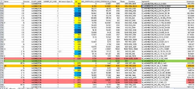
3.4 Final Excel Data File: MoDOT Roads
3.3.3 Calculation Logic for Number of Passes for “Difficult Segments” (Undivided Roads)
All the different cases of “difficult” segments that were met in the network are represented in Table 3.3. For “difficult” segments it’s important to know how many lanes the opposite side has. This is going to influence the final number of passes required for striping. A key assumption needs to be made regarding from which side (E or W, N or S) striping operations should be started. In Table 3.3 the starting side (direction) will be in column 1. The second column
includes information about opposite side. In most cases, the starting direction will be the one that gives the minimum number of passes. Column Notes details what assumption was used here. Also, there is a scheme how striping passes should be made in reality.
As a summary:
Blue /dark blue color identifies “difficult” segments
Orange color identifies two-lane undivided roads with center line only (1 pass)
Pink color means that segment was disconnected from the road network
Green color shows added roads (nonMoDOT roads or roads from other districts)
Yellow color just marks all uids. Important fields that will be used in the model: Designation, Name, Direction, County name, Number of lanes, Number of lanes of opposite side, uid,
Beg_Continuous_Log, End_Continuous_Log (mile marker), FNode, TNode, Distance in meters and miles, Class of the road, Divided_Undivided class, number of passes, NeedStripe(0,1). NeedStripe(0,1) field defines whether the segment should be striped this year (1) or not (0). This decision has to be made by MoDOT district supervisor. SegmentID field will be the main output from the model: Direction_County_Designation_Name_MileMarker(Beg_End).
3.5 Overnight Location Distances File
Note: subsequent to the creation of this map, we were informed that the maintenance facility at Hallsville was recently closed; this Hallsville facility has been removed from our models.
Figure 3.11 – Map with overnight locations
The striping crew finishes their job at some node (end of a segment) at the end of each day. For this node they should choose the closest overnight location. It’s necessary to know the closest facility for each node and distance to it for the model. There is a Network Analysis tool in AcrGIS that can help to calculate all the distances from each node to its closest facility. The following steps shall be made:
1. Make sure that catalog is visible in ArcGIS. There is a folder that includes all our shape files described above (District4Roads.gdb). Find it in catalog-> right click on this folder ->choose New->Feature Dataset. Create a new feature dataset and give it the name (i.e., try).
3. In processing window choose the input – the network that will be used for finding the best route. If we choose only MoDOT roads distances won’t be calculated for all nodes because some segments are disconnected. The network with all MoDOT roads was used
(ss_pavement_current). The file all roads will be created (Figure 3.12).
Figure 3.12 – Creating the feature class in ArcGIS
4. Then after necessary data is added, the network dataset should be created. Right click on created folder try -> New -> choose Network Dataset. The files try_ND and
try_ND_Junctions will be created. The file with junctions will be the same as District4_Junctions.
5. Make sure that Network Analysis tool is enabled. (Customize->Toolbars). Then go to network analysis panel -> choose the network dataset try_ND. In network analysis catalog choose New Closest facility.
Figure 3.13 – Loading facilities step
7. Incidents correspond to the nodes. Right click -> Load locations -> choose file D4_Junctions. 8. If all facilities could be allocated they would be represented with a big red circle. If all
Figure 3.14 – Allocation of facilities and incidents
Figure 3.15 – Solution of closest facility tool
Figure 3.16 – Attribute table of Routes
10.1. Right Click on Routes -> Joins and Relates -> Join. In the processing window choose the field in Routes that the Join will be based on – ObjectID. Load table
District4_Junctions (there is information in this file about JNodeID and ObjectID). Choose the field in Added Table – ObjectID. All the fields from District4_Junctions will be joined to Routes file. We just need to keep JNodeID.
10.2. In order to make other modifications it’s better to create another file identical to routes. Right click on Routes->Export Data-> Give the name OvlD.
10.3. In order to add the field with county names, it’s necessary to have a unique name for each facility. In OvlD file add a new field OVLName. Right click on this field-> Field Calculator-> type = (!Name!).replace(Location, “ “). Then replace all numbers with this name.
10.4. For removing all extra spaces before Name add new field OName -> Right click on it -> Field calculator -> type =LTrim([OVLName]). This code will remove all spaces and name will be in the required format.
11.After all these steps with modifications are done, the data is ready to be placed in excel file (Figure 3.17). It includes nodes ID (JnodeID), closest overnight location name, facility county name, FacilityID, Distances in miles and meters, and the node from the network that is closest to each facility.
[image:52.612.75.540.142.351.2]
4. GENETIC ALGORITHM MODEL
In this chapter, the following are presented: a) brief description of our GA, b) installation process of required programs and libraries for our program, and finally c) usage of our program interface.
4.1 Brief Description of the GA
We do not directly apply a GA to the RPPs. Therefore, as a first step, we converted RPP to equivalent TSP. Here, each required arc to be striped in RPP is represented as a node in TSP. The shortest distances among all nodes in TSP are calculated by Dijkstra’s Algorithm.
Meanwhile, when we make such conversions, we take the road segment’s properties into account such as type of the road (divided/undivided), number of traverses, etc. After completing data preparation, we implemented Randomized Greedy Heuristics to get a better initial solution and thereby to improve the final solution produced by GA. In addition to this, improving GA’s performance is strongly related to using appropriate GA operators as mentioned earlier. In this regard, we implement the exchange, insertion and direction mutations and binary crossover operations. Here, we do not take overnighting into account during application of those operators. However, later, overnighting locations are inserted to the striping sequence. By doing so, we take the advantage of similarities between solution sequences and thereby we decrease the
computational time. The GA’s operators we used are:
Binary Crossover: In binary crossover, we randomly choose 2 individuals (Individual 1 & Individual 2) from the population to produce a child as shown in Figure 4.1.
Figure 4.1 – Binary crossover
Here, we have 8 required arcs in the original graph and each of them is represented as a node as shown in the table. Later, we randomly generate a binary vector. In this binary vector, whenever we see 1, we copy the corresponding node from individual 1 to the child. We make a list of nodes corresponding to 0 in the binary vector and we check how those nodes are ordered in Individual 2. Finally, we place the remaining nodes corresponding to 0 in the binary vector as seen in the order of Individual 2. The last column shows the fitness values of individuals and child.
Insertion Mutation (IM): We apply IM to the child generated from binary crossover to produce a fitter individual and then we replace the worst individual in the population by this new
individual. Here, we examine some possible insertion positions and select the best positions among those considered in terms of fitness value. The computational expense here is low.
Figure 4.2 – Insertion mutation
Exchange mutation (EM): We again randomly select an individual (I3) from the population to produce a child (C3), replace I3 by C3. We do a somewhat similar approach in Insertion
mutation.
Figure 4.3 – Exchange mutation
Direction mutation (DM): Once the final population is determined, we optimize the direction for each arc requiring an odd number of passes for each individual.
As a next step, we integrate the overnighting piece of our problem to our GA to calculate the actual fitness of each individual generated by GA’s operators. Here, daily working hours, deadheading speed, striping speed are some of the important parameters that affect the end node of each striping day and thereby the overnight location of that day.
With the components of GA we have mentioned, we are able to provide an efficient striping schedule to reduce deadhead miles. It does not require manual intensive work except for entering some input parameters, and it enables the users to do some what-if analysis to examine the impact of resource levels such as daily working hours.
4.2 Installation Process of Required Programs and Libraries
[image:55.612.85.528.305.670.2]The installation process is shown sequentially. These installation directions assume that the Python program has not already been installed on the computer. First, install Python 2.7.2 from the website: https://www.python.org/download/releases/2.7.2/ using setup’s default setting.