Refilling process in the plasmasphere: a 3-D statistical characterization based on Cluster density observations

Ann. Geophys., 31, 217–237, 2013 www.ann-geophys.net/31/217/2013/ doi:10.5194/angeo-31-217-2013

© Author(s) 2013. CC Attribution 3.0 License.

EGU Journal Logos (RGB)

Advances in

Geosciences

Open Access

Natural Hazards

and Earth System

Sciences

Open Access

Annales

Geophysicae

Open Access

Nonlinear Processes

in Geophysics

Open Access

Atmospheric

Chemistry

and Physics

Open Access

Atmospheric

Chemistry

and Physics

Open Access

Discussions

Atmospheric

Measurement

Techniques

Open Access

Atmospheric

Measurement

Techniques

Open Access

Discussions

Biogeosciences

Open Access Open Access

Biogeosciences

Discussions

Climate

of the Past

Open Access Open Access

Climate

of the Past

Discussions

Earth System

Dynamics

Open Access Open Access

Earth System

Dynamics

Discussions

Geoscientific

Instrumentation

Methods and

Data Systems

Open Access

_{Geoscientific}

Instrumentation

Methods and

Data Systems

Open Access

Discussions

Geoscientific

Model Development

Open Access Open Access

Geoscientific

Model Development

Hydrology and

Earth System

Sciences

Open Access

Hydrology and

Earth System

Sciences

Open Access

Discussions

Ocean Science

Open Access Open Access

Ocean Science

Solid Earth

Open Access Open Access

Solid Earth

Open Access Open Access

The Cryosphere

Natural Hazards

and Earth System

Sciences

Open Access

Discussions

Refilling process in the plasmasphere: a 3-D statistical

characterization based on Cluster density observations

G. Lointier1, F. Darrouzet2, P. M. E. D´ecr´eau1, X. Valli`eres1, S. Kougbl´enou1, J. G. Trotignon1, and J.-L. Rauch1 1_{Laboratoire de Physique et Chimie de l’Environnement et de l’Espace, UMR 7328 CNRS/University of Orl´eans, 3A avenue} de la recherche Scientifique, 45071 Orl´eans cedex 2, France

2_{Belgian Institute for Space Aeronomy (IASB-BIRA), Brussels, Belgium}

Correspondence to: G. Lointier ([email protected])

Received: 30 June 2011 – Revised: 1 October 2012 – Accepted: 2 October 2012 – Published: 8 February 2013

Abstract. The Cluster mission offers an excellent opportu-nity to investigate the evolution of the plasma population in a large part of the inner magnetosphere, explored near its or-bit’s perigee, over a complete solar cycle. The WHISPER sounder, on board each satellite of the mission, is particu-larly suitable to study the electron density in this region, be-tween 0.2 and 80 cm−3. Compiling WHISPER observations during 1339 perigee passes distributed over more than three years of the Cluster mission, we present first results of a sta-tistical analysis dedicated to the study of the electron den-sity morphology and dynamics along and across magnetic field lines betweenL=2 andL=10. In this study, we ex-amine a specific topic: the refilling of the plasmasphere and trough regions during extended periods of quiet magnetic conditions. To do so, we survey the evolution of the ap in-dex during the days preceding each perigee crossing and sort out electron density profiles along the orbit according to three classes, namely after respectively less than 2 days, between 2 and 4 days, and more than 4 days of quiet magnetic condi-tions (ap≤15 nT) following an active episode (ap>15 nT). This leads to three independent data subsets. Comparisons between density distributions in the 3-D plasmasphere and trough regions at the three stages of quiet magnetosphere provide novel views about the distribution of matter inside the inner magnetosphere during several days of low activ-ity. Clear signatures of a refilling process inside an expended plasmasphere in formation are noted. A plasmapause-like boundary, atL∼6 for all MLT sectors, is formed after 3 to 4 days and expends somewhat further after that. In the outer part of the plasmasphere (L∼8), latitudinal profiles of me-dian density values vary essentially according to the MLT sector considered rather than according to the refilling

dura-tion. The shape of these density profiles indicates that mag-netic flux tubes are not fully replenished after 6 days of quiet conditions. In addition, the outer plasmasphere in the night and dawn sectors (22:00 to 10:00 MLT range) maintains an overall clear deficit of ionospheric population, when com-pared to the situation in the noon and dusk sectors (10:00 to 22:00 MLT range).

Keywords. Magnetospheric physics (Plasmasphere)

1 Introduction

The plasmasphere consists of a cold (≤1 eV) and dense (10– 104cm−3) torus of plasma that co-rotates with the Earth, forming the innermost region of the magnetosphere (Carpen-ter, 1963; Nishida, 1966; Lemaire and Gringauz, 1998). Its outer edge, the plasmapause, has been recently referred to as the Plasmasphere Boundary Layer, or PBL, because of the complexity and variability of the plasma population that can exist near this boundary and because of the variety of criteria used to define it (Carpenter and Lemaire, 2004). It is widely recognised that the plasmasphere is a very dynamic system highly constrained by both the solar wind and the ionosphere via the solar wind driven convection electric field, the electric field associated with the Earth’s rotation and the interchange fluxes between the ionosphere and magnetospheric regions at higher altitude. Variations of these large-scale processes and their interplay affect the configuration and the dynam-ics of the plasmasphere, i.e. have an impact on the plasma distribution in space and time and govern the PBL formation (Darrouzet et al., 2009a).

The arrival of a solar wind perturbation at Earth induces an increase of the convection electric field. The convecting flux tubes outside the co-rotation region drive their plasma content sunward toward the magnetopause (McFadden et al., 2008) before being ultimately driven tailward (Chandler and Moore, 2003; Elphic et al., 1997). During disturbed geomag-netic periods, the convection electric field is strong enough to erode outer regions of the plasmasphere. The most spectac-ular feature of the plasmasphere dynamics under a geomag-netic activity increase is the formation of drainage plumes (elongated structures of cold plasma) in the afternoon local time sector (Goldstein et al., 2004; Darrouzet et al., 2008). The density transition at the PBL gets sharper and moves earthward, belowL=3, on timescale of a few hours (Car-penter, 1967; Chappell et al., 1970; Carpenter and Anderson, 1992; Moldwin et al., 2002). Additional processes such as the subauroral ion drift and various wave activities can affect the spatial distribution of the density at the PBL (De Keyser et al., 1998; Moldwin et al., 1997).

The refilling process of the plasmasphere, continually sup-plied by escaping particles from the dayside ionosphere along the co-rotating flux tubes, is more effective during ex-tended periods of low geomagnetic activity (Kp<1+, i.e.

ap<5 nT) (Darrouzet et al., 2008). Two or three days of re-filling are typically required for plasma density to reach high values at geosynchronous orbit and beyond, but this time in-terval is not sufficient for diffusive equilibrium with the iono-sphere to be established (Moldwin et al., 1994; Spasojevi´c et al., 2003). In contrast, Reinisch et al. (2004) reported a sig-nificant filling in less than 28 h at lower altitudesR=2.5RE. The unexpected long refilling time of flux tubes in the outer plasmasphere implies that a transport mechanism, in addi-tion to co-rotaaddi-tion and convecaddi-tion, drifts the plasma outward across the geomagnetic field lines. The existence of a plas-maspheric wind mechanism was first predicted by Lemaire and Schunk (1992), and observed later by Dandouras (2008). The description of the plasmasphere’s dynamics assumes that the PBL is always observable due to the continuous interplay between the convection electric field and the co-rotation one. In that line of thought, several studies have been achieved to elaborate an empirical relationship between the PBL location and the geomagnetic indices (Carpenter and Anderson, 1992; Moldwin et al., 2002), and between the PBL location and the solar wind conditions (Larsen et al., 2007). However, observations of smooth plasmaspheric den-sity transition extended toL=7 and beyond have been re-ported after several days of quiet geomagnetic conditions (Chappell, 1972; Carpenter and Anderson, 1992; Tu et al., 2006). This implies either a PBL located beyondL=7 or a smooth density transition from the inner plasmasphere up to the sub-auroral region without detectable signature of a distinct boundary. Such a smooth transition is possible if the co-rotation dominates over the convection at large radial dis-tance. Tu et al. (2007) presented some cases of extended plas-masphere having smooth density transition for weak

geo-magnetic activity (Kp<3) during two or more days. They

suggest that this is indirect observational evidence of the plasmaspheric wind. Little attention has been paid to model such a smooth density transition at the PBL. Actually, ignor-ing the density distribution along depleted flux tubes is a real difficulty when one wishes to undertake and validate simula-tions of plasmasphere filling/refilling (Tu et al., 2004, 2006, 2007).

Wave and particle interactions impact the density distri-bution inside the plasmasphere (Liemohn et al., 1997). Con-versely, knowledge of the electron densitynein the plasma-sphere and its outer edge is necessary to study how dense cold plasma can affect whistler-mode waves that scatter radi-ation belt electrons (3< L <7). Many studies demonstrated that the presence of ElectroMagnetic Ion-Cyclotron (EMIC) waves (Summers and Thorne, 2003; Spasojevi´c et al., 2004; Borovsky and Steinberg, 2006; Usanova et al., 2010), plas-maspheric hiss (Lam et al., 2007) and whistler-mode cho-rus (Summers et al., 2004) at the PBL and within the drainage plumes can pitch-angle scatter relativistic electrons during storms (at different time scales, depending on the waves). Borovsky and Denton (2009) show clear evidence that buildup of the outer plasmasphere plays an important role in the decay of the radiation belt electrons (∼150 keV) during intervals of extreme geomagnetic calm. Ring current protons may also be lost due to EMIC waves (Spasojevi´c et al., 2004). It is necessary to model the density distribu-tion along the magnetic field lines in order to understand the growth of these waves and their impact on the plasma popu-lations.

Most thermal plasma density models are empirical. The model of Carpenter and Anderson (1992) describes the equa-torial electron density based on the near equaequa-torial ISEE-1 radio measurements. The IZMIRAN model by Chasovitin et al. (1998) and the Global Core Plasma Model (GCPM) by Gallagher et al. (2000) yield vertical profiles of plasma-spheric density as a function of solar and geomagnetic ac-tivities. Sheeley et al. (2001) used CRRES observations to describe the density inside and outside the plasmasphere. In these models, an electron density profile of Lα (with

trajectory crosses a particular field line at two different points (one in each hemisphere). Tu et al. (2006) extended the tech-nique used by Reinisch et al. (2001, 2004) and Huang et al. (2004) to model the field-aligned electron density profile re-motely from the Radio Plasma Imager (RPI) on board the IMAGE satellite. They concluded that the power law depen-dence quoted above is reliable enough to construct global empirical plasmasphere/trough models. They discussed the feasibility of determining the density profile along depleted flux tubes but they could not obtainne0 because measure-ments covered only one hemisphere at a time. These studies reveal all the inherent difficulty in reconstructing density pro-files along magnetic field line from direct in situ and remote data. Nevertheless, the density variations across the fields lines are more pronounced than those along the field lines (Darrouzet et al., 2006) and the parallel velocity of the elec-tron is almost constant among the field lines (Tu et al., 2005). This suggests that a statistical approach can be suitable to study field-aligned density distribution in the plasmasphere region.

Based on a statistical description of the WHISPER obser-vations taken on board the Cluster satellites, this paper fo-cuses on the latitudinal dependence of the electron density along the magnetic flux tubes and its evolution during ex-tended intervals of low magnetic activity. After a presenta-tion of the instrumentapresenta-tion and of the method used to elab-orate the database (Sect. 2), statistical results are discussed in Sect. 3. The last section summarises our findings and dis-cusses their perspectives.

2 Cluster plasmaspheric coverage

The ESA’s Cluster mission, launched in 2000, is a constel-lation of four identical spacecraft (referred to here as C1, C2, C3 and C4) flying in a tetrahedral configuration (Es-coubet et al., 1997). The Cluster mission has been designed to study the small-scale structures and macroscopic turbu-lence in three dimensions in many regions of the magneto-sphere (magnetopause, polar cusps, magnetotail and the au-roral zones) as well as the solar wind upstream of the bow shock (Escoubet et al., 2001). The four spacecraft have orig-inally evolved along a quasi-polar orbit, with a perigee at 4.2RE, an apogee at 19.6REand a periodicity of about 57 h. Cluster orbit precession covers a local time sector of about 0.15 h between two perigee passes, enabling spacecraft to cross the aforementioned regions at all local time sectors in one year. During the nominal part of the mission, the inter-spacecraft distance was changed several times, ranging from 100 km to 10 000 km. Since 2005, the constellation has been altered from a tetrahedral configuration to a multi-scale ge-ometry; C1, C2 and C3 kept the same separation distance while C4 orbited at closer distance to C3 (down to 17 km). The plasmasphere region, which is the region of interest for this study, was not one of the primary scientific objectives.

10 5 0 -5 -10

XSM[Re] -10

-5 0 5 10

ZSM

[

R

e

] 2003 Mar

2009 Mar

10 5 0 -5 -10

YSM[Re] -10

-5 0 5 10

ZSM

[

R

e

]

2009 Mar

2003 Mar

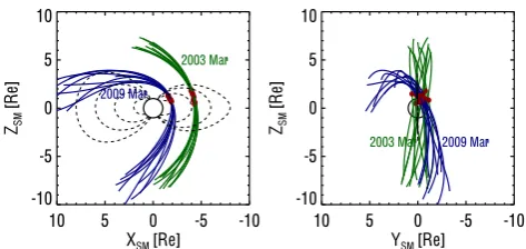
Fig. 1. Example of successive perigee passes by C2 for March 2003

(green) and March 2009 (blue) projected in SM coordinates. Dashed black lines draw magnetic field lines estimated by the geomagnetic model IGRF-11 + Tsy04. Red dots are placed at the perigees of the plotted orbits.

However, the high eccentricity of the Cluster’s orbit enables spacecraft to dive deeply enough into the inner magneto-sphere to cross the plasmaspheric region. During the first years of the mission, a large range of latitudes over a limited local time interval is explored at each perigee crossing. The PBL is typically located in the 3< L <8 range at the equa-tor, depending on the level of geomagnetic activity (Carpen-ter and Lemaire, 2004). Darrouzet et al. (2009a) reviewed the contribution of the Cluster mission in our understanding of the plasmaspheric structures and dynamics and also its con-tribution to recent advances in the description by models.

in 2010 (above 25◦_{N). The perigee, which explored regions} near apex of magnetic field lines in 2003, explored regions closer to their magnetic foot in 2010. It is important to note that from the middle of the year 2008, the Cluster orbit en-ters twice the plasmasphere. The spacecraft cross the inner plasmasphere from South to North in a given local time sec-tor, heading toward perigee, then fly over auroral regions and polar cap at higher altitudes. Finally, the spacecraft en-ter again in plasmaspheric magnetic flux tubes located at 6< L <9 in a local time sector opposite to that of the in-bound crossing, travelling from the Northern to the Southern Hemisphere at a slower velocity (during a longer time inter-val) than inbound. During the years selected for this analy-sis, the satellites generally leave the plasmasphere during the second crossing before reaching the equator. We discuss in Sect. 2.2 the specifics of electron density sampling during the second plasmasphere crossing. Independently of the num-ber of times the orbit enters and leaves the plasmasphere or trough regions near a given perigee, we define a density pro-file as constructed from all density records measured along that perigee pass by a given Cluster satellite.

Figure 1 illustrates that, in addition to a slow evolution over the years, the spacecraft cross the magnetic field lines at different locations from one orbit to another. This is a consequence of the Earth rotation coupled with the magnetic dipole tilt. Projected onto the X-Z and X-Y planes in SM co-ordinates, the position of the perigee (red dot) varies greatly in latitude and in local time. This variability is enhanced un-der the effect of geomagnetic activity variations and gives ac-cess to a larger range of latitudes along magnetic field lines.

2.1 Electron density determination

We use data obtained from one of the eleven Cluster instru-ments, called Wave of HIgh frequency and Sounder for Prob-ing Electron density by Relaxation (WHISPER) to estimate the electron density (D´ecr´eau et al., 1997). Particle instru-ments on board Cluster spacecraft cannot be used to estimate the electron density in this region. The PEACE instrument (Johnstone et al., 1997), measuring electrons in the low en-ergy range (10 eV–26.5 keV), is switched off most of the time near the perigee due to the presence of high energetic popu-lations in the inner magnetosphere (mainly in the radiation belts and lesser in the ring current population), which can be hazardous for particle measurements. WHISPER is a re-laxation sounder providing a diagnosis of the local particle populations from triggering resonances in the plasma in ac-tive (sounding) mode and from monitoring the natural elec-tric waves in passive mode (D´ecr´eau et al., 1997, 2001).

In this work, we present electron density estimates ob-tained after an analysis of frequency spectra obob-tained dur-ing both operation modes (sounddur-ing or passive). This analy-sis carries out a direct or indirect identification of the elec-tron plasma frequency Fpe, related to the electron density

neasFpe[kHz] ≈9

√

ne [cm−3]. The WHISPER instrument

10 20 30 40 50 60

dB above 10

-7 V

rms

.Hz

-1/2

2 20 40 60 80

Frequency (kHz)

C2

HBR NBR

overflow Method: Average

UT 07:00:00 08:00:00 09:00:00 10:00:00 11:00:00 12:00:00 13:00:00 14:00:00 15:00:00

R(Re) 7.66 6.30 4.88 3.57 3.07 3.91 5.28 6.70 8.02

Lat_sm(deg) -82.41 -82.44 -62.85 -27.00 32.46 84.05 61.45 42.39 29.02

LT_sm(h) 23.19 15.54 14.16 14.05 14.26 17.81 1.42 1.80 2.00

Fce FpeFUH 2FceFq2 3Fce Fq3

FUH

Fq2 2Fce

3Fce

Fq3

auroral hiss

Fce

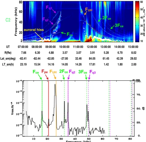
Fig. 2. Example of an asymmetric plasmasphere crossing, on 9

Au-gust 2007, 07:00–15:00 UT. Top panel shows the spectrogram recorded by C2. Bottom panel displays a spectrum recorded at 09:16:10 UT. Typical resonances observed in the plasmasphere are indicated on both panels by arrow of given colours: orange for

up-per hybrid frequency (FUH), green for gyro-harmonic (nFce) and

purple for Bernstein modes (Fqn). The plasma frequency Fpe

de-rived from the diagnostic is plotted as white dots in the top panel (it is an identified resonance pointed by a red arrow in the bottom panel). Auroral hiss emissions (top panel) are pointed by a yellow arrow.

can thus estimate electron densities for values up to 80 cm−3 with a temporal resolution of 2 s on average. The estimated spatial resolution of electron density observed is of the or-der of 1 km, i.e. a few times the electric antenna tip-to-tip lengthd, withd=88 m. The electron density determination has been carried out in two steps: (1) a semi-automatic tool dedicated to the density production for the Cluster Active Archive (Trotignon et al., 2010) has been first applied; (2) the obtained electron density profiles are then checked man-ually in order to correct or filter spurious points.

In the plasmasphere, resonances arise at the electron gyro-frequency Fce (and its harmonics nFce), the total electron plasma frequencyFpe, the upper-hybrid frequencyFUH and the Bernstein’s mode frequencies Fqn (Bernstein, 1958). Note that local wave cut-off properties can also be used to determineFpe (Canu et al., 2001). We can further mention the lower hybrid frequency,Flh, observed since 2009 at alti-tudes below∼4000 km (Kougbl´enou et al., 2011).

resonances allowing electron density to be accurately deter-mined (Trotignon et al., 1986, 2010). White dots point out theFpe profile along the orbit. For an active spectrum, the

Fpevalue is deduced semi-automatically from the diagnostic ofFUHandnFceseries, which are related together by the re-lationFUH=

q

Fpe2+Fce2.FUHis assumed to be the most intense resonance in a frequency band manually selected (Trotignon et al., 2010).Fce is derived from the magnetic field measurement provided by FGM (Balogh et al., 1997) (Fce [kHz] =28.10−3×B0[nT]). The high frequency limit of the instrument, 80 kHz, is also the highest observable value ofFUH. The highest plasma frequency measurable,Fpe max around perigee, is controlled by the gyrofrequency value, and is smaller than 80 kHz.Fpe maxis always close to 80 kHz dur-ing the first part of the mission when perigee is at 4RE and the gyrofrequency Fce below ∼20 kHz (Fpe max=77 kHz whenFce=20 kHz). Later in the mission phase, the gyrofre-quency at perigee increases with decreasing radial distances and increasing latitudes. For instance, the gyrofrequency value isFce∼40 kHz at a magnetic latitude of 50◦and a ra-dial distance of 3RE, which leads toFpe max=70 kHz and hence to a highest measurable density ne=60 cm−3. An-other difficulty occurs whenFUHis close toFce. In this case the 163 Hz instrumental frequency resolution limits the accu-racy onFpemeasurements. When this happens at high lati-tudes, auroral hiss emissions are often present, displaying an upper frequency cutoff assumed to occur at the local plasma frequency (Persoon et al., 1988). The upper frequency cut-off signatures, identified semi-automatically in the passive spectrograms, then enable theFpe profile to be completed. This situation is encountered before ∼09:00 UT and after

∼12:00 UT in Fig. 2.

The obtained electron density profiles are then checked, orbit by orbit, in order to validate them. We remove spu-rious Fpe values after visual inspection by overlaying the determined Fpe profile on the matching spectrogram. Not-ing that, when Fpe values are obtained in sounding mode, it is possible to correct a wrong diagnostic by taking into account all triggered resonances. Indeed, under the approx-imation of a Maxwellian plasma (Belmont, 1981), the rel-ative position of the measured resonances, including Bern-stein resonancesFqn, allowsFpeestimation to be confirmed. The bottom panel of the Fig. 2 shows an example of an ac-tive spectrum recorded at 09:16:10 UT on board C2. Vertical lines indicate the identified resonances. More precisely, the frequency atFUH resonance leads to a first calculated value ofFpe, where it is possible to check the presence of another resonance. A second independent value ofFpecan be derived from theFqnfrequencies. In the chosen example, it is placed so close to the firstFpeestimate that it has not been shown in Fig. 2. This approach is particularly useful when the signal-to-noise ratio atFpeandFUHresonances is low, noting that it is typically higher at Bernstein resonances. At the end of the validation process, we get complete and reliable electron

density profiles including eitherne estimations in the range 0.2 to 80 cm−3 _{or records with the qualitative information} that the density is high (FUH above 80 kHz and significantly aboveFce).

2.2 Dataset selection

We derive electron density profiles around perigees of C1, C2, C3 and C4 during two distinct periods from 1 June 2002 to 1 June 2003, and from 1 January 2007 to 30 April 2009. These two periods enable us to study the two types of or-bits described above (see Sect. 2) and thus to explore dif-ferent regions of the inner magnetosphere. The first period is associated with the maximum of solar activity during so-lar cycle 23. The second one is associated with the mini-mum of solar activity between solar cycle 23 and 24. This corresponds to two distinct regimes of disturbance level in the magnetosphere. All geomagnetic local time sectors are covered in each of the two periods. The two periods have also been selected because of the large inter-spacecraft dis-tances (_&1RE). This limits possible spatial redundancies in the dataset. Statistics gather 464 perigee passes with data ac-quisition from the WHISPER instrument.

The orbit element analysed around the perigee is not lim-ited to the plasmasphere region, which is often an elusive en-tity. The density transition at the PBL is not always observed (Tu et al., 2007; Darrouzet et al., 2009b). Functional forms developed in the past infer the PBL location at the equator only and have the disadvantage of not taking into account the individual history of the plasmasphere (Carpenter and An-derson, 1992; Larsen et al., 2007). Moreover, we needed to explore the outer plasmasphere, or trough region, as well as the plasmasphere itself. We decided thus to follow each elec-tron density profile over a large region on both sides of the perigee. We stop the analysis whenever the electron density decreases below the 0.2 cm−3limit (i.e. under the WHISPER instrument lower threshold) for a significant time interval, or when spacecraft cross another magnetosphere region eas-ily recognisable from the WHISPER data (e.g. cusp, magne-tosheath, etc.). In any event, we limit our dataset to regions where the MacIlwain parameterLis below 10. Within this limit, regions atL >8 consist of a relatively tenuous plasma and the lowest densities (<0.2 cm−3), for instance inside holes, are ignored, raising a reliability issue about the den-sity profile sampled. This happens in particular when space-craft move on the fringes of the plasmasphere during sev-eral hours, outbound from perigee (and far from auroral hiss emissions), after year 2008. This situation has to be taken into account when discussing global quantities derived from statistics, as it leads to over-estimated mean or median elec-tron density values.

(a)

(c)

(b)

(d)

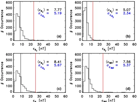
Fig. 3. Comparison of magnetic field vectors values estimated by

the geomagnetic model IGRF-11 + Tsy04 with values measured by

the FGM instrument. Panels (a), (b), (c) and (d) refer to thex,y,z

vector components and overall magnitude. Black vertical lines de-pict, respectively, the mean value of distributions displayed in each panel. Red vertical lines set the limit of rejected cases.

orbit configuration. It varies from year 2002, when the dis-tance is∼300 km three hours before perigee and∼250 km three hours after perigee, to year 2008, when the distances three hours before and after perigee amount to, respectively,

∼400 km and∼200 km.

2.3 Magnetic field coordinate system

To study how the electron density distribution is organised by the geomagnetic field lines, positions of electron density records are transformed into a geomagnetic coordinate sys-tem. From each position of observation,M, we follow the magnetic field line up to its apex,A, which defines the pa-rameter L (i.e. the geocentric distance of A, expressed in Earth-radii). MLat is the angle between geocentric vectors at apexA, and at positionM. MLT is defined by the mag-netic longitude at apexA. To do that, we need a robust ge-omagnetic model able to reproduce accurately all the vari-ability encompassed in the dataset. By comparing results of several geomagnetic models and FGM magnetic measure-ments, we chose to combine the IGRF-11 internal geomag-netic model (Finlay et al., 2010) with the Tsyganenko’s ex-ternal geomagnetic model version 2004, Tsy04 (Tsyganenko and Sitnov, 2005). These models have the advantage of be-ing constrained by a combination of geo-effective instanta-neous parameters (solar wind density and speed, magnitude of theByandBzcomponents of the interplanetary magnetic field and Dst index). By default, the values of these param-eters correspond to average interplanetary and ring current conditions. Moreover, Tsy04 considers the cumulative driv-ing of external sources on the magnetosphere, which allows reproducing a rapid evolution of the geomagnetic topology

Table 1. Contribution of each spacecraft to statistics, according to

analysed years.

Periods C1 C2 C3 C4

June 2002 to June 2003 121 131 120 0

January 2007 to December 2007 140 134 134 136

January 2008 to December 2008 110 129 99 0

January 2009 to April 2009 20 35 30 0

during unsteady conditions (an evolution ignored in the de-fault version of the model). This is an added value for the statistical analysis presented in this paper. It provides the ge-omagnetic coordinates of Cluster spacecraft at each element of the electron density profiles according to a realistic mag-netic topology and dynamics of the inner magnetosphere at the time resolution of measurements (about 1 min).

We retain density profiles for which the model reproduces accurately the FGM measured magnetic field. In order to do so, we calculate the mean absolute deviation (i)

be-tween modelled and measured values, over the magnetic field samples attached to the i-th density profile of our dataset (i =_N1 PNj=1kBjFGM−BjMODk, where j∈ [1, . . . , N],

Nis the number of bins ofi-th profile). This is calculated, re-spectively, for thex,y,zvector components of magnetic field and for its magnitude. Figure 3 shows the distribution of the mean absolute deviations (i). Black vertical lines indicate

the average of the mean absolute deviationshi. Whatever the magnetic field component, hi does not exceed 8.5 nT, which is about 1 % of the total magnetic field strength varia-tion recorded along a perigee pass. Tsy04 seems to improve slightly the accuracy of description in comparison with previ-ous versions of Tsyganenko’s model, like Tsy01, under quiet geomagnetic conditions (Woodfield et al., 2007; Zhang et al., 2010). Note also that, for each component (and for the mag-nitude), the standard deviation (σ) of the mean absolute de-viation is of the same order as the average value. This means that any component of the modelled magnetic field is statis-tically consistent with the measures. Despite the good accu-racy of the model, some perigee crossings stand out as out-liers. We reject them using the three sigma rule: if for one of the componentsi≥ hi +3σ, we reject thei-th profile (see

vertical red lines in Fig. 3). This is an objective criterion to discriminate perigee crossings for which geomagnetic condi-tions are not well enough reproduced.

2.0 4.0

6.0 8.0

10.0 -70-60-50

-40 -30

-20 -10

0 10 20 30 40 50 60 70

0 100 200 300 400 500 600 700 800

# Occurrence

2 4 6 8

10 03

06 09 12

15

18

21

24 0

100 200 300 400 500 600 700 800

# Occurrence

(a) (b)

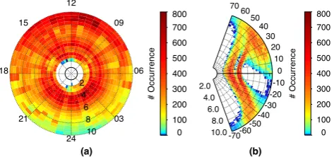
Fig. 4. Distribution of the electron density measurements gathered

after analysis of 1373 validated perigee passes. (a)L-MLT view of

the occurrence summed up inside magnetic flux tubes of section 0.5

inLand 0.5 h in MLT. (b)L-MLat view of the occurrence summed

up over all MLT sectors, for cells of dimension 0.2 inLover the

range 2 to 10 and 2.8◦in MLat over the range−70◦to 70◦.

The spatial distribution is almost uniform forLin the[3, 6]

interval, quasi uniform in the[6,8]interval, and not uniform in[2, 3]and in [8, 10]intervals. Note that occurrences of measurements are larger on the dayside than on the night-side. The dayside–nightside asymmetry results partly from the solar wind flow on the magnetosphere, which squeezes dayside magnetic field lines and stretches nightside magnetic field lines (as illustrated in Fig. 1). The region atL <10 is thus more frequently sampled in the dayside. Another factor is the duration of the second analysed period (1 January 2007 to 30 April 2009), which does not cover three full years and happens to favour the dayside MLT sectors. Finally, and this is likely the most important reason, nightside sectors are less populated than dayside ones (Carpenter and Ander-son, 1992). Consequently, the WHISPER instrumental limit is more often reached on the nightside of magnetosphere. The meridian projection (Fig. 4b) shows the latitudinal cov-erage over all MLT sectors. Note the presence of two arms due to the orbit drift effect. The outer arm (largerL-values at low latitude) corresponds to the first analysed period, i.e. 2002–2003, and the deeper one covering a larger interval inL-values near the equator corresponds to the 2007–2009 time period. In the Northern Hemisphere (MLat<50◦_{) and} for largeL-values (L≥8), another zone covered by Clus-ter appears. This zone corresponds to the observations made during the second crossing of the plasmasphere for perigee passes analysed after mid 2008.

3 Refilling process of the plasmasphere under quiet and steady magnetic activity

Our main objective in this section is to examine the plasma-sphere refilling process by presenting and discussing global density maps, sorted out according to magnetic activity con-ditions preceding measurements. Two main behaviours are expected during prevailing quiet magnetic activity: the

plas-masphere expansion up to largeL-values (co-rotation dom-inating in a region covering larger geocentric distances than prior to refilling), and the replenishment of flux tubes from their footprint at ionospheric altitudes to their apex. The two mechanisms are not independent, since a refilled plasmas-phere results from replenishment of flux tubes co-rotating in a region dominated previously by convection. The refill-ing of a magnetic flux tube from sunlit ionosphere has been modelled by assuming steady conditions at sources (Singh and Horwitz, 1992; Wilson et al., 1992). These models point to refilling durations which depend highly on the L-value considered, from approximately less than a day atL <4, to several days atL >6. Such durations are comparable to ob-served values quoted in Sect. 1.

Over long-term intervals, the ionospheric source linked to a magnetic flux tube in co-rotation is switched off in the night sector, which increases the overall refilling duration. The consequence of the equatorial drift pattern on the re-filling process is clearly illustrated by daily variations of the quiet plasmasphere density observed from the geosyn-chronous orbit (Reynolds et al., 2003). One can note that the dayside outer plasmasphere region is under replenishment quasi-permanently, whatever the fate of flux tubes when they reach the afternoon sector, co-rotation or sunward convection drift (D´ecr´eau et al., 1982). The dayside outer plasmasphere constitutes thus a reservoir of fresh cold plasma, a part of which can later be eventually aggregated to the main plas-masphere body.

3.1 Classification of density profiles

ap exceeds 15 nT, and being quiet otherwise. In practice, an entire density profile (all density records belonging to a given perigee pass) is sorted out as follows: we examine ap time series backward from the start time, starting from ap0 (at the time of the first density sample in the profile), and we note ap1 the first occurrence of ap exceeding the 15 nT limit. Let us call Dq the duration of the time sequence between ap1 and ap0, in unit of hours (Dq is a multiple of 3, and can be equal to 0). We sort out the density profiles in three classes, class 1 when Dq<48, class 2 when 48≤Dq<96, and class 3 oth-erwise (when Dq≥96).

In a second step, we examine the geomagnetic conditions attached to each density profile. Actually, selected density profiles are recorded over several hours, typically 8 to 10 h, wherein magnetic activity can change. We keep density pro-files for which ap index during the corresponding time in-terval does not exceed 15 nT, discarding thereby 243 density profiles (among them, the ones for which ap0>15 nT). Fol-lowing this selection, 575 density profiles belong to class 1, 245 to class 2 and 276 to class 3. All selected density profiles are acquired during quiet geomagnetic conditions, in the af-termath of an active event. In order to better appreciate what is the delay between the active event and the start of the den-sity profile, we have examined the distribution of Dq values in each class. Average delays are respectively less than a day (∼16 h) for the first class, about three days (∼70 h) for the second class, and more than six days (∼151 h) for the third class. The delays are distributed reasonably smoothly over the available intervals. In order to simplify the wording in the rest of the paper, we will refer to data of the first class as representative of the situation “after one day” (of quiet geomagnetic conditions), to the data of the second class as representative of the situation “after three days” and, finally, to the data of the third class as representative of the situation “after six days”.

Finally, let us recall that the classes defined above corre-spond to a long-term view of plasma evolution in the inner magnetosphere, in contrast with the short-term evolution of the magnetic field considered during the time interval of the density profile, as presented in Sect. 2.3. To our opinion, even if the density (the content) builds up in the long term, it is im-portant to survey the evolution of magnetic flux tubes (the container) in the short term, considering in particular that according to our selection criteria some density profiles are covered during moderate activity conditions such that the ge-omagnetic field configuration may vary significantly during the acquisition of the profile.

3.2 Global maps of density distribution

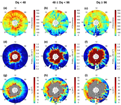
As indicated in Sect. 2.3, three magnetic field coordinates,L, MLT and MLat, have been attached to each density record by use of the magnetic field model tuned to the solar wind con-ditions related to the time of record. Figure 5 displays quanti-ties representative of the subset of density records measured

inside given magnetic flux tubes. The quantities are projected along field lines onto the magnetic equatorial plane, and pre-sented as a succession of equatorial maps, in the [2, 10]L -range, at a resolution of 0.5 inLand 0.5 h in MLT. This pro-cedure combines records taken in slightly different positions in physical space for a same L, MLT and MLat position, since the chosen magnetic field model is a dynamical one. However, it responds better to the concept of frozen-in field lines than a procedure using a static model would have.

Each column in Fig. 5 corresponds to one of the three classes defined in Sect. 3.1 above, from left to right: after one day, after three days and after six days of quiet geomag-netic conditions. Each row displays a different parameter, ex-tracted from everyL-MLT cell. The first parameter (panels a, b and c) is the number ofnemeasurements. The second one is the relative occurrence of densities above 80 cm−3_{, expressed} as a probabilityp(panels d, e and f). We arbitrarily assume that the density is above 80 cm−3 _{for all records with the} qualitative “high” density information (FUH>80 kHz). The third parameter is the median density value (panels g, h and i). We thus attribute the same weight to all density records along a given magnetic flux tube, as would be justified for a flat distribution in latitude. The cells coloured in grey in the bottom views represent the portion of the plasmasphere dom-inated by high-density values (median density value above 80 cm−3limit). This region matches exactly cells in the sec-ond row where the colour (from greenish to red) indicates a probability p greater than 0.5. The median parameter is more appropriate than the usual mean parameter to represent the density in aL-MLT cell since cells contain both quantita-tive information (density values) and qualitaquantita-tive information (namely that the density is above the 80 cm−3_limit).

Dq < 48

48 ≤ Dq < 96

(a)

(b)

(c)

(d)

(e)

(f)

(g)

(h)

(i)

2 4 6 8 10 03 06 09 12 15 18 21

24 0

10 20 30 40 50 60 70 80 ne [cm -3] 2 4 6 8 10 03 06 09 12 15 18 21

24 0

10 20 30 40 50 60 70 80 ne [cm -3] 2 4 6 8 10 03 06 09 12 15 18 21

24 0

10 20 30 40 50 60 70 80 ne [cm -3] 2 4 6 8 10 03 06 09 12 15 18 21

24 0.0

0.1 0.2 0.4 0.5 0.6 0.8 0.9 1.0 Prob[n e

> 80 cm

-3] 2 4 6 8 10 03 06 09 12 15 18 21

24 0.0

0.1 0.2 0.4 0.5 0.6 0.8 0.9 1.0 Prob[n e

> 80 cm

-3] 2 4 6 8 10 03 06 09 12 15 18 21

24 0.0

0.1 0.2 0.4 0.5 0.6 0.8 0.9 1.0 Prob[n e

> 80 cm

-3] 2 4 6 8 10 03 06 09 12 15 18 21

24 0

100 200 300 400 500 600 700 800 # Occurrence 2 4 6 8 10 03 06 09 12 15 18 21

24 0

100 200 300 400 500 600 700 800 # Occurrence 2 4 6 8 10 03 06 09 12 15 18 21

24 0

100 200 300 400 500 600 700 800 # Occurrence

Dq ≥ 96

Fig. 5. Electron density information inside magnetic flux tubes intersecting equatorial plane at a givenLand MLT are shown inL-MLT

views, using a resolution of 0.5 inLand 0.5 h in MLT. The first row shows the distribution of the occurrence ofnemeasurements in each

class. The second row displays the relative number of measured density values above 80 cm−3, expressed in terms of probability. The third

row displays the median value ofne. The electron density median is colour-coded on a linear scale and grey colour corresponds to the

portion of the plasmasphere dominated by high density values (>80 cm−3). The three columns display measurements obtained under the

three conditions defined in the study, namely 0≤Dq<48 (panels a, d and g), 48≤Dq<96 (panels b, e and h) and Dq≥96 (panels c, f

and i) of continuous quiet activity, where Dq is expressed in unit of hours.

to the outer limit of regions painted in grey in the bottom views of Fig. 5. In each category, the shape of the grey re-gion is representative of the shape of the plasmasphere in formation. It is roughly circular for the three data classes, with a radius increasing fromL∼4 in the first class (after one day of quiet conditions) toL∼6 in the second class (af-ter three days) andL∼[6.5, 7] in the third class (after six days). It appears thus that the main increase in theLsize of the plasmasphere occurs during the first three days of quiet

geomagnetic conditions, and that this size increases further after that, but slowly and slightly.

present in all sectors, up to highL-values (L∼8), except in the midnight sector where they are seen up toL∼5. The general shape drawn by median densities at ne=10 cm−3 (green to yellow colour code) is similar to the shape of the statistical outer boundary of measurable ions presented in Horwitz et al. (1990) (their Fig. 5a). A bulge of high den-sities (ne∼50 cm−3) shows up in the dusk sector (15:00– 21:00 MLT range). This is the region where, according to a classical interpretation, the co-rotation electric field and the convection electric field are equal and opposite (Carpen-ter, 1967; Chappell et al., 1970; Higel and Lei, 1984). Note also the local increase of the plasmapause-like boundary at 21:00 MLT (patch in grey colour up toL=6). This MLT sec-tor is where the bulge region is installed under very low ac-tivity (e.g. Carpenter, 1970; Maynard and Grebowsky, 1977). After 3 days of low activity (Fig. 5h), density values in the WHISPER range are observed in a large part of theL-MLT domain, with a smaller zone of very low density (dark blue) in the night sector than after one day. High-density values are present, irregularly, up to highL-values (L∼8 and above) in all MLT sectors. After six days of low activity (Fig. 5i), the presence of high densities up toL=8 and above is ob-served more systematically than for class 2, particularly in the 10:00–22:00 MLT sector.

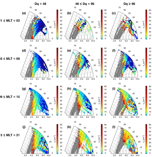
We examine now L-MLat maps of the median elec-tron density for the three classes of geomagnetic condi-tions defined above, and we present the results in Fig. 6, where each column corresponds to a given class. Four maps are elaborated with data from each class, group-ing density records acquired in four MLT sectors, respec-tively, around midnight (21:00≤MLT<03:00, first row), around dawn (03:00≤MLT<09:00, second row), around noon (09:00≤MLT<15:00, third row) and around dusk (15:00≤MLT<21:00, fourth row). Figure 6 is constructed in a similar way to Fig. 5: all density records from a dataset belonging to the selected class (of magnetic activity) and be-longing to a given cell inL and MLat value (of dimension 0.2 inLand 2.8◦in MLat, respectively) are grouped in a data packet, whatever their MLT value in the global sector consid-ered. Positive and negative latitudes are grouped in the same cell, assuming symmetry in term of density between both hemispheres. Indeed, density structures derived from a first

L-MLat mapping (not shown) appear as globally similar in each hemisphere. Joining data from both hemispheres allows a smooth coverage of a largeL-MLat zone covered partially in each hemisphere (see Fig.4b, showing theL-MLat orbital coverage). The question of inter-hemispheric symmetry will be investigated in the future. The median value of density in the data packet is shown using the same colour code as in Fig. 5, third row. Note that these views, like Fig. 4b, are presented in a different coordinate system than the famil-iar meridian views whereL-shells are drawing closed con-tours passing through the centre of the Earth (see for in-stance Laakso et al., 2002; Huang et al., 2004; Pierrard and Stegen, 2008). Here,L-shells are drawing geocentric circles

(L-values indicated on horizontal axes). Constant geocentric distance (dashed-dot curves), in the frame of a dipolar field assumption, are superimposed (R-values in Earth radii equal toL-values at equator).

One can distinguish three different zones in the maps of Fig. 6. The first one, coloured in grey, is characterised by densities above 80 cm−3. The second zone is characterised by densities in the WHISPER range (colour scale from blue to red). The third one is of a different nature. It is the blank zone, of variable extension in latitude, seen near the equator aroundL∼6. The latter zone is hidden in the maps of Fig. 5. It is due to a lack of orbital coverage, on the one hand (see Fig. 4b), and, on the other hand, to the presence of plasma of low density ignored in our dataset (explaining the larger blank zone in night side MLT sectors). Whatever their nature, the blank zones, covering regions at the apex of magnetic flux tubes where density values are likely lower than nearer to Earth, bias the statistical results shown in Fig. 5; some median densities plotted in this figure are overestimations of actual median densities.

The shape of the two first zones in the L-MLat maps presents characteristics forming novel information. The ex-tension of the first zone (high densities marked in grey colour) varies clearly with respect to the duration Dq of quiet magnetic activity, whereas there is no significant variation with the MLT sector considered. This is in agreement with the almost circular shape of the grey zone in the maps of panels (g) to (i) in Fig. 5. For the first class (after one day of low activity), maps of panels (a), (d), (g) and (j) in Fig. 6 display a grey zone occupying geocentric distances below

R∼3RE atL≥5 (note thatR is deduced from the con-version of theL-MLat position in geocentric distances, ac-cording to a simple dipolar model). BelowL∼5, the grey zone extends at higher geocentric distances, up toR∼4RE and even up to R∼5RE, in a patchy manner in the dusk sector and near the equator. The higher altitude of plasmas withne>80 cm−3inside anL-shell ofL∼5 (than outside) is an indication of a plasmasphere in formation. In this region (L <5) , a density decrease with decreasing magnetic lati-tude is visible forL >4, as happens on partially empty mag-netic flux tubes (Wilson et al., 1992), whereas atL <4 the information available in our dataset (median density larger than 80 cm−3) does not allow distinguishing partially empty from fully replenished flux tubes. For the second class of our dataset (after three days of low activity, panels b, e, h and k in Fig. 6), the grey zone occupies only geocentric distances below R∼3RE atL≥6. Inside anL-shell ofL∼6, the plasmas withne>80 cm−3extend at higher altitudes (up to

(f)

(a) (b) (c)

(d) (e)

21 ≤ MLT < 03

Dq < 48 48 ≤ Dq < 96

03 ≤ MLT < 09

(i)

(g) (h)

09 ≤ MLT < 15

(l)

(j) (k)

15 ≤ MLT < 21

2.0 4.0 6.0 8.0 10.0

0 10 20 30 40 50 60 70 0 10 20 30 40 50 60 70 80 ne [cm -3]

2.0 4.0 6.0 8.0 10.0 0 10 20 30 40 50 60 70 0 10 20 30 40 50 60 70 80 ne [cm -3]

2.0 4.0 6.0 8.0 10.0 0 10 20 30 40 50 60 70 0 10 20 30 40 50 60 70 80 ne [cm -3]

2.0 4.0 6.0 8.0 10.0

0 10 20 30 40 50 60 70 0 10 20 30 40 50 60 70 80 ne [cm -3]

2.0 4.0 6.0 8.0 10.0 0 10 20 30 40 50 60 70 0 10 20 30 40 50 60 70 80 ne [cm -3]

2.0 4.0 6.0 8.0 10.0

0 10 20 30 40 50 60 70 0 10 20 30 40 50 60 70 80 ne [cm -3]

2.0 4.0 6.0 8.0 10.0 0 10 20 30 40 50 60 70 0 10 20 30 40 50 60 70 80 ne [cm -3]

2.0 4.0 6.0 8.0 10.0

0 10 20 30 40 50 60 70 0 10 20 30 40 50 60 70 80 ne [cm -3]

2.0 4.0 6.0 8.0 10.0 0 10 20 30 40 50 60 70 0 10 20 30 40 50 60 70 80 ne [cm -3]

2.0 4.0 6.0 8.0 10.0

0 10 20 30 40 50 60 70 0 10 20 30 40 50 60 70 80 ne [cm -3]

2.0 4.0 6.0 8.0 10.0

0 10 20 30 40 50 60 70 0 10 20 30 40 50 60 70 80 ne [cm -3]

2.0 4.0 6.0 8.0 10.0 0 10 20 30 40 50 60 70 0 10 20 30 40 50 60 70 80 ne [cm -3]

Dq ≥ 96

Fig. 6.L-MLat views of the median value of densities measured at a givenL-shell and magnetic latitude (defined in absolute value) using

a resolution of 0.2 inLand 2.8◦in MLat. Datasets combine density records over large local time sectors, 21:00–03:00 MLT (first row),

03:00–09:00 MLT (second row), 09:00–15:00 MLT (third row) and 15:00–21:00 MLT (fourth row). The three columns are defined as in

Fig. 5. Colour codes are defined as in Fig. 5, second row. Iso-Rcurves, whereRis the geocentric distance derived from theL-MLat position,

according to the dipolar model, are also superimposed (dashed-dot lines) in order to guide the reader.

of this behaviour. Finally, the third class of our dataset (after six days, panels c, f, i and j in Fig. 6) displays similar char-acteristics: a plasmasphere in formation inside a still higher

L-shell (L≥6.5).

09 MLT

<

15 5.5

<

L 6.5

1 10 100

ne

[cm

-3 ]

0.0 0.2 0.4 0.6 0.8 1.0

Prob[n

e

>

80 cm

-3 ]

0 10 20 30 40 50 60 70

|MLat | 10

100 1000

# Occurrence

Dq < 48 48 Dq < 96 Dq 96

(a)

(b)

(c)

Fig. 7. Distribution of electron density versus latitude (at a

resolu-tion of 2◦), for magnetic flux tubes covering the 09:00–15:00 MLT

sector and crossing magnetic equator at 5.5≤L <6.5. Panel (a)

displays the scatter plot ofnerecords (dots) and the

correspond-ing median values (full circles). Panel (b) displays the probability

of observing densities greater than 80 cm−3 and panel (c) shows

occurrence numbers. For all panels, the three curves depict

prop-erties ofnefor a duration of quiet activity being Dq<48 (blue),

48≤Dq<96 (black) and Dq≥96 (red), as defined in the text.

maps display a clear evolution of this zone, not only with the duration Dq (i.e. a displacement with Dq, which is a conse-quence of the spatial extension of the first zone with Dq) but also an evolution with the MLT sector considered. The MLT dependence for the first class of magnetic activity (maps in the left column) is two fold: (i) the boundary layer, i.e. the zone coloured from red to green, narrows in the midnight sector (Fig. 6a), and gets thicker and thicker with increas-ing central MLT (panels d, g and j in Fig. 6); (ii) a zone with patchy cells at high densities (red or yellow colour) is present above a geocentric distanceR∼6REin the noon and dusk

sectors (panels g and j, Fig. 6), whereas the midnight and dawn sectors (panels a and d, Fig. 6) indicate densities either low (blue colour) or not measurable (blank zone) in this area. For the second and third classes of activity (maps shown, re-spectively, in the central and right columns of Fig. 6), one can note the presence of small regions of high or medium densities in the night and dawn sectors at high altitudes and highL-values (R >6RE,L >7), which are not seen in the left column. The patchy cells of high or medium densities cover a larger area in the noon and dusk sectors than in the night and dawn sectors (panels h, i, k and l compared to pan-els b, c, e and f in Fig. 6). Moreover, the noon and dusk sectors display a large area of intermediate densities (yellow to red colours) at high magnetic latitudes and L-values. In summary, both the “plasmasphere” (ne>80 cm−3) and the neighbouring “trough” (nein the WHISPER range) expand in volume with the duration of low activity, and mainly in the noon and dusk sectors. Our dataset does not cover all key ar-eas of theL-MLat map but it seems that, even after six days, the apex of flux tubes is still partially empty aboveL∼6.

3.3 Detailed density distribution along magnetic flux tubes and near equatorial plane

We now present further details of the density distribution, shown in Figs. 7 to 9, where individual measured density values are visible. This allows the dispersion of the measured densities to be appreciated around the median values calcu-lated inside chosen cells of theL– MLat – MLT domain. Fig-ure 7a presents the distribution of density values (thin dots) covering the sector 09:00–15:00 in MLT and the range 5.5 to 6.5 inL-values, as a function of the magnetic latitude MLat, for the three classes of magnetic activity history. The reso-lution in MLat is 2◦. A given colour code attributed to each class allows a direct comparison of the median density values (thick dots), with same values presented (at a better resolu-tion inL) in theL-MLat panels (g) to (i) in Fig. 6. Figure 7 displays also the percentage of observation above 80 cm−3 limit (panel b) and the total number of density records in each data subset (panel c).

Above about 45◦MLat, all three classes show the same characteristics: a majority of density values above 80 cm−3, and a similar total number of records. Between 35◦and 45◦ latitude, the number of records is significant in all classes and the percentage of high values increases with increasing refill-ing duration. This behaviour is consistent with a view where the total content of a flux tube increases with the duration of refilling. It indicates that, aroundL=6, the refilling pro-cess is still active after three quiet days. Below 30◦MLat, the probabilitypfor class 3, as well as the density profile, dis-play an irregular behaviour, which is likely due to the small number of records.

quantitative features which can be compared to published models and observations. For the first class of data, the scat-ter plot is reasonably compact around median density values. The latitudinal profile of median densities draws a concave shape, qualitatively similar to what is obtained in a colli-sional kinetic models, after the first hours of refilling of ini-tially empty flux tubes, and during the subsequent time in-terval, when ions diffuse via collisions (Wilson et al., 1992). Near the equator, the profilene(MLat)is almost flat, then the slope increases with MLat, presenting a step-like shape in the range [35◦, 45◦]. The median value obtained at the lowest latitude available (15◦) isne∼8 cm−3, equal to the density calculated at L=6 with the above quoted model. This value is also comparable to values observed on board ISEE in the dayside trough (Carpenter and Anderson, 1992), i.e. ne in the [4, 9] cm−3 interval. For the second class of data (after three days), the number of density records near the equator (MLat<20◦_{) is too scarce for median values to} be discussed quantitatively. In the [20◦, 25◦] MLat interval, median values (in the [20, 60] cm−3interval) are comparable to the value of 30 cm−3obtained in the model of Wilson et al. (1992) at the equator after a refilling duration of 48 h. Finally, the median value obtained at MLat=30◦for the third class (after six days) is greater than 80 cm−3, which complies with the equatorial densitiesne∼100 cm−3observed atL=6 in the dayside saturated plasmasphere (Carpenter and Ander-son, 1992). More generally, the density values belonging to class 2 and class 3 are similar to values obtained by in situ or whistler observations after an extended quiet period (Corcuff et al., 1972), while the density values belonging to class 1 correspond to density values characteristic of the permanent dayside reservoir (D´ecr´eau et al., 1982).

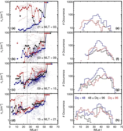
Figure 8 displays the same quantities as shown in Figs. 7a and 7c, but for higher L-values, i.e. 7.5< L <8.5, and in four MLT intervals covering all MLT sectors. Scatter plots and median values are displayed on the left side of the figure, and matching occurrences on the right side. Suc-cessive MLT sectors are displayed from top to bottom, with increasing hours: 21:00–03:00 MLT, 03:00–09:00 MLT, 09:00–15:00 MLT and 15:00–21:00 MLT. At high latitudes (MLat>50◦), the density profiles are only indicative. In-deed, the gyrofrequency is important and the qualitative den-sity information (densities placed at ne=80 cm−3 in the scatter plot) is not reliable (see Sect. 2.1).

The density variations versus MLat shown in Fig. 8c can be compared to the density profiles shown in Fig. 7, top panel. This allows the result of the refilling process to be appreciated in the same MLT sector, but along magnetic flux tubes at two differentL-values. For the first class of magnetic activity (blue curves), the two profiles are qualitatively simi-lar: almost flat near the equator, they display a larger slope in density at high latitudes, above, respectively, at MLat∼40◦ for L∼6 (Fig. 7) and at MLat∼50◦ for L∼8 (Fig. 8). These magnetic latitudes, when converted in geocentric dis-tances – using the Tsyganenko model shown in Fig. 1 –

lead to similar geocentric distances of, respectively, 3.6RE (L=6) and 4.0RE(L=8). Quantitatively, the median den-sity near the equator isne∼2 cm−3atL∼8 (compared to

ne∼8 cm−3atL∼6), in agreement with the “trough” equa-torial density value published by Carpenter and Anderson (1992). Median densities increase with the duration Dq of low activity, but in a less spectacular way than at L∼6. Among the very dispersed values seen in the scatter plot of data belonging to class 3 (red dots, Fig. 8c), the highest ones,

ne∼40 cm−3(at MLat∼20◦), are comparable to the highest densities encountered by ISEE 1 in the dayside “saturated” plasmasphere near the equator, atL=8 (Carpenter and An-derson, 1992).

More generally, the density distribution displayed in all four MLT sectors of Fig. 8 can be described as follows:

1. Two main types ofne(MLat)profiles are showing up. The first type, which we will refer to as a “trough” like profile (for example, all median densities in class 1), displays a concave shape, shallow near the equator. The second type, which we will refer to as a “saturated plas-masphere” like profile, displays a flat shape. It is formed by the highest density values in MLat bins of the scatter plots of class 3. These two types reproduce modelled behaviours, respectively, in partially empty flux tubes and in saturated flux tubes (Wilson et al., 1992); 2. Trough like profiles display density values increasing

with MLT sectors presented from top to bottom panels. At MLat=30◦, densities from smoothed profiles are, respectively, 0.9 cm−3_{in the midnight sector, 1.5 cm}−3 in the dawn sector, 2.5 cm−3 _{in the noon sector, and} 5 cm−3_{in the dusk sector. In contrast, densities in} “sat-urated profiles” cannot be valuably compared from one MLT sector to the next. All of them display similar val-ues (ne∼60 cm−3), more than an order of magnitude above trough values;

3. When the occurrence of measurement is sufficient to compare median densities of the three different classes, the increase of density with the duration Dq is modest. An increase of the order of a factor two after several days can be noted at MLat=45◦_{(panels b, c, d);} 4. The huge dispersion of density values in a same MLT –

L– MLat cell, for the three classes of magnetic activ-ity, indicates that the chosen criteria for sorting out the dataset is not very efficient. More selective criteria, for instance choosing a smaller ap value to define low activ-ity, could be worked out. As an example, the high den-sities measured in the night sector (Fig. 8a) correspond to an event (15 November 2008) with ap≤4 during five consecutive days;

1

10

100

n

[cm

-3

]

21 MLT < 03

₁₀

100

1000

# Occurrence

1

10

100

n

[cm

-3

]

03 MLT

<

09

₁₀

100

1000

# Occurrence

1

10

100

n

[cm

-3

]

09 MLT < 15

₁₀

100

1000

# Occurrence

0

10

20

30

40

50

60

70

|MLat |

1

10

100

n

[cm

-3

]

15 MLT < 21

0

10

20

30

40

50

60

70

|MLat |

10

100

1000

# Occurrence

Dq

<

48

48 Dq < 96

Dq 96

(a)

(b)

(c)

(d)

(e)

(f)

(g)

(h)

Fig. 8. Same as Fig. 7a (left column) and Fig. 7c (right column), but for field lines at higherL-values, 7.5≤L <8.5. Scatter plot (left) and occurrence numbers (right) are split in four MLT sectors, as in Fig. 6: 21:00–03:00 MLT (panels a and e), 03:00–09:00 MLT (panels b and

f), 09:00–15:00 MLT (panels c and g) and 15:00–21:00 MLT (panels d and h).

The objective of Fig. 9 is to visualise equatorial density pro-files,ne(L), after different refilling durations, and over four MLT sectors, using the same presentation as Fig. 8. Left panels display scatter plots and median densities at a res-olution of 0.25 inL, and right panels display occurrences.

1

10

100

n

[cm

-3

]

21 MLT

<

03

₁₀

100

1000

# Occurrence

1

10

100

n

[cm

-3

]

03 MLT

<

09

₁₀

100

1000

# Occurrence

1

10

100

n

[cm

-3

]

09 MLT

<

15

₁₀

100

1000

# Occurrence

0

2

4

6

8

10

L

1

10

100

n

[cm

-3

]

15 MLT

<

21

0

2

4

6

8

10

L

10

100

1000

# Occurrence

Dq < 48

48 Dq

<

96

Dq 96

(a)

(b)

(c)

(d)

(e)

(g)

(h)

(f)

Fig. 9. Distribution of electron density versusL, using a resolution of 0.25 inL-value, over a region covering the latitudinal range−30◦≤

MLat≤30◦. Panels display identical quantities as in Fig. 8, using the same colour code. Dashed lines show distributions inL−4.

carry the same plasma content (noting that their volume vary asL−4).

The plots shown in Fig. 9 confirm the observed evolution of density withL-value described above: (i) a clear increase of density with the duration Dq of low activity forL-shells in the lower range (4< L <6) and a smaller increase in the

remarks concern the signature of a plasmapause like bound-ary, i.e. a density step in the profilene(L). This step disap-pears in the dusk sector. This could indicate that, under con-ditions of low activity, equatorial drift paths are closed up to highL-values. In the three other MLT sectors, this step shows up clearly. Its position in L increases with the du-ration Dq of low activity. There is no clear dependence of this boundary according to the MLT sector, a feature already mentioned above, in the descriptions of Figs. 5 and 6. Further remarks concern density values in the noon and dusk sector. They are placed inside a slice bounded by two profiles in

L−4. The lowest values are probably controlled by the day-side reservoir (D´ecr´eau et al., 1982), and the highest values by the total volume available inside magnetic flux tubes. In contrast, very low densities are observed in the nightside of the magnetosphere (Fig. 9a).

3.4 Discussion

The paradigm we wish to examine here is how, under con-ditions of a globally stationary equatorial convection pattern (ap≤15 nT after episodes with ap>15 nT), the volume of a plasmasphere in formation is getting replenished. This vol-ume is assvol-umed, in a simple picture, to be rigidly bounded (by the last closed equatorial drift path and its projection along magnetic field lines forming a “final” PBL) and at least partially emptied from erosion mechanisms. Supplies (and losses) of matter, at ionospheric level, are expected to bring (or remove) plasma material inside this volume, sup-plies being on average more effective than losses. Having no preconception about the position of the final PBL, we exam-ine the density distribution over the global volume inside a largeL-range[2, 10]. The general questions we wish to ad-dress, and try to answer from our density observations, are the following: What is the final shape of the plasmasphere in formation? How does the ionized gas occupy the three-dimensional space available? Our ambition, at the same time, is to try and improve our understanding of the physics of the plasmasphere refilling process. We shall now examine our results according to three different aspects of the question addressed above, in turn.

3.4.1 Final boundary of the plasmasphere in formation

TheL-MLT maps in Fig. 5 display the shape of an “instan-taneous” PBL (the outward limit of the grey zone), which expands with the duration Dq (see Sect. 3.2). This quasi-circular PBL expands of about 2REin two days, and of about 0.5RE during the next three days, which could lead to the interpretation that a “final” boundary, approached asymptot-ically, is placed next to the largest observed PBL, i.e. at a ra-dius of about 7RE. However, observations presented later in the paper demonstrate that this view is oversimplified. They demonstrate (i) that the volume inside the L=7 magnetic shell is far from being filled up to saturation, at least on

av-erage, after the longest Dq value considered (Figs. 6 and 9); and (ii) that some events display saturated latitudinal density profiles atL∼8 (Fig. 8) after five very quiet days. We con-sider, thus, that we must revise the paradigm stated above. It is likely valid for a selection of events present in our dataset but there is not a large enough number of these to allow the 3-D analysis aimed at. For most of our selected events, the equatorial convection pattern is not stationary, and the “final” boundary is a moving one. As a consequence, our statistical analysis of the 3-D refilling pattern is to be taken as repre-sentative of a refilling plasmasphere where plasma losses are not only occurring at ionospheric levels but also at higher al-titudes from plasmasphere erosion during episodes of mod-erate activity.

The effects of a centrifugal force due to co-rotation of the plasma with the angular velocity of the Earth had been brought to attention by Lemaire (1974) as an important mechanism leading to plasmasphere erosion in the dawn sec-tor atL <5.8 (Pierrard and Cabrera, 2005). Erosion is due to convective instability inducing interchange motion of flux tubes transverse to equatorial drift paths. Recently, Andr´e and Lemaire (2006) have shown that effects of the mag-netic curvature on convective instability, when taken into account, are largely dominant over the effects of the effec-tive gravity in the equatorial regions of the plasmasphere. They show that, in addition to transverse interchange mo-tion, translational (along field lines) interchange motion is to be expected. They have shown in particular that the density model derived empirically for a saturated plasmasphere by Carpenter and Anderson (1992), is unstable aboveL=6.6. More generally, Andr´e and Lemaire (2006) demonstrate that the plasmaspheric wind is a leakage mechanism active deep inside the plasmasphere. In brief, this recent study provides important hints about physical mechanisms controlling the refilling process of the plasmasphere under realistic condi-tions, stressing the importance of a 3-D picture.

3.4.2 Latitudinal distributions