Modeling ionospheric fo F2 by using empirical orthogonal function analysis

www.ann-geophys.net/29/1501/2011/ doi:10.5194/angeo-29-1501-2011

© Author(s) 2011. CC Attribution 3.0 License.

Annales

Geophysicae

Modeling ionospheric foF2 by using empirical orthogonal function

analysis

E. A1,2, D.-H. Zhang1,3, Z. Xiao1,3, Y.-Q. Hao1, A. J. Ridley2, and M. Moldwin2

1_{Institute of Space Physics and Applied Technology, School of Earth and Space Sciences, Peking University, Beijing, China} 2_{Department of Atmospheric, Oceanic and Space Sciences, University of Michigan, Ann Arbor, MI, USA}

3_{State Key Laboratory of Space Weather, Chinese Academy of Sciences, Beijing, China}

Received: 12 April 2011 – Revised: 11 August 2011 – Accepted: 26 August 2011 – Published: 31 August 2011

Abstract. A similar-parameters interpolation method and an

empirical orthogonal function analysis are used to construct empirical models for the ionospheric foF2 by using the obser-vational data from three ground-based ionosonde stations in Japan which are Wakkanai (Geographic 45.4◦N, 141.7◦E), Kokubunji (Geographic 35.7◦N, 140.1◦E) and Yamagawa (Geographic 31.2◦N, 130.6◦E) during the years of 1971– 1987. The impact of different drivers towards ionospheric

foF2 can be well indicated by choosing appropriate

prox-ies. It is shown that the missing data of original foF2 can be optimal refilled using similar-parameters method. The characteristics of base functions and associated coefficients of EOF model are analyzed. The diurnal variation of base functions can reflect the essential nature of ionospheric foF2 while the coefficients represent the long-term alteration ten-dency. The 1st order EOF coefficientA1can reflect the fea-ture of the components with solar cycle variation. A1 also contains an evident semi-annual variation component as well as a relatively weak annual fluctuation component. Both of which are not so obvious as the solar cycle variation. The 2nd order coefficient A2 contains mainly annual variation components. The 3rd order coefficientA3and 4th order co-efficientA4contain both annual and semi-annual variation components. The seasonal variation, solar rotation oscilla-tion and the small-scale irregularities are also included in the 4th order coefficientA4. The amplitude range and develop-ing tendency of all these coefficients depend on the level of solar activity and geomagnetic activity. The reliability and validity of EOF model are verified by comparison with ob-servational data and with International Reference Ionosphere (IRI). The agreement between observations and EOF model is quite well, indicating that the EOF model can reflect the major changes and the temporal distribution characteristics

Correspondence to: D.-H. Zhang

([email protected])

of the mid-latitude ionosphere of the Sea of Japan region. The error analysis processes imply that there are seasonal anomaly and semi-annual asymmetry phenomena which are consistent with pre-existing ionosphere theory.

Keywords. Ionosphere (Modeling and forecasting)

1 Introduction

Different types of variability in ionosphere are subject to a number of interconnecting drivers which can be broadly characterized as follows: (a) solar ionizing radiation; (b) ge-omagnetic activity; and (c) meteorological influences (e.g., Forbes et al., 2000; Rishbeth and Mendillo, 2001; Lei et al., 2008b; Zhang et al., 2011). The ability to model and eventu-ally anticipate the solar cycle, annual, semi-annual and sea-sonal variations as well as irregularities in ionosphere is of great use for both ionospheric research and space weather applications (T´oth et al., 2005). An ionospheric model can be either a first-principles-based physics model which is developed from a rigorous mathematical analysis of laws of physics and based on numerical solution of the spatial-temporal equations, or an empirical model which refers to any kind of modeling based on empirical observations. The empirical ionospheric model, which usually describes the spatial and temporal variation of electron density, critical fre-quency, electron temperature and other parameters of iono-sphere in the form of various types of functions (e.g., har-monic function, Chapman function), played an important part in extensive practical applications.

Table 1. Geographic and geomagnetic positions of the ionosondes

in Japan.

Station Geographic Geographic Geomagnetic name latitude (◦N) longitude (◦E) latitude (◦N)

Wakkanai 45.4 141.7 35.4

Kokubunji 35.7 139.5 25.6

Yamagawa 31.2 130.6 20.4

frequencies. The relationship of peak density NmF2 (unit: m−3) and foF2 (unit: MHz) is as follows.

NmF2=1.24×1010×(foF2)2 (1)

Therefore, the F2 layer critical frequency foF2 is one of the most significant ionospheric parameters from which the morphology of topside density profile can be well charac-terized. IRI provides two choices to describe the foF2: CCIR (International Radio Consultative Committee) or now known as ITU (International Telecommunication Union) model (CCIR, 1967), and URSI (International Union of Ra-dio Science) model (Rush, 1992). Both cases are based on the observations from the worldwide network of ionosonde stations. The availability of reliable data for the specific re-gion and time determined the accuracy of the model (Bilitza and Reinisch, 2008). The ionosphere in East Asia is an im-portant region where the station density is relatively dense. However, the electro and atmospheric dynamics within mid-dle and low latitude ionosphere of East Asia region which is controlled by the equatorial anomaly phenomena can be very complicated. Several studies have shown that there are rel-atively large discrepancies between the ionospheric param-eters predicted by IRI model and the observational data in equatorial and low latitude regions, especially in East Asia and southern China area (Adeniyi et al., 2003; Liu et al., 2004; Zhang et al., 2004). Zhang et al. (2007) examined that the percentage difference values of foF2 predictions by us-ing URSI coefficients in IRI pattern can reach as large as 30 % around pre-sunrise time, and between −5 % percent and−25 % during most time period of the day. Therefore, it is necessary to update the existing CCIR or URSI foF2 model or build directly a single station or regional model of

foF2 among East Asia region.

Several new modeling techniques with respect to differ-ent ionospheric parameters have been proposed. Some stud-ies made the temporal and spatial forecasting of ionospheric

foF2 and built the model by using neural network analysis

(Kumluca et al., 1999; Oyeyemi et al., 2005, 2006; McKin-nell and Oyeyemi, 2009, 2010). Of particular intention is concentrated on modeling the ionospheric parameters such as foE, foF2, hmF2, and M(3000)F2, etc. based on empiri-cal orthogonal function analysis (e.g., Dvinskikh, 1988; Liu et al., 2008; Zhang et al., 2009). In this paper, we will fo-cus on constructing single station model of ionospheric foF2

for Wakkanai (Geographic 45.4◦_{N, 141.7}◦_{E), Kokubunji}

(Geographic 35.7◦_{N, 140.1}◦_{E) and Yamagawa (Geographic}

31.2◦_{N, 130.6}◦_{E) during the years of 1971–1987 by using}

similar-parameters interpolation method and empirical or-thogonal analysis, and the results are compared with the ob-servational data and with IRI model.

2 Data set for station modeling

The ionospheric F-layer over Japan, which lies near the inner flank of the northern crest of ionospheric equatorial anomaly, is a representative sector of East Asia (geographic longitude range: 130◦E–145◦E; geographic latitude range: 30◦ N-45◦N; geomagnetic latitude range: 18◦N–35◦N). Relatively large discrepancies have been measured between IRI and ob-servational values among this sector (Liang, 1990; Adeniyi et al., 2003; Bilitza et al., 2006; Vlasov and Kelley, 2010). Here we use hourly foF2 data observed at three ground-based ionosonde stations in Japan which are Wakkanai, Kokubunji and Yamagawa. These three stations are the oldest estab-lished ionosonde sites with long history of reliable data of ionograms (Xu et al., 2004; Lei et al., 2008a). The time pe-riod of 1971–1987 are used in the present study because it covers more than one whole solar cycle as long as possible with the maximum data availability. The ionosonde data for 1980, 1981 (high solar activity years) and 1986, 1987 (low solar activity years) are used for data-model comparison in order to assess to what degree the empirical model can repre-sent the observational results. The geographical coordinates and geomagnetic latitudes are listed in Table 1.

3 Description of the similar-parameters interpolation

method

We use similar-parameters method to refill the missing data for aforementioned three stations during the time period of 1971–1987. Similar-parameters method, which was origi-nally applied to the field of aerodynamics (see NASA web-site: http://www.grc.nasa.gov/WWW/k-12/rocket/airsim), can be used to interpolate the missing data before construct-ing the empirical model. In this method, the observational data can be influenced and determined by all possible factors or parameters. If two data sets have the same values for the similarity parameters, the data set which contains the miss-ing value under certain temporal and spatial conditions can be interpolated by using its “control” data set. Here we list several possible drivers of ionospheric variability of F layer in Table 2.

Table 2. Possible drivers of ionospheric variability of F layer.

Solar ionizing radiation Geomagnetic activity Meteorological influences

Solar cycle variation Magnetic storms Solar and lunar tides Solar rotation variation Substorms Acoustic and gravity waves Seasonal variation IMF/Solar wind Planetary waves

Solar flares Energetic particle precipitation Lower atmosphere influence

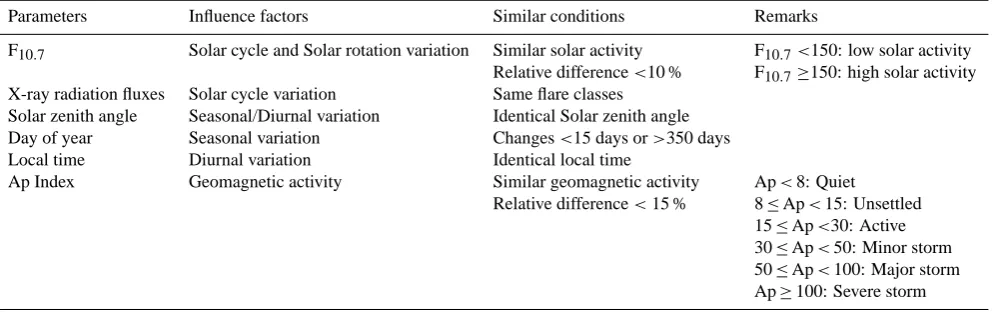
Table 3. The settings of the similar parameters.

Parameters Influence factors Similar conditions Remarks

F10.7 Solar cycle and Solar rotation variation Similar solar activity F10.7<150: low solar activity Relative difference<10 % F10.7≥150: high solar activity X-ray radiation fluxes Solar cycle variation Same flare classes

Solar zenith angle Seasonal/Diurnal variation Identical Solar zenith angle Day of year Seasonal variation Changes<15 days or>350 days Local time Diurnal variation Identical local time

Ap Index Geomagnetic activity Similar geomagnetic activity Ap<8: Quiet Relative difference<15 % 8≤Ap<15: Unsettled

15≤Ap<30: Active 30≤Ap<50: Minor storm 50≤Ap<100: Major storm Ap≥100: Severe storm

The solar radiation also related to the change in X-ray radia-tion fluxes which also need to be set as proxy. The seasonal variation is related to change in solar zenith angle which is a function of DOY (day of year), local time and latitude. As the latitude is fixed for single station, here we choose DOY (day of year) and local time as proxies. For the geomagnetic activity, Ap index is a suitable proxy because it is a plan-etary index for calculating the strength of world-wide geo-magnetic disturbances. For the meteorological influences, Mendillo et al. (1998) tried to estimate to what degree the F-layer variability could be attributed to the troposphere and lower stratosphere by using the NCAR (National Cen-ter for Atmospheric Research) coupled CCM3/TIME-GCM (Community Climate Model-3/Thermospere-Ionosphere-Mesosphere-Electrodynamics General Circulation Model; Roble and Ridley, 1994). Mikhailov et al. (2007, 2009) showed that synchronous variation of electron density can be observed during geomagnetic quiet day in both E- and F-region. Such variability is considered to be caused by per-turbation originating from lower atmosphere. It is hard to set appropriate proxy for meteorological influences not only be-cause the major influences to the variation of foF2 are due to solar ionizing and geomagnetic activity but also since there are so many uncertainties in the climate change as well as in the generation and transmission of the wave. Therefore, the parameters being used here are F10.7, Ap index, local time and DOY based on aforementioned analysis. At any single station, the missing value can be interpolated by choosing

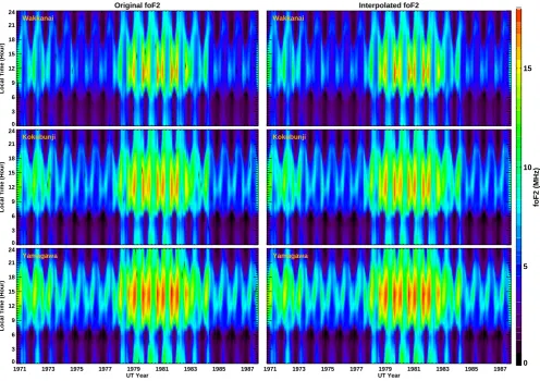
the median value from the data set which have the “simi-lar” parameters. The settings of the similar parameters are listed in Table 3. One thing worth noting is that the any in-terpolation method cannot be a good one for interpolating long-gap missing data. However, the data missing for foF2 at Wakkanai, Kokubunji, and Yamagawa during the time in-terval 1971–1987 is only scattered, which makes it possible to implement the interpolation method. Figure 1 displays the comparison of the original and interpolated foF2 values. It can be seen from the figure that the similar-parameters inter-polation method is fairly feasible for data preprocessing.

4 Description of the modeling technique

4.1 Brief introduction of EOF analysis method

Original foF2

24

21

18

15

12

9

6

3

0

Local Time (Hour)

Wakkanai

Interpolated foF2

Wakkanai

24

21

18

15

12

9

6

3

0

Local Time (Hour)

Kokubunji Kokubunji

1971 1973 1975 1977 1979 1981 1983 1985 1987

UT Year 24

21

18

15

12

9

6

3

0

Local Time (Hour)

Yamagawa

1971 1973 1975 1977 1979 1981 1983 1985 1987

UT Year Yamagawa

0 5 10 15

foF2 (MHz)

Fig. 1. Comparison among the original foF2 (left panels) and interpolated foF2 using similar-parameters method during the interval 1971–

1987 at three ionosonde stations.

are attributed to different factors which can be extracted and separated in terms of their relative “contribution” with re-spect to ionospheric parameters. The EOF method can be utilized to decompose and express the variation as a sum-mation of the eigen modes which are not pre-specified arti-ficially, but are calculated according to experimental data it-self in the decomposition process. The combination of eigen modes can reproduce the substantive characteristics of the data. The eigen series have rapid convergence velocity and high calculation accuracy. This makes EOF analysis method a highly effective way of empirical modeling not only by greatly reducing the modeling parameters but also by con-siderably saving the computation time compared with other expansion methods. For further details of EOF decomposi-tion, readers may refer to Dvinskikh (1988), Xu and Kamide (2004), and Zhang et al. (2009).

4.2 Data processing with EOF analysis method

The hourly values of foF2 at three stations are decom-posed into the EOF base functions Ek, multiplied by the

corresponding EOF coefficientsAk using the EOF analysis

method:

foF2(d,h)=

24 X

k=1

Ek(h)×Ak(d) (2)

Where foF2(d, h) is the combination of hourly values of the observational data expressed as a 6209×24 array with the rows corresponding to the days (d=1,2,3...,6209) which is calculated from 1 January 1971; The column correspond-ing to the local time LT(h=0,1,2...,23). Ek(h)is thek-th

base function of foF2 reflecting the diurnal variation,Ak(d)

is the coefficients of Ek(h) which represents the long-term

0.10 0.15 0.20 0.25 0.30

E1

Wakkanai _E1

foF2

4 6 8 10

foF2 (MHz)

-0.6 -0.4 -0.2 -0.0 0.2 0.4 0.6

E2

Wakkanai Kokubunji Yamagawa

0.10 0.15 0.20 0.25 0.30

E1

Kokubunji _E1

foF2

4 6 8 10

foF2 (MHz)

-0.6 -0.4 -0.2 -0.0 0.2 0.4 0.6

E3

Wakkanai Kokubunji Yamagawa

0 3 6 9 12 15 18 21 24 Local Time (Hour)

0.10 0.15 0.20 0.25 0.30

E1

Yamagawa _E1

foF2

4 6 8 10

foF2 (MHz)

0 3 6 9 12 15 18 21 24 Local Time (Hour)

-0.6 -0.4 -0.2 0.0 0.2 0.4 0.6

E4

Wakkanai Kokubunji Yamagawa

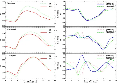
Fig. 2. Diurnal variation of the first EOF base functions and the foF2 (left panels) and 2nd to 4th order base functions (right panels) at three

stations.

fluctuation of the original data matrix, are used to reconstruct the foF2 and build the model. So it is feasible to reduce the number of modeling parameters and to simplify the calcu-lating process to a great extent while the accuracy of data reconstruction being considerably high.

Figure 2 shows the diurnal variation of the first four or-der EOF base functions and the foF2 at three stations re-spectively. It can be clearly seen from the left panels that the diurnal variation of the 1st order base functionE1 and

foF2 are quite similar to each other, the correlation

coeffi-cients betweenE1and foF2 are greater than 0.97 among all those three stations. ThereforeE1 can represent the aver-age diurnal variation trend of foF2. The ionospheric foF2 is also influenced by other factors which including interhemi-spheric flow, neutral winds and diffusion. Thus one would expect there are small scale disturbances and irregularities superimposed on the diurnal variation due to above influ-ences, which are well represented from the variation of the 2nd, 3rd and 4th order base functions in the right panels. Take the 3rd order base functionE3as an example. E3

be-gins to increase at around 05:00 ˙LT and then has a decreasing trend at around 11:00 LT and increases again from 17:00 LT. These phenomena can be explained by ionospheric sunrise enhancement, bite out phenomena and sunset enhancement respectively (Schunk and Nagy, 2000; Liu et al., 2004).

0 20 40 60 80

A1

Wakkanai

A1 F107

100 150 200

F107

0 20 40 60 80

A1

Kokubunji

A1 F107

100 150 200

F107

1971 1973 1975 1977 1979 1981 1983 1985 1987

UT Years 0

20 40 60 80

A1

Yamagawa

A1 F107

100 150 200

F107

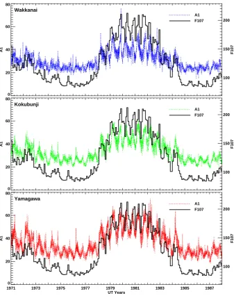
Fig. 3. Long-term variation of F10.7and the 1st EOF coefficients from 1971–1987.

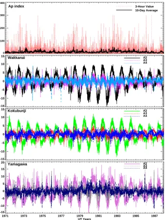
The synchronous solar cycle variation trends both inA1 and in F10.7 for all three ionosonde stations can reflect a highly positive-correlation relationship. The correlation co-efficients for Wakkanai, Kokubunji and Yamagawa are 0.937, 0.945 and 0.928, respectively. This phenomenon illuminated thatA1can represent the components of solar cycle variation in original foF2 data set. And it can also be seen that there is an evident semi-annual variation and a relatively weak annual-variation component inA1. Though they are not as prominent as the solar cycle variation because they are super-imposed on the latter one. Figure 4 shows that there are quite obvious annual variation components inA2.A2also contains relatively weak semi-annual variation components. BothA3 andA4contain mainly the semi-annual variation elements as well as more subtle variations, such as seasonal variations

and small-scale irregularities. The semi-annual variation components can be attributed to periodic wave in geomag-netic Ap indices with maxima near equinoxes (Petrukovich and Zakharov, 2007). The amplitudes of the EOF coeffi-cients are influenced by the solar activity represented in the form of F10.7 and by geomagnetic activities represented in the form of Ap index.

From the above analysis, we know that the first four EOF coefficients can reflect the solar cycle variation, annual fluc-tuation, semi-annual oscillation, and short-term irregulari-ties. So we can use the formal Fourier series to model the first four EOF coefficientsAn(n=1, 2, 3, 4).

An(d)=Bn1(d)+Bn2(d)+Bn3(d)+ε (3)

0 100 200 300 400

Ap index 3-Hour Value

10-Day Average

-15 -10 -5 0 5 10

15 _{Wakkanai A2}

A3 A4

-15 -10 -5 0 5 10

15 _{Kokubunji A2}

A3 A4

1971 1973 1975 1977 1979 1981 1983 1985 1987

UT Years -15

-10 -5 0 5 10 15

20 _{Yamagawa A2}

A3 A4

Fig. 4. Long-term variation of Ap index and the 2nd to 4th EOF coefficients from 1971–1987.

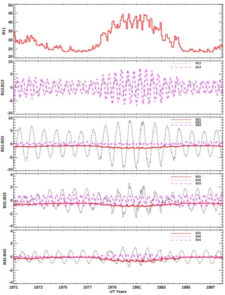
Bn2(d)=(Cn2+Dn2F10.7p(d)+En2Ap(d))cos 2π d 365.25

+ (Fn2+Gn2F10.7p(d)+Hn2Ap(d))sin 2π d 365.25 (5) Bn3(d)=(Cn3+Dn3F10.7p(d)+En3Ap(d))cos

2π d 365.25/2

+ (Fn3+Gn3F10.7p(d)+Hn3Ap(d))sin

2π d 365.25/2 (6) Where n is the n-th EOF coefficient of base func-tion. Bn1(d), Bn2(d), and Bn3(d) correspond to the so-lar cycle, annual, and semi-annual variation components in EOF coefficients respectively, ε is the residual error. F10.7p= (F10.7+ F10.7A)/2, which was established based on

the value of daily F10.7and its 81-day moving average F10.7A.

F10.7p has been used in solar irradiance empirical models as

a solar EUV proxy (e.g., Hinteregger et al., 1973; Richards et al., 1994). It has been validated that F10.7p represents

quite well the intensity of solar EUV flux, which is consid-ered as a better solar proxy for common use (Liu et al., 2006, 2011). Here we use a linear function of F10.7pand Ap to

20 25 30 35 40 45 50

B11

-10 -5 0 5 10

B12,B13

B12 B13

-10 -5 0 5 10

B21-B23

B21 B22 B23

-4 -2 0 2 4

B31-B33

B31 B32 B33

1971 1973 1975 1977 1979 1981 1983 1985 1987

UT Years -4

-2 0 2 4

B41-B43

B41 B42 B43

Fig. 5. Variation components of fitted EOF coefficients with different period.

in EOF coefficients. The amplitudes of those trigonometric functions can also be expressed in the form of linear func-tions of F10.7p and Ap index to show their dependence on

the level of solar activity as well as geomagnetic activity.C, D,E,F,GandHare coefficients of various parts in above equations. Those coefficients can be calculated by using lin-ear regression analysis method, and thus the EOF coefficients An(d)can be acquired by using Eqs. (3)–(6) with those

de-termined coefficients. We can still add shorter periods varia-tion components into the EOF coefficients (e.g., the seasonal variation components, the solar rotational components with the period of 27-days, and 16-days solar oscillation, etc.) for the accuracy of the fitted coefficients. The modeled values of

foF2 at single stations can be acquired using Eq. (2) with the

EOF base functions multiplied by the coefficients calculated with aforementioned linear regression method.

Observed

24

21

18

15

12

9

6

3

0

Local Time (Hour)

Wakkanai

IRI

Wakkanai

EOF

Wakkanai

24

21

18

15

12

9

6

3

0

Local Time (Hour)

Kokubunji Kokubunji Kokubunji

4 6 8 10 12 14 16

1980 Jul 1981 Jul

UT Year 24

21

18

15

12

9

6

3

0

Local Time (Hour)

Yamagawa

1980 Jul 1981 Jul

UT Year

Yamagawa

1980 Jul 1981 Jul 1982

UT Year

Yamagawa

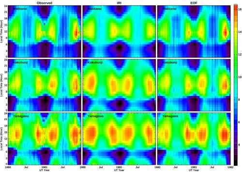
Fig. 6. Comparison among the observational foF2, IRI model value and EOF model value during 1980–1982.

4.3 Data-model comparison and discussion

The model constructed using EOF method combined with linear regression analysis need to be verified via the data-model comparison from which the accuracy of data-model can be evaluated. The data among period of high solar activity years (1980, 1981) and low solar activity years (1986, 1987) are selected from the observational foF2 value as validating samples. One thing worth noting is that the chosen data for data-model comparison is excluded from the original data set when building the model. In other words, the data among the selecting time period is not included in the data set to generate the EOF coefficients, which makes the testing data independent for model validation.

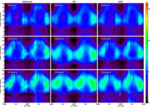
Figures 6 and 7 show the comparison of the daily vari-ation of the observvari-ational foF2 values, the values given by IRI model, and the EOF modeled values during years with high solar activity (1980, 1981) as well as years with low so-lar activity (1986, 1987). It can be seen from the figure that the IRI modeled values have a relatively smooth boundary from which the details of variation in original data set can

not be well expressed. This illustrated that some variation with short periods and small scale irregularities/disturbances are beyond the level that can be well represented by IRI. On the contrary, the EOF modeled values can reflect quite well different scales of variation in original foF2, which is mainly attributed to that the EOF coefficients are directly obtained from the decomposition of original data set. The quick con-vergence of EOF expansion made it possible to use limited number of base functions and the corresponding fitted coef-ficients generated by linear regression analysis to reproduce the observational data set.

Observed

24

21

18

15

12

9

6

3

0

Local Time (Hour)

Wakkanai

IRI

Wakkanai

EOF

Wakkanai

24

21

18

15

12

9

6

3

0

Local Time (Hour)

Kokubunji Kokubunji Kokubunji

0 5 10 15

1986 Jul 1987 Jul

UT Year 24

21

18

15

12

9

6

3

0

Local Time (Hour)

Yamagawa

1986 Jul 1987 Jul

UT Year Yamagawa

1986 Jul 1987 Jul 1988

UT Year Yamagawa

Fig. 7. Comparison among the observational foF2, IRI model value and EOF model value during 1986–1988.

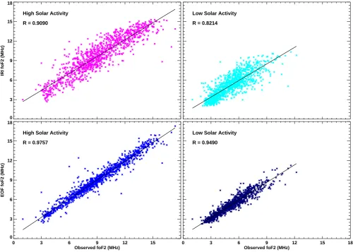
large (e.g., Bilitza et al., 1998, 2006; Bilitza and Williamson, 2000). For EOF model, the cumulative percentage variances of the first 4-order coefficients associated with the principal components of EOF analysis during solar high activity years are higher than that in solar low activity years. No matter for high or low solar activity years, the correlation coefficients between the EOF modeled values and the observational val-ues, which are 0.9757 and 0.9490 respectively, are higher than that for IRI model. So the EOF model can reproduce the original data quite well by better reflecting the temporal distribution characteristics.

As the discrepancies between model and observational values varied with the temporal distribution of foF2, the model-measurements deviation, rather than the model result itself, seems better suited for investigating the accuracy de-gree of the model. Here we use the relative error (RE) and the relative mean square error (RMS) to represent the deviation. The RE and RMS are calculated by the following formulas.

RE= 1

N

N

X

i=1

_foF2

model−foF2obs

foF2obs

×100 % (7)

RMS= v u u t 1 N

N

X

i=1

_foF2

model−foF2obs

foF2obs

2

×100 % (8)

0 3 6 9 12 15 18

IRI foF2 (MHz)

High Solar Activity

R = 0.9090

Low Solar Activity

R = 0.8214

0 3 6 9 12 15

Observed foF2 (MHz) 0

3 6 9 12 15 18

EOF foF2 (MHz)

High Solar Activity

R = 0.9757

0 3 6 9 12 15 18

Observed foF2 (MHz) Low Solar Activity

R = 0.9490

Fig. 8. Scatter plots of IRI and EOF model values versus observational data of foF2.

the accumulated percentages of first 4-order coefficients of EOF base function.

Figure 10 shows the long-term variation of relative errors and relative mean square errors between the model and the observational data in day (6 a.m.–6 p.m.) and night (6 p.m.– 6 a.m.). The IRI model results are obviously inferior to that of EOF model results, and there are some other features worth noting. First, there are distinct semi-annual variation components in the relative errors of EOF model. Second, the wave crest and the wave trough of the variation of relative er-rors are asymmetric for day and night. In the daytime, the rel-ative errors have positive values (near wave crest) or increas-ing trends around solstice and the negative values (near wave trough) or decreasing trends around equinox. However, the night time conditions are to the contrary. Positive error ap-pears near equinox and negative error apap-pears near solstice. For the seasonal asymmetry, three different explanations are suggested: (1) neutral wind hypothesis: the large-scale in-terhemispheric circulation induced by asymmetric heat dis-tribution can cause asymmetric density variation (Johnson and Gottlieb, 1970; Fuller-Rowell, 1998). The circulation

may also exert influence on foF2 and even on deviation with small scales due to the proportional relation between foF2 and electron density. (2) Equinoctial hypothesis: the vari-ation of ionospheric parameters are related to the angle be-tween solar wind flow and geomagnetic dipole field and to the solar asymmetric illumination (McIntosh, 1959; Lyatsky et al., 2001). (3) Axial hypothesis: the increase of helio-graphic latitude around equinoxes can place Earth closer to fast solar wind streams from coronal holes (Bohlin, 1977).

5 Summary and conclusions

low solar activity

-20 -10 0 10 20 30 40

IRI Dif (%)

Spring (RMS: 4.74%)

(RMS: 7.43%)

high solar activity

-6 -4 -2 0 2 4 6

EOF Dif (%)

Spring _{(RMS: 1.13%)}

(RMS: 1.19%)

-20 -10 0 10 20 30 40

IRI Dif (%)

Summer (RMS: 11.95%)

(RMS: 7.20%)

-6 -4 -2 0 2 4 6

EOF Dif (%)

Summer _{(RMS: 0.83%)}

(RMS: 2.69%)

-20 -10 0 10 20 30 40

IRI Dif (%)

Autumn _{(RMS: 6.22%)}

(RMS: 8.09%)

-6 -4 -2 0 2 4 6

EOF Dif (%)

Autumn _{(RMS: 1.38%)}

(RMS: 1.67%)

0 4 8 12 16 20 24

Local Time (Hours) -20

-10 0 10 20 30 40

IRI Dif (%)

Winter (RMS: 15.00%)

(RMS: 10.39%)

0 4 8 12 16 20 24

Local Time (Hours) -6

-4 -2 0 2 4 6

EOF Dif (%)

Winter _{(RMS: 2.13%)}

(RMS: 1.81%)

Fig. 9. Diurnal variation of relative errors and relative mean square errors between model and the observational data.

First, ionospheric foF2 is subject to a number of drivers which can be broadly divided into three categories: solar ion-izing radiation, geomagnetic activity and meteorological in-fluences. It is feasible to use F10.7, X-ray fluxes, solar zenith

angle and Ap index as appropriate proxies to reflect the afore-mentioned influences and to refill the missing value of origi-nal foF2 with similar-parameters method.

Second, the EOF model can reproduce quite well the orig-inal data sets of foF2 by utilizing only the first 4-order base

functions as well as corresponding coefficients. The base functions can express the diurnal variation of the original

foF2 data while the corresponding coefficients can represent

the long-term variation (solar cycle, annual, semi-annual, seasonal, solar rotation, and irregularities, etc.).

-10 -5 0 5 10 15 20 25 30

Difference (%)

IRI model (RMS: 10.14%) EOF model (RMS: 0.93%) Day

-10 -5 0 5 10 15 20 25 30

Difference (%)

IRI model (RMS: 8.54%) EOF model (RMS: 0.88%) Day

1980 Apr Jul Oct 1981 Apr Jul Oct 1982 Universal Time

-10 -5 0 5 10 15 20 25 30

Difference (%)

IRI model (RMS: 9.68%) EOF model (RMS: 0.70%) Night

1986 Apr Jul Oct 1987 Apr Jul Oct 1988 Universal Time

-20 -15 -10 -5 0 5 10 15 20

Difference (%)

IRI model (RMS: 7.31%) EOF model (RMS: 1.11%) Night

Fig. 10. Long-term variation of relative errors and relative mean square errors between model and the observatioanl data.

can reflect the major change tendencies and the temporal dis-tribution characteristics of the mid-latitude ionosphere of the Sea of Japan region.

Finally, the error analysis reveals that there are seasonal anomaly and semi-annual variation phenomena. These re-sults can be attributed to neutral wind hypothesis, equinoctial hypothesis, and axial hypothesis.

Acknowledgements. This research was jointly supported by the

National Natural Science Foundation of China (41174134 and 40904036), National Important basic Research Project of China (2011CB811405), the State Key Laboratory of Space Weather, and the China Scholarship Council (2009601221). The F10.7 index data, Geomagnetic Ap index data and ionospheric foF2 data for Wakkanai, Kokubunji and Yamagawa were downloaded from the SPIDR (Space Physics Interactive Data Resource) website: http: //spidr.ngdc.noaa.gov/spidr/home.do.

Topical Editor K. Kauristie thanks two anonymous referees for their help in evaluating this paper.

References

Adeniyi, J. O., Bilitza, D., Radicella, S. M., and Willoughby, A. A.: Equatorial F2-peak parameters in the IRI model, Adv. Space Res., 31, 507–512, doi:10.1016/S0273-1177(03)00039-5, 2003. Bilitza, D.: International Reference Ionosphere 2000, Radio Sci.,

36, 261–275, doi:10.1029/2000rs002432, 2001.

Bilitza, D. and Reinisch, B. W.: International Reference Ionosphere 2007: Improvements and new parameters, Adv. Space Res., 42, 599–609, doi:10.1016/j.asr.2007.07.048, 2008.

Bilitza, D. and Williamson, R.: Towards a better representation of the IRI topside based on ISIS and Alouette data, Adv. Space Res., 25, 149–152, doi:10.1016/S0273-1177(99)00912-6, 2000. Bilitza, D., Rawer, K., Bossy, L., Kutiev, I., Oyama, K., Leitinger,

R., and Kazimirovsky, E.: International Reference ionosphere 1990, Nat. Space Sci. Data Cent., Report 90-22, Greenbelt, Md., 1990.

Bilitza, D., Koblinsky, C., Williamson, R., and Bhardwaj, S.: Im-proving the topside electron density model for IRI, Adv. Space Res., 22, 777–787, doi:10.1016/S0273-1177(98)00098-2, 1998. Bilitza, D., Reinisch, B. W., Radicella, S. M., Pulinets,

S., Gulyaeva, T., and Triskova, L.: Improvements of the International Reference Ionosphere model for the top-side electron density profile, Radio Sci., 41, RS5S15, doi:10.1029/2005RS003370, 2006.

Bohlin, J. D.: Extreme-ultraviolet observations of coronal holes., Sol. Phys., 51, 377–398, doi:10.1007/BF00216373, 1977. CCIR: Comite Consultatif International des Radiocommunications,

Reports 340, 340-2 and later supplements, Geneva, 1967. Daniell, R. E., Brown, L. D., Anderson, D. N., Fox, M. W., Doherty,

P. H., Decker, D. T., Sojka, J. J., and Schunk, R. W.: Parame-terized ionospheric model: A global ionospheric parameteriza-tion based on first principles models, Radio Sci., 30, 1499–1510, doi:10.1029/95RS01826, 1995.

Forbes, J. M., Palo, S. E., and Zhang, X.: Variability of the ionosphere, J. Atmos. Sol. Terr. Phys., 62, 685–693, doi:10.1016/S1364-6826(00)00029-8, 2000.

Fuller-Rowell, T. J.: The “thermospheric spoon”: A mechanism for the semiannual density variation, J. Geophys. Res., 103, 3951– 3956, doi:10.1029/97JA03335, 1998.

Hinteregger, H. E., Bedo, D. E., and Manson, J. E.: The EUV spec-troheliometer on Atmosphere Explorer., Radio Sci., 8, 349–359, doi:10.1029/RS008i004p00349, 1973.

Johnson, F. S. and Gottlieb, B.: Eddy mixing and circula-tion at ionospheric levels, Planet. Space Sci., 18, 1707–1718, doi:10.1016/0032-0633(70)90004-8, 1970.

Kumluca, A., Tulunay, E., Topalli, I., and Tulunay, Y.: Tem-poral and spatial forecasting of ionospheric critical fre-quency using neural networks, Radio Sci., 34, 1497–1506, doi:10.1029/1999RS900070, 1999.

Lei, J., Burns, A. G., Tsugawa, T., Wang, W., Solomon, S. C., and Wiltberger, M.: Observations and simulations of quasiperiodic ionospheric oscillations and large-scale traveling ionospheric disturbances during the December 2006 geomagnetic storm, J. Geophys. Res., 113, A06310, doi:10.1029/2008JA013090, 2008a.

Lei, J., Thayer, J. P., Forbes, J. M., Wu, Q., She, C., Wan, W., and Wang, W.: Ionosphere response to solar wind high-speed streams, Geophys. Res. Lett., 35, L19105, doi:10.1029/2008GL035208, 2008b.

Liang, S.: The Deviation of IRI from the Ionospheric Parameters Observed Over East Asia, Publications of the Yunnan Observa-tory, 128, 1–+, 1990.

Liu, C., Zhang, M., Wan, W., Liu, L., and Ning, B.: Model-ing M(3000)F2 based on empirical orthogonal function analysis method, Radio Sci., 43, RS1003, doi:10.1029/2007RS003694, 2008.

Liu, L., Wan, W., and Ning, B.: Statistical modeling of ionospheric foF2 over Wuhan, Radio Sci., 39, RS2013, doi:10.1029/2003RS003005, 2004.

Liu, L., Wan, W., Ning, B., Pirog, O. M., and Kurkin, V. I.: So-lar activity variations of the ionospheric peak electron density, J. Geophys. Res., 111, A08304, doi:10.1029/2006JA011598, 2006. Liu, L., Wan, W., and Le, H.: Solar activity effects of the iono-sphere: A brief review, Chinese Science Bulletin, 56, 1202– 1211, doi:10.1007/s11434-010-4226-9, 2011.

Lyatsky, W., Newell, P. T., and Hamza, A.: Solar illu-mination as cause of the equinoctial preference for ge-omagnetic activity, Geophys. Res. Lett., 28, 2353–2356, doi:10.1029/2000GL012803, 2001.

Mao, T., Wan, W., Yue, X., Sun, L., Zhao, B., and Guo, J.: An em-pirical orthogonal function model of total electron content over China, Radio Sci., 43, RS2009, doi:10.1029/2007RS003629, 2008.

Marsh, D. R., Solomon, S. C., and Reynolds, A. E.: Empirical model of nitric oxide in the lower thermosphere, J. Geophys. Res., 109, A07301, doi:10.1029/2003JA010199, 2004.

Matsuo, T. and Forbes, J. M.: Principal modes of thermospheric density variability: Empirical orthogonal function analysis of CHAMP 2001-2008 data, J. Geophys. Res., 115, A07309, doi:10.1029/2009JA015109, 2010.

Matsuo, T., Richmond, A. D., and Nychka, D. W.: Modes of high-latitude electric field variability derived from DE-2

mea-surements: Empirical Orthogonal Function (EOF) analysis, Geo-phys. Res. Lett., 29, 1107, doi:10.1029/2001GL014077, 2002. Matsuo, T., Richmond, A. D., and Lu, G.: Optimal interpolation

analysis of high-latitude ionospheric electrodynamics using em-pirical orthogonal functions: Estimation of dominant modes of variability and temporal scales of large-scale electric fields, J. Geophys. Res., 110, A06301, doi:10.1029/2004JA010531, 2005. McIntosh, D. H.: On the Annual Variation of Magnetic Distur-bance, Philos. Trans. R. Soc. London. Ser. A., 251, 525–552, doi:10.1098/rsta.1959.0010, 1959.

McKinnell, L. and Oyeyemi, E.: Progress towards a new global foF2 model for the International Reference Ionosphere (IRI), Adv. Space Res., 43, 1770–1775, doi:10.1016/j.asr.2008.09.035, 2009.

McKinnell, L. and Oyeyemi, E.: Equatorial predictions from a new neural network based global foF2 model, Adv. Space Res., 46, 1016–1023, doi:10.1016/j.asr.2010.06.003, 2010.

Mendillo, M., Rishbeth, H., Roble, R., Damboise, E., and Wro-ton, J.: Ionospheric variability originating from tropospheric and stratospheric sources, EOS, 79, 238, 1998.

Mikhailov, A. V., Depuev, V. H., and Depueva, A. H.: Synchronous

NmF2 and NmE daytime variations as a key to the mechanism of

quiet-time F2-layer disturbances, Ann. Geophys., 25, 483–493, doi:10.5194/angeo-25-483-2007, 2007.

Mikhailov, A. V., Depueva, A. H., and Depuev, V. H.: Quiet time F2-layer disturbances: seasonal variations of the occur-rence in the daytime sector, Ann. Geophys., 27, 329–337, doi:10.5194/angeo-27-329-2009, 2009.

Oyeyemi, E. O., Poole, A. W. V., and McKinnell, L. A.: On the global model for foF2 using neural networks, Radio Sci., 40, RS6011, doi:10.1029/2004RS003223, 2005.

Oyeyemi, E. O., McKinnell, L., and Poole, A.: Near-real time foF2 predictions using neural networks, J. Atmos. Sol. Terr. Phys., 68, 1807–1818, doi:10.1016/j.jastp.2006.07.002, 2006.

Pearson, K.: On Lines and Planes of Closest Fit to Systems of Points in Space, Philosophical Magazine, 2, 559–572, 1901. Petrukovich, A. A. and Zakharov, M. Y.:ap-index solar wind

driv-ing function and its semiannual variations, Ann. Geophys., 25, 1465–1469, doi:10.5194/angeo-25-1465-2007, 2007.

Richards, P. G., Fennelly, J. A., and Torr, D. G.: EUVAC: a solar EUV flux model for aeronomic calculations., J. Geophys. Res., 99(A5), 8981–8992, doi:10.1029/94JA00518, 1994.

Rishbeth, H. and Mendillo, M.: Patterns of F2-layer variability, J. Atmos. Sol. Terr. Phys., 63, 1661–1680, doi:10.1016/S1364-6826(01)00036-0, 2001.

Roble, R. G. and Ridley, E. C.: A thermosphere-ionosphere-mesosphere-electrodynamics general circulation model (time-GCM): Equinox solar cycle minimum simulations (30–500 km), Geophys. Res. Lett., 21, 417–420, doi:10.1029/93GL03391, 1994.

Rush, C. M.: URSI foF2 model maps (1988), Planet. Space Sci., 40, 546–547, doi:10.1016/0032-0633(92)90181-M, 1992. Schunk, R. and Nagy, A. (Eds.): Ionospheres: Physics, Plasma

Physics and Chemistry, Cambridge University Press, 2000. Singer, W. and Dvinskikh, N. I.: Comparison of empirical models

of ionospheric characteristics developed by means of different mapping methods, Adv. Space Res., 11, 3–6, doi:10.1016/0273-1177(91)90311-7, 1991.

C. R., De Zeeuw, D. L., Hansen, K. C., Kane, K. J., Manchester, W. B., Oehmke, R. C., Powell, K. G., Ridley, A. J., Roussev, I. I., Stout, Q. F., Volberg, O., Wolf, R. A., Sazykin, S., Chan, A., Yu, B., and K´ota, J.: Space Weather Modeling Framework: A new tool for the space science community, J. Geophys. Res., 110, A12226, doi:10.1029/2005JA011126, 2005.

Vlasov, M. N. and Kelley, M. C.: Crucial discrepancy in the bal-ance between extreme ultraviolet solar radiation and ion densities given by the international reference ionosphere model, J. Geo-phys. Res., 115, A08317, doi:10.1029/2009JA015103, 2010. Xu, W. and Kamide, Y.: Decomposition of daily geomagnetic

vari-ations by using method of natural orthogonal component, J. Geo-phys. Res., 109, A05218, doi:10.1029/2003JA010216, 2004. Xu, Z., Wu, J., Igarashi, K., Kato, H., and Wu, Z.: Long-term

ionospheric trends based on ground-based ionosonde observa-tions at Kokubunji, Japan, J. Geophys. Res., 109, A09307, doi:10.1029/2004JA010572, 2004.

Zapfe, B., Materassi, M., Mitchell, C., and Spalla, P.: Imaging of the equatorial ionospheric anomaly over South America–A sim-ulation study of total electron content, J. Atmos. Sol. Terr. Phys., 68, 1819–1833, doi:10.1016/j.jastp.2006.05.025, 2006.

Zhang, D. H., Mo, X. H., Cai, L., Zhang, W., Feng, M., Hao, Y. Q., and Xiao, Z.: Impact factor for the ionospheric total electron content response to solar flare irradiation, J. Geophys. Res., 116, A04311, doi:10.1029/2010JA016089, 2011.

Zhang, M. L., Shi, J. K., Wang, X., Wu, S. Z., and Zhang, S. R.: Comparative study of ionospheric characteristic pa-rameters obtained by DPS-4 digisonde with IRI2000 for low latitude station in China, Adv. Space Res., 33, 869–873, doi:10.1016/j.asr.2003.07.013, 2004.

Zhang, M., Shi, J., Wang, X., Shang, S., and Wu, S.: Ionospheric behavior of the F2 peak parameters foF2 and hmF2 at Hainan and comparisons with IRI model predictions, Adv. Space Res., 39, 661–667, doi:10.1016/j.asr.2006.03.047, 2007.

Zhang, M.-L., Liu, C., Wan, W., Liu, L., and Ning, B.: A global model of the ionospheric F2 peak height based on EOF anal-ysis, Ann. Geophys., 27, 3203–3212, doi:10.5194/angeo-27-3203-2009, 2009.