Reconstruction of Hydrometric Data Using a Network Optimization Model

Reconstruction of Hydrometric Data Using a

Network Optimization Model

Ayoub TAHIRI

_{, David LADEVEZE}

_{, Pascale CHIRON}

_{, Bernard}

ARCHIMEDE

1 _{CACG, BP 449, Chemin de Lalette, 65000 Tarbes Cedex, France}

2 _{Laboratoire Génie de Production, LGP, Université de Toulouse, INP-ENIT, Tarbes, France.}

[email protected], [email protected], [email protected], [email protected]

Abstract

Water resource managers need to implement precise and efficient water management methods particularly in the context of low flow water management. The management objectives are complex because managers must satisfy both water demands for human activities and environmental goals. More often the flow objectives are defined at specific strategic points in which hydrometric stations are based. In order to allow the manager to better understand the hydrographical network behavior, in particular for inter-basin water transfer, these strategic hydrometric stations must be reinforced by some intermediate hydrometric stations, by modeling the network behavior, and by introducing weather forecast data in order to simulate the evolution in time and space of the river. For an efficient management, it is essential that the data collected and the output of the models (the natural flow and the withdrawals) must be reliable. For this purpose, a network optimization model was developed for analyzing the consistency of the available data set (measurements and model outputs) on a hydraulic system. Herein, a reconstruction of hydrometric data using this network optimization model is applied to the Arrats watershed management.

1

Introduction

The management of water resources within a catchment area during low water periods aims to ensure the environmental needs and to satisfy the needs for consumer and economic uses. It is based on a good knowledge of the river hydraulicity and on an estimation of its evolution in time. The hydrometric measurement is an integrating indicator for almost all the factors that govern the water cycle at the level of a watershed. The monitoring of the objective flows associated with the reference measurement stations allows only a simple understanding of the system state. In the case of

* _{Masterminded EasyChair, and created the first draft and the first stable version of this document}

Engineering

Volume 3, 2018, Pages 139–146

basin water transfer, these reference hydrometric stations must be reinforced by additional hydrometric stations producing intermediate states and allowing to control the release of water for low water replenishment complying with the flow travel time. The position of the measuring stations follows several geographical and hydrological principles. In general, a transfer time of one day separate two measuring stations (i.e. approximately every 40 km). Additional measuring stations may be located at confluences, to cover the entire basin and increase the number of information needed for management. The distribution of the withdrawal points along the river and the hydrology of each basin define as well the location of the measurement stations.

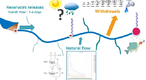
Considering a refilled watershed, the main rivers of the network are replenished during the low-water-periods thanks to the previous water storage in reservoirs (Figure 1). In order to achieve the predefined flow objectives, the water resource manager needs to adapt the water flow released from the reservoirs and the inter-basin water transfer volumes in canal to satisfy the objective flows (integrating the needs for the environment), while satisfying all uses (irrigation, drinking water, industries, tourism, fishing ...).

Figure 1: Diagram of the different parameters influencing the watershed management.

The water time delay between the reservoir and the downstream point is usually one or two days (sometimes 4 days). Hence, the flow evolution depending on the weather, the inflows and the withdrawals need to be forecasted through the use of models and data measured in intermediate hydrometric stations. Forecasts of flows and withdrawals are estimated by hydrological approaches (for natural flows) and environmental considerations (for agricultural withdrawals). Hence, for an efficient management, it is essential that the data collected and the outputs of the models (the natural flow and the withdrawals) must be reliable. For this purpose, a network optimization model was developed for analyzing the consistency of the available data set (measurements and model outputs) on a hydraulic system. This method allows to:

 assess and improve the measurements (noisy data, missing data, aberrant data) through the use of data consistency analysis.

 simulate non-acquired physical parameters (local inflows, draw-off, river longitudinal section discharge value).

It consists to find the optimal consistent flow fitting the values of the output model variables and the acquired data with respect to the values of the confidence criteria for measurement (flow, volume) and of the other available information (draw-off, rain, temperature…)

time step (hourly, daily ...) over a computation horizon formulated in number of periods. Fixed transfer times, expressed as whole numbers of periods, are also taken into account.

2

The network optimization model

2.1

Framework

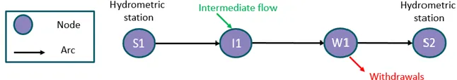
The hydraulic system is modeled with a network flow model (Bertsekas, 1998). A network flow model 𝒢 = (𝒱, 𝒜) is a direct graph which consists in a set 𝒱 of nodes and a set 𝒜 of arcs connecting pair of nodes. The nodes stand for either a hydrometric station (denoted Si) or an intake point

(denoted Wi) or a local inflow point (denoted Ii) as illustrated in the example given in Figure 2. The

quantity of water flow crossing each arc is designed as the flow of an arc, and for each node N in 𝒱, the conservation of the flow law must be satisfied i.e. the sum of the flows outgoing from a node N is equal to the sum of the flows incoming it.

Figure 2: A network model of a reach.

In the example described in Figure 2, the reach is composed of one intake point, one confluence (inflow point) and two hydrometric stations on its extremities. The conservation of flows balance can be written as:

𝑄2(t) + ∆𝑄2(t) = (𝑄1(t − 𝑇𝑆1→𝑆2) + ∆𝑄1(𝑡 − 𝑇𝑆1→𝑆2)) + (𝐼𝐹(t − 𝑇𝐼1→𝑆2) + ∆𝐼𝐹(𝑡 −

𝑇𝐼1→𝑆2))−(𝑊𝐼(t − 𝑇𝑊1→𝑆2) + ∆WI(t − 𝑇𝑊1→𝑆2)) (1)

where 𝑡 is the time, 𝑇𝑖→𝑗 is the transfer time delay between the node 𝑖 and the node 𝑗, 𝑄1 is the

flow outgoing the node 𝑆1, 𝑄2 is the flow incoming the node 𝑆2, 𝐼𝐹 is the flow incoming the node 𝐼1,

𝑊𝐼 is the flow outgoing the node 𝑊1, and ∆∅ is the potential error for a flow ∅. The unknowns of the

equation are ∆∅, and are not static in time.

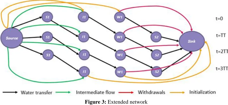
In order to include the transfer time delays in the network flow, the time expanded network formalism proposed by Fulkerson (Fulkerson, 1966) is applied: the nodes are duplicated at each time step over the duration of the simulation, and the transit times and flow are implicit in arcs linking those copies.

Figure 3 represents the extended network corresponding to the reach presented in Figure 2. To simplify the example, we considered a constant time transfer between the nodes. The extended network in the example covers a period of 3TT (Time Transfer).

In order to obtain a single source network, we consider two additional nodes: source and sink nodes.

Figure 3: Extended network

The colors of the arcs, and the nature of the nodes are only used for representation reasons and are not used in the execution of the optimization algorithm.

2.2

The optimal consistent flow

The hydraulic system is modeled with a network flow model (Bertsekas, 1998). A network flow model 𝒢 = (𝒱, 𝒜) is a direct graph which consists in a set 𝒱 of nodes and a set 𝒜 of arcs connecting pair of nodes. The nodes stand for either a hydrometric station (denoted Si) or an intake point

(denoted Wi) or a local inflow point (denoted Ii) as illustrated in the example given in Figure 2. The

quantity of water flow crossing each arc is designed as the flow of an arc, and for each node N in 𝒱, the conservation of the flow law must be satisfied i.e. the sum of the flows outgoing from a node N is equal to the sum of the flows incoming it.

Equation (1), corresponding to the conservation of flows balance can be written as:

(𝑄2(𝑡)− 𝑊𝐼(𝑡 − 𝑇𝑊→𝑆2)) − (𝑄1(𝑡 − 𝑇𝑆1→𝑆2) + 𝐼𝐹(𝑡 − 𝑇𝐼→𝑆2)) = (∆𝑄1(𝑡 − 𝑇𝑆1→𝑆2) + ∆𝐼𝐹(𝑡 −

𝑇𝐼→𝑆2)) − (∆ 𝑊𝐼(𝑡 − 𝑇𝑊→𝑆2) +∆𝑄2(𝑡)) (2)

If the measurements and the outputs of the models were perfect, the first term of the equation (2) would be equal to zero: (𝑄2(t)− 𝑊𝐼(t − 𝑇𝑊→𝑆2)) − (𝑄1(t − 𝑇𝑆1→𝑆2) + 𝐼𝐹(t − 𝑇𝐼→𝑆2)) = 0

Finding the consistent flow consists in distributing the error which corresponds to the difference between the flow releasing the source node and the flow absorbed by the sink node.

The optimal consistent flow is obtained by minimizing the weighted sum of the errors (i.e. ∆∅ in equation (1)) (Goldberg & Tarjan, 1989) associated with each information, assuming that the weights are a function of precision and tolerance criteria, transcribed in the graph in the form of cost functions associated to the arcs. The reconstruction of the flows consists in calculating a consistent flow of minimal cost. The cost of the graph is the sum of the costs of all the arcs of the graph.

The hydraulic discharges are recovered from computing the minimum cost flow on the graph. The minimum cost flow problem is given by:

𝑚𝑖𝑛 ∑𝑖∈𝒜𝑐𝑜𝑠𝑡(∆𝜙𝑖) (3)

subject to the Kirchhoff constraints on every node except the source and the sink nodes, and where

𝑐𝑜𝑠𝑡(∆𝜙𝑖) is the cost of the flow carried by the arc 𝑖. The available flow to be distributed over the

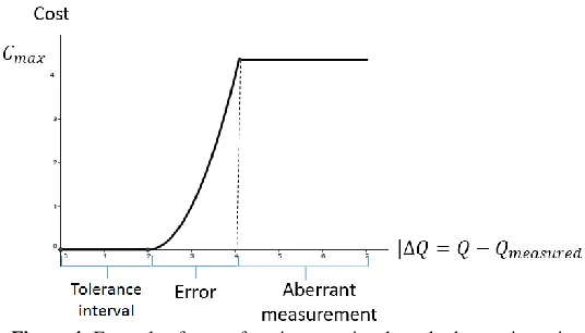
The definition of cost functions is mainly based on the water manager experience. For hydrometric stations the essential parameter is the stream gauging quality. A tolerance interval is assigned to each variable. It is defined as a constant for each station and each model output.

Figure 4: Example of a cost function associated to a hydrometric station

Inasmuch as the in-situ measurements are supposed more accurate than data computed from the withdrawal and natural input models, the tolerance interval for the stations variables are sharper. Inside the confidence interval, the cost is null, great beyond the cost function is quadratic and convex (see Figure 4). The convexity of the cost functions enables the distribution of the errors over the system. Finally, after the optimum flow computation, if an arc cost has a value greater than a predefined maximum value (Cmax ), the data is marked as an outlier and is discarded.

2.3

The optimal algorithm

The hydraulic system is modeled with a network flow model (Bertsekas, 1998). A network flow model 𝒢 = (𝒱, 𝒜) is a direct graph which consists in a set 𝒱 of nodes and a set 𝒜 of arcs connecting pair of nodes. The nodes stand for either a hydrometric station (denoted Si) or an intake point

(denoted Wi) or a local inflow point (denoted Ii) as illustrated in the example given in Figure 2. The

quantity of water flow crossing each arc is designed as the flow of an arc, and for each node N in 𝒱, the conservation of the flow law must be satisfied i.e. the sum of the flows outgoing from a node N is equal to the sum of the flows incoming it.

The graph 𝒢 is associated to a residual graph 𝒢′ _{(Evans, 1992) composed of forward arcs and}

backward arcs. The concept of the method developed herein for looking for optimality extends the work developed by Klein (Klein, 1967) for constant positive unit costs over arcs. The basic scheme is described by the algorithm 1.

cycle implies that the current flow can be improved by moving a portion of the flow through the cycle. Canceling a cycle with a large negative cost and with a large residual capacity would significantly improve the objective function.

Many algorithms exist to find negative cost cycles in a directed graph, such as: Bellman–Ford algorithm (Bellman, 1958), Floyd-Warshall algorithm (Floyd, 1962), A* algorithm (Hart, Nilsson, & Raphael, 1968). Herein, the Bellman-Ford algorithm is implemented since it was observed that it is the most efficient for our situation.

To cancel a negative cost cycle, a computed amount of the flow, 𝛿∅, is displaced around the cycle to obtain a zero-cost cycle, or to saturate an arc of the cycle. A cycle is an independent subgraph of the graph 𝒢, hence improving the cost of a cycle would improve the cost of the network. The optimum flow 𝛿∅ which should be displaced on a negative cycle in order to optimize its cost is given by:

𝛿∅ = −𝜎

𝜃 (4)

where 𝜎 is the cost of the cycle and 𝜃 is the sum of the first derivatives of the cost functions of the arcs belonging to the cycle (Tahiri, Ladeveze, Chiron, Archimède, & Lhuissier, 2018)].

3

The Arrats watershed management case

The graph modelling and data reconstruction method were applied on the Arrats watershed. The Arrats river is an affluent of the Garonne river the flow of which depends on the water stored in the Astarac lake (10Mm3) and on upstream inflows incoming from the Neste channel.

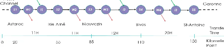
The river is equipped with five hydrometric stations: Astarac (S1), Isle Arné (S2), Mauvezin (S3), Bives (S4), and St-Antoine (S5). Since the points of withdrawals on the river are numerous, we consider a representative withdrawal point at the center of each reach (W1, W2, W3, W4). The natural inflows join the river at the outlet of the three intermediate watersheds (Isle Arné, Bives and St-Antoine) (see Figure 5).

Figure 5: The Arrats watershed model.

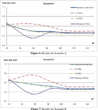
In the scenario A, the reconstructed flows are close to the measured values except for the Isle Arné station. According to the water managers, this station is not a reliable station, which is confirmed: the flows are underestimated. Thus, thanks to the data reconstruction method proposed herein, the outlier values can be adjusted. In the case of the four others stations, the reconstructed flows are magnitude consistent with measured flows. However, the confidence interval values highlight the weak measurement accuracy. At the level of the excluded stations Isle Arné and Mauvezin, the confidence interval is larger in the B case than in the A case. Thus, in the B case even if the discharges are estimated thanks to the model, the accuracy is weaker than when the measurement is done. Therefore, these two hydrometric stations are essential for flow reconstruction, although the Isle Arné station is quite unreliable.

Figure 6: Results for Scenario A

Figure 7: Results for Scenario B

From these results, it can be estimated that if the water manager establishes his decisions according to the Isle Arné station, a loss of 300 to 600.000 𝑚3 _{per year will occur. This demonstrates}

that the flow reconstruction algorithm can reduce the risks taken by the manager.

This experimentation leads to the conclusion that the model is robust to the aberrant data of Isle Arné station, and that establishing a new hydrometric station network at the upstream will lead to a better management.

4

Conclusion

The graph modelling and the optimal consistent flow optimization produces meaningful additional information to the acquired data, and allows to:

 discriminate the aberrant data due to either outliers or to ungauged/unreliable stations,

 replace the imprecise values with reconstructed data associated to a well-known reliability interval,

 assist the water manager to locate the additional hydrometric stations (maintain or remove the existing stations, add new station),

Water managers are thinking more and more about how they can optimize the number of hydrometric stations on a network, mainly due to economic reasons. For example, in the 1980s and 1990s, considerable reductions in the density of hydrological networks have been found in many countries: Canada (-21%), Finland (-7%), New Zealand (-20%) and the United States (-6%) (World Meteorological Organization, 2008). Hence, the algorithm proposed in this paper may replace the lack of hydrometric stations.

In this work, volumes were considered to be carried as solids, which means that their deformation weren’t considered. Future work will focus on the integration of the hydraulic constraints in the model and particularly the water transfer deformation.

References

Bellman, R. (1958). On a routing problem. Quarterly of applied mathematics, 16, 87-90.

Bertsekas, P. D. (1998). Network optimization: continuous and discrete models. Belmont, Massachusetts: Athena Scientific.

Evans, J. (1992). Optimization algorithms for networks and graphs. CRC Press. Floyd, R. W. (1962). Algorithm 97: shortest path. Communications of the ACM, 5, 345.

Fulkerson, D. R. (1966). Flow networks and combinatorial operations research. The American Mathematical Monthly, 73, 115-138.

Goldberg, A. V., & Tarjan, R. E. (1989). Finding minimum-cost circulations by canceling negative cycles. Journal of the ACM, 36, 873-886.

Hart, P. E., Nilsson, N. J., & Raphael, B. (1968). A formal basis for the heuristic determination of minimum cost paths. IEEE transactions on Systems Science and Cybernetics, 4, 100-107. Klein, M. (1967). A primal method for minimal cost flows with applications to the assignment and

transportation problems. Management Science, 14, 205-220.

Saaty, T. L., & Busacker, R. G. (1965). Finite Graphs and Networks: an introduction with applications. McGraw-Hill Book Company.

Tahiri, A., Ladeveze, D., Chiron, P., Archimède, B., & Lhuissier, L. (2018). Reservoir Management Using a Network Flow Optimization Model Considering Quadratic Convex Cost Functions on Arcs. Water Resources Management, 1-14.

Tanguy, J. M. (2010). Environmental Hydraulics: Mathematical Models. John Wiley & Sons.