R E S E A R C H A R T I C L E
Open Access
A multi-arm multi-stage clinical trial design for
binary outcomes with application to
tuberculosis
Daniel J Bratton
*, Patrick PJ Phillips and Mahesh KB Parmar
Abstract
Background: Randomised controlled trials are becoming increasingly costly and time-consuming. In 2011, Royston and colleagues proposed a particular class of multi-arm multi-stage (MAMS) designs intended to speed up the evaluation of new treatments in phase II and III clinical trials. Their design, which controls the type I error rate and power for each pairwise comparison, discontinues randomisation to poorly performing arms at interim analyses if they fail to show a pre-specified level of benefit over the control arm. Arms in which randomisation is continued to the final stage of the trial are compared against the control on a definitive time-to-event outcome measure. To increase efficiency, interim comparisons can be made on an intermediate time-to-event outcome which is on the causal pathway to the definitive outcome.
Methods: We adapt Royston’s MAMS design to binary outcomes observed at the end of a fixed follow-up period and analysed using an absolute difference in proportions. We apply the design to tuberculosis (TB), an area where many new drugs are in development, and demonstrate how it can greatly accelerate the evaluation of new TB regimens. We use simulations to support the extensions to the methodology and to investigate the amount of bias in the estimated treatment effects of arms in which randomisation is ceased at the first interim analysis and arms which continue to the final stage of the trial.
Results: The proposed seamless phase II/III TB trial designs are shown to greatly reduce sample size requirements and trial duration compared to conducting separate phase II and III trials. The bias in the estimated treatment effects for the definitive outcome is shown to be small, especially when treatment selection is based on an intermediate outcome or when a reanalysis is performed at the planned end of the trial after all recruited patients have completed follow-up.
Conclusions: The proposed designs are practical and could be used in a variety of disease areas. They hold
considerable promise for speeding up the evaluation of new treatments particularly in TB where many new regimens will soon be available for testing in phase II and phase III trials.
Keywords: Multi-arm, Multi-stage, Tuberculosis, Binary outcome, Adaptive design, Treatment selection
Background
In recent years the pace of drug development in some disease areas has rapidly increased. Despite this, there has been a slowdown in the rate of new therapies reach-ing patients [1]. This is largely due to the increasreach-ing cost and inefficiency of the drug development process and that most new treatments have no clear benefit over standard care. As a result, the US Food and Drug Administration
*Correspondence: [email protected]
Medical Research Council Clinical Trials Unit at University College London, 125 Kingsway, London, UK
(FDA) has called for a new ‘product development toolkit’ for improving the predictability and efficiency of clinical trials.
Due to the acceleration in drug development it is now more common for multiple new treatments to be simul-taneously available for testing in clinical trials. In tuber-culosis (TB), for example, there are currently at least ten new or repurposed drugs in the clinical pipeline [2-4]. Since TB is treated using a combination of drugs rather than monotherapy, the number of regimens that could potentially be assessed in phase II or III trials
in the near future is vast. Evaluating each new treat-ment against a control in separate two-arm trials will not only require a huge amount of resources but may deny patients access to the most effective, simplest and shortest new regimens as early as possible. Innovative trial designs which are able to efficiently assess multi-ple new treatments simultaneously are therefore urgently needed.
In discussing such an issue, Phillips et al. [5] have sug-gested the use of the multi-arm multi-stage (MAMS) design described by Royston et al. [6]. This particular type of MAMS design, which controls the type I error rate and power for each pairwise comparison, streamlines treatment evaluation in two ways. First, comparing mul-tiple new regimens against a single, common control arm removes the need for separate control arms in multiple two-arm trials and reduces the overall required sample size. For example, comparing four experimental arms in parallel to a single control (five-armed trial) reduces the required sample size by 37% compared to four separate two-arm trials if no adjustments for multiple testing are made. In general, comparing K experimental arms to a single control reduces the overall sample size by a fac-tor of (K − 1)/2K compared to K separate two-arm trials [7].
Secondly, the analysis of a MAMS trial is conducted in stages. At the end of each stage recruitment to an experi-mental arm is stopped if it fails to show sufficient evidence of an advantage over the control arm (lack-of-benefit). If an experimental arm passes the final stage of the study then it is deemed to be superior (or non-inferior, depend-ing on the objective) to the control. The efficiency of this procedure can be greatly increased by using an outcome in the intermediate stages which is observed earlier and on the causal pathway to the final, definitive outcome of the trial, although it does not necessarily have to be a surrogate [8,9]. For example, the MAMS design may be used for a seamless phase II/III trial where the inter-mediate outcome is that used in a phase II trial while a phase III outcome is of primary interest in the final stage. Using an intermediate outcome in this way allows interim analyses to be conducted sooner and so recruitment to poorly performing arms can be stopped much earlier than if the primary outcome of the trial was used through-out. If a suitable intermediate outcome is unavailable then the MAMS design may still be used, for example, as a standalone phase II or III trial. The multi-stage aspect of the design removes the need to recruit a fixed sample size to all experimental arms in the trial and can fur-ther reduce the sample size compared to multi-arm fixed sample designs.
The sample size calculation for the MAMS design described by Royston et al. [6] is only applicable to time-to-event outcomes where a hazard ratio is typically the
summary statistic used to compare an experimental treat-ment against a control. It is therefore applicable to trials in oncology, for example, where time to an event such as death is often used as a primary endpoint. The STAM-PEDE trial in prostate cancer [8] for instance, uses this particular type of MAMS design. However, if it is to be more widely used in other disease areas then the method-ology needs extending to other types of outcome.
In TB, a commonly used outcome measure for phase II trials is the absolute difference in the proportion of patients who have a negative culture status eight weeks after commencing therapy [10-12]. In phase III, the abso-lute difference in the proportion of patients who either fail to respond to their allocated treatment or relapse after completing treatment is the outcome of choice and is usu-ally assessed 1-2 years after randomisation [13]. In this paper we use these examples as motivation for extending the design to binary intermediate and definitive outcomes observed at the end of fixed follow-up periods and anal-ysed using an absolute difference in proportions. The ben-efits of this design and issues surrounding it are explored and simulation studies using examples in a TB context are used to verify the methodology and to investigate the bias in treatment effect estimates.
Methods
Overview of proposed design
Let I denote the intermediate and Dthe definitive out-come of a MAMS trial. The same null and alternative hypotheses are used for all experimental arms to allow interim analyses to be conducted simultaneously. The sample size requirement is therefore the same for each pairwise comparison in each stage and so the sample size calculation can be developed by first considering a single experimental arm,E, against a control,C.
For a MAMS trial withsstages, letπiE andπiC denote the true event rates in theith stage of the trial in an experi-mental arm and the control arm respectively (i=1,. . .,s). If the same outcome is used throughout the trial (I = D) thenπiE andπiC are constant for alli. If the intermediate and definitive outcomes differ (I =D) the valuesπsEand πsCcorrespond to the true treatment effects for the defini-tive outcome andπiEandπiCare constant for alli<sand correspond to the intermediate outcome.
The null and alternative hypotheses for the true absolute risk difference at theith interim analysis,θi = πiE−πiC, are, without loss of generality,
H0: θi≤θi0, i=1,. . .,s
H1: θi> θi0, i=1,. . .,s
Other-wiseθs0corresponds to the definitive outcome andθi0is constant for all i < s for the intermediate outcome. In superiority analyses,θi0is usually taken to be 0 to repre-sent no difference under the null hypothesis. By contrast, non-inferiority analyses use a value ofθi0to represent that Eis slightly inferior toCunder the null hypothesis.
Having specified the null and alternative hypotheses above, the one-sided significance level,αi, and power,ωi, for each pairwise comparison is chosen for each stage of the trial. It is recommended to use a high power in each stage, for example, 90% or 95%, in order to achieve high overall power for the trial [6]. A large significance level should be used in the first stage to allow the first interim analysis to occur early on in the trial. Over subsequent stages significance levels are decreased to avoid stages becoming redundant. For trials with 6 or fewer stages Royston et al. [6] suggest a ‘rule of thumb’ ofαi = 0.5i for stagesi = 1,. . .,s−1 andαs = 0.025 in the final stage to mimic a conventional two-sided test at the 5% level. However, further research by Barthel et al. [14] and Choodari-Oskooei et al. [15] have suggested using a sig-nificance level between 0.2 and 0.3 in the first stage to reduce bias and error rates.
At the ith interim analysis recruitment continues to experimental arms whose treatment effect estimate on the intermediate outcome is significant at the 100αi% level, otherwise consideration is given for ceasing further ran-domisations to it. If the treatment effect estimate on the definitive outcome is significant at the 100αs% level in the final analysis then the experimental treatment is declared superior to the control arm (or non-inferior, depending on the objective).
Sample size calculation
Since each stage has its own significance level and power we can effectively consider each stage as an independent trial. Common formulae can therefore be used to obtain the required sample size for each interim analysis. For example, the required sample size for the control arm in the ith interim analysis, nCi , can be calculated using [16,17]
nCi = (z1−αi+zωi)[Aπ
C i
1−πiC+πi11−πi1] A(θi1−θi0)2
(1)
whereθi1is the minimum effect that one would like to find with high probability for the outcome in theith stage (usu-ally the minim(usu-ally clinic(usu-ally important difference),πi1 = πiC +θi1is the target event rate in the experimental arm underH1,zk is thekth percentile of the standard normal distribution and theE: Callocation ratio isA: 1 so that Apatients are randomised to each experimental arm for every patient allocated to control.
For a MAMS trial withKiexperimental arms present in stageithe total sample size required for theith interim analysis is then
ni=(1+KiA)nCi. (2)
Consequences of a fixed follow-up period
Often in clinical trials, patients are followed-up for a set period of time after randomisation before outcomes are observed. For example, in phase II TB trials the endpoint of interest is often culture status 8 weeks after randomisa-tion. An immediate consequence of delayed observations is that patients may withdraw or become lost-to-follow-up before their outcome is observed. If it is likely that out-come data will not be available for some proportion of patients,λi, on the outcome in theith stage of the study, then the required sample size calculated using (2) should be multiplied by 1/(1−λi)to maintain the desired level of power for a complete-case analysis. It should be noted that such an analysis assumes that missing data occur com-pletely at random which might not be plausible, in which case appropriate imputation techniques should be applied [18].
For simplicity, the loss-to-follow-up rateλiis assumed to be constant throughout the trial for each outcome. One might normally expect a higher loss rate for D than I as it requires a longer follow-up period, however, it may be easier to obtain the former, particularly if it can be ascertained from medical records (for example, death), in which case a lower attrition rate onDmay be a plausible assumption.
Another consequence of delayed observations is that interim analyses cannot take place as soon as the required sample size has been recruited and randomised. Since recruitment is continuous, the delay in obtaining data on an outcome means that there will be patients at each interim analysis who have been recruited to the trial but who have yet to have their outcome observed. For example, if the follow-up period is six months and the recruitment rate is 100 patients per year, then an extra 50 patients will be recruited to the trial but will not com-plete follow-up by the time of the database freeze for the interim analysis.
These extra patients who are randomised to arms which are subsequently dropped at the interim analysis will also not contribute towards any future interim analyses. How-ever, for reasons concerning bias (see ‘Results’ section) these patients should still be followed up for their inter-mediate and definitive outcomes and included in a final analysis of their allocated arm against all control arm patients randomised concurrently at the planned end of the trial.
changing the randomisation codes (if necessary) increases the number of patients allocated to an arm which may imminently be dropped from the trial. A possible solu-tion to avoid randomising patients during this interval and the follow-up period is to suspend recruitment once the required sample size has accrued and then recom-mence it at the start of the next stage. However, this is not recommended since it is likely to prolong the duration of the trial by slowing the overall recruitment rate [5].
Calculating the stage durations
The total expected delay,γi, between recruiting the last of thenipatients required for theith interim analysis and the beginning of the next stage of the trial incorporates the follow-up period for the outcome plus the additional delays caused by the analysis. Denoting by Ni the total number of patients recruited to the arms remaining in the study by the end of stage i, the number of patients that need to be recruited during stageifor the upcoming interim analysis,n˜i, is
˜
ni=ni−
AKi+1
AKi−1+1
Ni−1(1−λi)
whereN0 =0 andKiis the number of active experimen-tal arms in theith stage of the study. It follows that the duration of stageiis
di= ˜
ni
ri(1−λi) + γi
where ri is the overall recruitment rate in the ith stage (assumed to be constant within each stage).
The cumulative number of patients allocated to all treat-ment arms still recruiting at the end of each intermediate stage is then
Ni=ridi+
AKi+1
AKi−1+1
Ni−1 i=1,. . .,s−1.
In the final stage recruitment to the trial may be ter-minated as soon asNs = ns/(1−λi)patients have been allocated to the remaining treatment arms. It would not be necessary to continue recruitment beyond this point, since there are no more analyses planned beyond the final analysis.
The stage end-times, ti, are obtained by summing the durations of all preceding stages; ti = ik=1dk. These values are particularly useful as they roughly predict when interim analyses will occur and so help to organise data monitoring and trial steering committee meetings in advance.
Probability of passing each stage
Using similar formulae to Royston et al. [6] the probabil-ities of an experimental arm passing the firstistages of a MAMS trial are
Ai=i(zα1,. . .,zαi;R0i) underH0
i=i(zω1,. . .,zωi;R
1
i) underH1
where i(;Rhi) is thei-dimensional multivariate normal distribution function with correlation matrix Rhi (h = 0, 1). The (j,k)th entry of Rhi is the correlation between the treatment effects in stages jandk under hypothesis Hh. The calculation of these correlations is outlined in the appendix.
Clearly, A1 = α1and 1 = ω1. The most important values are As and s which are the overall type I error rate,α, and power,ω, respectively for a single experimen-tal arm compared to the control. Note that here we have only calculated the pairwise type I error rate and power — the issue of familywise error rates for trials with multiple experimental arms is raised in the discussion.
Other values of interest, particularly in a seamless phase II/III design, areAs−1and s−1which denote the prob-ability of continuing recruitment to an arm in the final (phase III) stage of the trial underH0andH1respectively. Phase III trials are often resource intensive and lengthy and the same may be true for the final stage of a MAMS trial if the intermediate and definitive outcomes differ. Therefore it is important to have a reasonably small value ofAs−1and a large value of s−1to increase the chance of only recruiting patients to effective treatments in the final stage.
As shown in the appendix, the calculation ofAsand s whenI = Drequires estimates of either the probability of a patient experiencing both outcomes or the probabil-ity of experiencing the definitive outcome given they have had the intermediate outcome (positive predictive value, PPV). The latter is arguably easier to specify as it only requires an assumption for a single outcome,D(given that I has occurred), rather than two (bothI andD). As the correlations between treatment effects, and thereforeAs and s, increase as either of these probabilities tend to 1, we recommend slightly overestimating them to obtain a conservative estimate of the pairwise type I error rate.
Application to tuberculosis
and funding the phase III trial. Furthermore, by reusing phase II patients in the analysis of the phase III out-come, seamless designs offer greater efficiency over the traditional approach of conducting phase II and III trials separately [19].
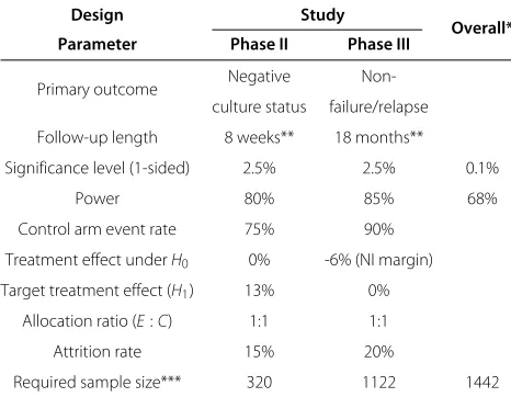
The phase II two-arm two-stage designs were based upon a recent study by Dorman et al. [10] that sub-stituted moxifloxacin for isoniazid in the standard TB regimen during the intensive phase (first two months) of treatment. The outcome in this study was culture status (a marker for whether a patient has TB or not) 8 weeks after randomisation and was also used as the basis for the intermediate outcome in the seamless phase II/III designs. The phase III aspect was based on the ongoing REMox TB trial (controlled comparison of two moxi-floxacin containing treatment shortening regimens in pul-monary tuberculosis) that investigates the effect of two four month regimens against the standard six month regi-men on relapse rates 18 months after randomisation [20]. This trial uses a Bonferroni-adjusted one-sided signifi-cance level of 1.25% for each treatment arm to ensure the overall type I error rate is no higher than 2.5%. For this example we considered only one experimental arm from REMox and thus used a one-sided significance level of 2.5%. The designs of these standalone phase II and phase III trials are summarised in Table 1.
Examples of two-arm two-stage phase II and phase II/III TB trials were generated using a conventional significance level (2.5%) and power (90%) in the final stage. Signifi-cance levels of 20% and 50% and powers of 90% and 95% were explored in the first stage. Delays of 4 and 14 weeks for observing a patient’s culture status after randomisation
Table 1 Design parameters for phase II and III TB trials
Design Study
Overall* Parameter Phase II Phase III
Primary outcome Negative Non-culture status failure/relapse
Follow-up length 8 weeks** 18 months**
Significance level (1-sided) 2.5% 2.5% 0.1%
Power 80% 85% 68%
Control arm event rate 75% 90%
Treatment effect underH0 0% -6% (NI margin)
Target treatment effect (H1) 13% 0%
Allocation ratio (E:C) 1:1 1:1
Attrition rate 15% 20%
Required sample size*** 320 1122 1442
Design parameters for a phase II (based on Dorman et al. [10]) and a phase III (based on REMox [20]) TB trial. *Calculated assuming independence between trials. **An additional 6 week delay is typically required to determine culture status. ***Sample sizes estimated using equations (1) and (2). NI = non-inferiority.
were used to explore their effect on the efficiency of a trial. The latter was chosen as it is the current delay in observ-ing a patient’s culture status after randomisation due to the 8 week follow-up period plus 6 week wait for detect-ing absence of TB (in liquid medium). A 4 week delay was also chosen as it is not yet certain whether culture sta-tus at 8 weeks is an appropriate intermediate outcome for long-term relapse, and observing it after 4 weeks may be more suitable. Furthermore, the 6 week wait is unlikely to exist in future as techniques for immediate detection of TB are developed [21] and so observing status at 4 weeks may represent the shortest possible delay for this outcome. Examples of two-arm two-stage phase II and phase II/III TB trial designs based on these parameters are shown in Tables 2 and 3 respectively and discussed in the ‘Results’ section.
The efficiency of each design was measured by its expected sample size (ESS), that is, the mean number of patients recruited to the trial before it is terminated [22], calculated under the null hypothesis. ESS was compared between designs with roughly similar overall operating characteristics to determine which is likely to require fewer resources when the experimental treatment is inef-fective. For a single-stage trial, such as those in Table 1, the ESS is equal to the overall sample size since there is no opportunity for stopping before the planned end of the trial (except perhaps in extreme circumstances such as overwhelming efficacy of an arm).
To calculate the overall operating characteristics in the seamless designs an estimate of the positive predictive value, that is, the probability of a patient not relapsing or being classed as a treatment failure given that they have a negative culture, was obtained from a meta-analysis by Horne et al. [23] who estimated it to be 95% (95% CI (95%, 96%)) for cultures taken at 2 months. This value was assumed to be the same underH0andH1 for each intermediate outcome.
Simulation study
Table 2 Examples of two-arm two-stage phase II TB trials
Design Stage (i) αi ωi
Length of f/u = 4 weeks Length of f/u = 8 weeks*
ρ Ai i
Fixed
ni Ni ti ESS|H0 ni Ni ti ESS|H0 sample size
(i) 1 0.5 0.90 56 96 0.48 262 56 134 0.67 281 0.39 0.500 0.900 360
2 0.025 0.90 364 428 2.30 364 428 2.49 0.021 0.826
(ii) 1 0.5 0.95 94 140 0.70 284 94 178 0.89 303 0.51 0.500 0.950 398
2 0.025 0.90 364 428 2.30 364 428 2.49 0.023 0.870
(iii) 1 0.2 0.90 156 214 1.07 257 156 252 1.26 287 0.65 0.200 0.900 381
2 0.025 0.90 364 428 2.30 364 428 2.49 0.020 0.843
(iv) 1 0.2 0.95 214 282 1.41 311 214 320 1.60 342 0.77 0.200 0.950 414
2 0.025 0.90 364 428 2.30 364 428 2.49 0.023 0.883
Characteristics of two-arm two-stage TB trials whereI=D= culture status observed 4 or 14 weeks after randomisation. The fixed sample sizes correspond to fixed sample designs with pairwise alphaA2and power 2. Key: for stagei,αi= significance level,ωi= nominal power,ni= total sample size required for analysisi,Ni=
cumulative number of patients recruited by the end of stagei,ti= predicted timing (in years) of the end of stageiassuming a recruitment rate of 200 patients/year,
ESS|H0= expected sample size under the null hypothesis,ρ= correlation between stages,Ai= probability of passing stageiunderH0, i= probability of passing
stageiunderH1. *Plus an additional 6 week delay to determine culture status.
In the time-to-event case, interim analyses occur when a pre-specified number of events have been observed in the control arm. In arms in which recruitment is stopped early there is scope for continuing to follow-up patients who have not yet experienced the event(s) of interest and including them in a reanalysis at the planned end of the trial to obtain a less biased estimate of the treat-ment effect. This is also applicable when outcomes are observed at the end of a fixed follow-up period since not all patients will have had both their intermediate and definitive outcomes observed by each interim analysis.
A simulation study was conducted using the two-stage phase II and phase II/III TB trial designs shown in Tables 2 and 3 respectively, to quantify the bias of treatment effects estimated on the definitive outcome at:
(a) The first interim analysis in arms which are not continued to the second stage
(b) A reanalysis of the same arms (against all control arm patients recruited concurrently) after intermediate and definitive outcome data have been obtained from all patients
(c) The final stage analysis of all arms which pass all intermediate stages
Phase II/III designs in which the follow-up period forI was 4 weeks rather than the current 14 weeks (designs not shown) were also used to investigate the effect of follow-up length in (b).
In addition to bias, the proportion of arms for which recruitment is stopped at the first interim analysis and the proportion which continue recruiting to the final stage of the trial, as well as the pairwise type I error rate, power and correlation between stages were determined in the sim-ulations and compared to their corresponding calculated values.
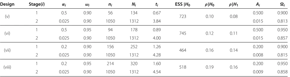
Table 3 Examples of two-arm two-stage phase II/III TB trials
Design Stage(i) αi ωi ni Ni ti ESS|H0 ρ|H0 ρ|H1 Ai i
(v) 1 0.5 0.90 56 134 0.67 723 0.10 0.08 0.500 0.900
2 0.025 0.90 1050 1312 3.84 0.015 0.813
(vi) 1 0.5 0.95 94 178 0.89 745 0.12 0.11 0.500 0.950
2 0.025 0.90 1050 1312 4.00 0.015 0.857
(vii) 1 0.2 0.90 156 252 1.26 464 0.16 0.14 0.200 0.900
2 0.025 0.90 1050 1312 4.28 0.008 0.815
(viii) 1 0.2 0.95 214 320 1.60 518 0.19 0.16 0.200 0.950
2 0.025 0.90 1050 1312 4.54 0.009 0.858
Characteristics of two-arm two-stage TB trials whereI= culture status observed 14 weeks after randomisation andD= relapse status at 18 months. Key: for stagei,αi=
significance level,ωi= nominal power,ni= total sample size required for analysisi,Ni= cumulative number of patients recruited by the end of stagei,ti= predicted
timing (in years) of the end of stagei, ESS|H0= expected sample size under the null hypothesis,ρ|Hh= correlation between stages under hypothesisHh,Ai=
For each design shown in Tables 2 and 3, the bias associ-ated with the following four pairs of underlying treatment effects for the culture status (CS) and relapse outcomes (R) were investigated in the simulations:
A. θCS= −5%,θR= −10%(treatment effects worse than those underH0)
B. θCS=0%,θR= −6%(treatment effects underH0
(see Table 1))
C. θCS=8%,θR= −3%(treatment effects between those underH0andH1)
D. θCS=13%,θR=0%(treatment effects underH1(see
Table 1))
By assessing bias in scenarios (a), (b) and (c) for this variety of treatment effects, recommendations can be made for designing multi-stage trials which reduce bias, thus improving the accuracy of treatment effect esti-mates which might be used, for example, in future meta-analyses, policy-making decisions or the design of future trials.
Simulation methods
To perform the bias assessment and assess the accuracy of the calculation of the pairwise operating characteris-tics, individual patient data were simulated for each phase II and phase II/III design under treatment effects A-D. In each case 40,000 replicates were generated to estimate pass/fail rates to an accuracy of at least 0.5% at the 5% significance level. For each patient, missing value indica-tors for theIandDoutcomes were drawn from Bernoulli distributions with parameters derived from Table 1. In the designs where I = D the probability of observing the definitive outcome was not conditional on observ-ing the intermediate outcome. Although this reduces the correlation between stages compared to the calculation given in the appendix where all patients with a missing intermediate outcome are also assumed to have a missing definitive outcome, these different assumptions will indi-cate the robustness of the calculation of the overall type I error rate and power.
Patient outcomes were drawn from Bernoulli distribu-tions with control arm event rates derived from Table 1. The underlying event rates for experimental arms with underlying effects A-D were found by adding on the corre-sponding treatment effects shown above. Since the phase III outcome (relapse) is dependent on culture status, the event rate will differ according to whether a patient’s cul-ture status is positive (CS=0), negative (CS=1) or miss-ing. The positive predictive value (PPV=P(R=1|CS=1)) is the relapse event rate for patients with a positive culture status and the estimate from Horne et al. (95%) [23] was assumed for all arms. The probabilityP(R = 1|CS = 0)
for each treatment arm was then found by rearranging the formula
P(R=1)=P(R=1|CS=1)P(CS=1)
+P(R=1|CS=0)P(CS=0)
Unconditional event rates were used for patients with missing intermediate outcomes.
When simulating each trial, analyses were triggered once the pre-determined number of control arm patients had their outcome of interest observed. The pairwise type I error rate and power for each design was cal-culated as the proportion of arms simulated under H0 (treatment arm B) andH1(treatment arm D) respectively which passed all stages of the trial. For each underly-ing treatment effect in each design, the absolute bias in scenarios (a), (b) and (c) was calculated as the average deviation of all treatment effect estimates from the true value.
Results
Examples of phase II TB trials
Table 2 summarises the sample sizes and durations of phase II two-arm two-stage trials which use culture sta-tus at 4 or 8 weeks of follow-up as the primary endpoint for both the intermediate and definitive outcomes. A con-stant recruitment rate of 200 patients/year was assumed in both stages.
The results show that the maximum sample sizes of the two-stage designs shown in Table 2 are higher than the corresponding fixed sample sizes, however, their expected sample sizes are much lower as they allow recruitment to be stopped early if the experimental treatment does not show sufficient benefit at the first stage. Increasing the power in the first stage reduces the difference between the maximum and fixed sample sizes, however, this also increases the expected sample sizes due to a larger first stage. Thus, a balance needs to be found between the two measures. As expected, the correlation between stages increases as the gap between analyses decreases, however, this only marginally increases the type I error rate and power.
There appears little advantage in using these two-stage designs over a single-stage design for two-arm phase II TB trials, however, if multiple treatments are to be evaluated in a single trial then stopping guidelines for lack-of-benefit will become much more useful. Due to the current length of follow-up for culture status (8 weeks) and short length of phase II trials, using more than two-stages is unlikely to improve efficiency.
Examples of seamless phase II/III TB trials
Examples of seamless two-stage TB trials are presented in Table 3. A constant recruitment rate of 200 patients/year was assumed for the intermediate (phase II) stage and a much higher recruitment rate of 800 patients/year was used for the second (phase III) stage. Under these assump-tions the maximum duration of each design is no longer than 5 years. If similar recruitment rates are assumed for the fixed sample designs shown in Table 1 then the maximum duration of conducting both trials separately is approximately 8.5 years assuming a modest delay between phases of 3 years. Furthermore, the overall power of the seamless designs (over 80%) is much higher than that for conducting trials separately (68%) and maximum sample sizes are over 100 patients lower.
The between-stage correlations in these designs are much lower than those in the phase II designs for two rea-sons. Firstly, the positive predictive value is effectively 1 in designs withI = D(see Appendix) whereas the seam-less designs use a slightly lower value (0.95). Secondly, the interim and final analyses are much further apart in terms of sample size than in the phase II designs, which fur-ther reduces the correlation. Although not problematic, the immediate consequence of lower between-stage cor-relation is a reduction in both the pairwise type I error rate and power, and so the stagewise operating characteristics may have to be increased to achieved the desired level for each measure.
A downside of the seamless designs presented in Table 3, as illustrated by the high ESS, is that ineffective arms have a reasonable chance of proceeding to the final stage of the trial due to the high significance level used in the first stage. To combat this, the large gap between the first and final analyses means that an extra inter-mediate stage could be added to the trial. For exam-ple, adding a second intermediate stage with 95% power and a 10% significance level to design (vi) in Table 3 reduces the ESS to 377 with only a 3% reduction in overall power. This loss can be recovered by slightly increasing the stagewise powers. Identifying MAMS designs which maintain the overall operating characteris-tics but have desirable properties such as minimising the expected or maximum sample sizes is an area of ongoing research.
Clearly there is much more benefit in using the MAMS design for seamless phase II/III TB trials than for phase II alone. We have demonstrated the savings in time and resources that can be achieved in using seamless two-arm two-stage trials over conducting each phase separately. For multi-arm multi-stage seamless trials, the savings will potentially be much greater compared to conducting sep-arate phase II and phase III trials for each experimental treatment.
Results of simulation study
Table 4 shows that the overall type I error rate, power and correlation between stages estimated from the simulations of the designs shown in Tables 2 and 3 agree very well with the corresponding calculated values. As expected, when I =Dthe correlation between stages estimated from the simulations is slightly lower than the calculated values, however, this leads to only a negligible difference between the overall type I error rates and powers showing that the calculation is robust to the degree of dependence between observing each outcome.
Bias in arms dropped at the first analysis
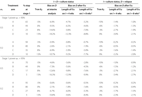
Table 5 summarises the simulation results for the pro-portion of arms dropped at the end of the first stage and the absolute bias in their treatment effect estimates on the definitive outcome at the interim analysis and after all remaining patients have completed follow-up. The pro-portion of arms dropped under H0 (treatment effect B) and H1 (treatment effect D) is as expected given the significance level and power in this stage.
The results show that, on average, treatment effects are underestimated in arms which do not show suffi-cient benefit at the first interim analysis. When I = D the absolute bias in such arms is particularly high when a high significance level (50%) and relatively low power (90%) is used (design (i) in Table 2), in other words, the earlier the interim analysis occurs. In this design the magnitude of the absolute bias is over 9% under H0. However, the bias is markedly reduced in a reanal-ysis after all remaining patients have had their outcome observed, with a greater reduction in bias when using a longer follow-up period or, more generally, when more patients can be added to the reanalysis. In this particu-lar example, the magnitude of the absolute bias underH0 decreases from 9.5% to 6.5% for 4 week follow-up and to 4.6% if outcome observation is delayed by 14 weeks after randomisation.
Table 4 Correlations, type I error rates and powers obtained from simulation compared to calculated values
Design α1 ω1
From calculation From simulation
ρ|H0 ρ|H1 α ω ρˆ|H0 ρˆ|H1 αˆ ωˆ
I=D=culture status
(i) 0.50 0.90 0.39 0.39 0.021 0.826 0.38 0.38 0.021 0.828
(ii) 0.50 0.95 0.50 0.50 0.023 0.870 0.50 0.50 0.024 0.872
(iii) 0.20 0.90 0.65 0.65 0.020 0.843 0.64 0.65 0.019 0.847
(iv) 0.20 0.95 0.76 0.76 0.023 0.883 0.76 0.76 0.023 0.885
I= culture status,D= relapse
(v) 0.50 0.90 0.10 0.08 0.015 0.813 0.07 0.06 0.014 0.809
(vi) 0.50 0.95 0.12 0.11 0.015 0.857 0.10 0.09 0.015 0.854
(vii) 0.20 0.90 0.16 0.14 0.008 0.815 0.12 0.11 0.008 0.811
(viii) 0.20 0.95 0.19 0.16 0.009 0.858 0.15 0.12 0.008 0.858
Overall type I error rates, powers and correlations between stages obtained from simulations of designs (i)-(viii) in Tables 2 and 3. Key:α1= stage 1 significance level, ω1= stage 1 power,ρ|Hh= correlation between stages under hypothesisHh,α= overall type I error rate,ω= overall power. Hats indicate values estimated from
simulations.
Table 5 Absolute bias in arms dropped at the first interim analysis
I=D= culture status I= culture status,D= relapse
α1
Treatment % stop
TrueθD
Bias onD Bias onDafter f/u
TrueθD
Bias onDafter f/u arm at at interim Length of f/u Length of f/u Length of f/u Length of f/u
stage 1 analysis onI= 4 wks onI= 8 wks* onI= 4 wks onI= 8 wks*
Stage 1 powerω1= 90%
0.5
A 65 -5% -6.9% -4.7% -3.2% -10% -1.4% -1.0%
B 49 0% -9.5% -6.5% -4.6% -6% -1.7% -1.3%
C 23 8% -14.6% -9.8% -7.0% -3% -2.7% -1.9%
D 10 13% -18.2% -12.3% -8.8% 0% -3.0% -2.1%
0.2
A 94 -5% -0.9% -0.8% -0.7% -10% -0.2% -0.2%
B 80 0% -2.6% -2.1% -1.9% -6% -0.5% -0.5%
C 35 8% -6.9% -5.9% -5.0% -3% -1.6% -1.4%
D 10 13% -10.7% -9.2% -7.7% 0% -2.2% -2.0%
Stage 1 powerω1= 95%
0.5
A 70 -5% -4.6% -3.6% -2.8% -10% -1.0% -0.9%
B 49 0% -7.3% -5.6% -4.5% -6% -1.5% -1.2%
C 17 8% -12.6% -9.8% -7.6% -3% -2.7% -2.1%
D 5 13% -16.3% -12.9% -9.9% 0% -3.4% -2.7%
0.2
A 95 -5% -0.6% -0.6% -0.5% -10% -0.2% -0.2%
B 80 0% -2.1% -1.8% -1.6% -6% -0.5% -0.4%
C 27 8% -6.7% -6.0% -5.3% -3% -1.7% -1.5%
D 5 13% -10.8% -9.6% -8.4% 0% -2.3% -2.1%
Simulation results showing the proportion of trials stopped at the first interim analysis and the absolute bias for such arms in the estimated treatment effect onDat the interim analysis and after all remaining patients have been followed up. Key:α1= significance level in stage 1,θD= underlying treatment effect on the definitive
the bias in the treatment effect estimates for Dis much lower than when the same outcome is used throughout the trial, even when using a high significance level in the first stage.
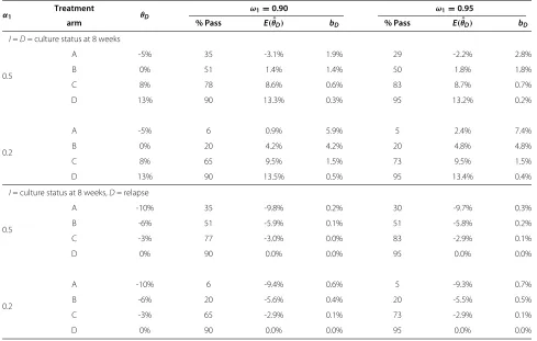
Bias in arms reaching the final analysis
Table 6 shows that treatment effects estimated at the final planned analysis of the trial are overestimated on average, although the bias is generally not as large as it is for arms dropped at the first analysis. The results suggest that bias decreases the further the interim analysis is in terms of sample size from the final analysis (i.e. as the correlation between stages decreases) and when the chance of pro-ceeding to the final stage of the trial is higher, as is the case for effective arms.
In the examples used in Table 6 the bias is practically zero in all cases whenI = D, even for ineffective arms. This is due to the very low correlation between stages in these designs (roughly 0.1). However, even when the cor-relation is higher, for example whenI=D, the bias is still approximately zero for arms which are likely to proceed
to the final stage. Bias is higher for ineffective arms, how-ever, in a well-designed MAMS trial such arms should have little chance of reaching the final stage.
Discussion
We have successfully adapted the MAMS design ini-tially developed by Royston et al. [6] to binary outcomes which are observed at the end of a fixed follow-up period and analysed using an absolute difference in pro-portions. Throughout this paper we have used TB as an example of a disease area where a MAMS approach could dramatically speed up treatment evaluation com-pared to the traditional approach of separate, two-arm phase II and III trials. Savings in time and resources are particularly large when using the MAMS design to incorporate both phase II and phase III into a sin-gle seamless trial, however, savings are still likely to be made when using it to design multi-arm phase II tri-als. Many new and repurposed drugs are currently in clinical development for TB and so a huge number of new regimens are likely to be available for testing in
Table 6 Absolute bias in arms reaching the final analysis
α1 Treatment θD
ω1=0.90 ω1=0.95
arm % Pass E(ˆθD) bD % Pass E(ˆθD) bD
I=D= culture status at 8 weeks
0.5
A -5% 35 -3.1% 1.9% 29 -2.2% 2.8%
B 0% 51 1.4% 1.4% 50 1.8% 1.8%
C 8% 78 8.6% 0.6% 83 8.7% 0.7%
D 13% 90 13.3% 0.3% 95 13.2% 0.2%
0.2
A -5% 6 0.9% 5.9% 5 2.4% 7.4%
B 0% 20 4.2% 4.2% 20 4.8% 4.8%
C 8% 65 9.5% 1.5% 73 9.5% 1.5%
D 13% 90 13.5% 0.5% 95 13.4% 0.4%
I= culture status at 8 weeks,D= relapse
0.5
A -10% 35 -9.8% 0.2% 30 -9.7% 0.3%
B -6% 51 -5.9% 0.1% 51 -5.8% 0.2%
C -3% 77 -3.0% 0.0% 83 -2.9% 0.1%
D 0% 90 0.0% 0.0% 95 0.0% 0.0%
0.2
A -10% 6 -9.4% 0.6% 5 -9.3% 0.7%
B -6% 20 -5.6% 0.4% 20 -5.5% 0.5%
C -3% 65 -2.9% 0.1% 73 -2.9% 0.1%
D 0% 90 0.0% 0.0% 95 0.0% 0.0%
Simulation results showing the proportion of trials which continue to the final stage of the trial (% pass) and the absolute bias in the estimated treatment effect onD
at the final analysis. Key:θD= underlying treatment effect on the definitive outcome,α1= significance level in stage 1,ω1= nominal power in stage 1,E(θˆD)= average
treatment effect on the definitive outcome in the final stage,bD=E(θˆD)−θD= bias in the average treatment effect estimate on the definitive outcome in the final
phase II and III trials in the near future. Evaluating them in separate, single stage trials will not only be costly but will prolong the discovery of a simpler and shorter effective regimen by decades. Use of novel trial designs such as the MAMS design is therefore urgently required.
Further work is needed to determine the best interme-diate outcome for long-term relapse before the MAMS design described here can be used to evaluate TB treat-ments in a seamless phase II/III trial. The methods used by Barthel et al. [14], who evaluated the perfor-mance of the MAMS design for time-to-event outcomes in four cancer trials, could be applied to past TB tri-als. If the rate at which trials are incorrectly stopped for lack-of-benefit on culture status at eight weeks is high then other intermediate outcomes will need con-sidering, such as culture status at other time points. Another candidate for the intermediate outcome is time to culture conversion, which is increasingly being used in phase II trials and is arguably a more reliable surro-gate endpoint than culture status at a single time point [24]. Although surrogacy is not a requirement for an intermediate outcome it is likely that a surrogate out-come will be a reliable choice. An ongoing trial con-ducted by the PanACEA consortium with a MAMS design (ClinicalTrials.gov identifier NCT01785186) is using this endpoint but since this is a phase II trial the definitive outcome is also time to culture conver-sion. Incorporating this outcome into a MAMS design with a binary definitive outcome will require further extensions to the methodology which we are currently developing.
The amount of bias likely to be generated in various examples of phase II and phase II/III TB trials was inves-tigated and was shown to be of no practical importance in arms reaching the final analysis, particularly in effective arms or when treatment selection is based on an inter-mediate outcome. In general, the bias at the final analysis increases as the treatment effects estimated at each stage become more correlated. This is caused by having short stage durations in which only a small amount of new data can be collected. Ensuring that stages are adequately spaced is not only practical from the perspective of every-one involved in the trial but it will also limit the amount of bias likely to be generated.
As shown by Choodari-Oskooei et al. [15], we also found that having an early first interim analysis increased the bias of treatment effect estimates in arms dropped at this analysis, particularly when the intermediate and definitive outcomes were identical. Bias was markedly reduced in a reanalysis after all patients had completed follow-up. It should be noted, however, that the aver-age treatment effect in arms which are stopped early for lack-of-benefit (i.e. are statistically non-significant) will
necessarily appear less effective than their true value [25]. Freidlin and Korn [26] suggest that the most appropri-ate comparator for the x% of trials stopped at the first interim analysis is the average treatment effect estimate of the same outcome in the correspondingx% most extreme trials in the fixed sample-size design (the design that has no interim analyses). When taking this into consideration the bias estimates in Table 5 are nearly halved (data not shown).
A calculation for the overall type I error rate for a sin-gle experimental arm was described, thus allowing control of this measure. However, in a multi-arm trial it may be more important to control the familywise type I error rate (FWER), that is, the probability of rejecting at least one true null hypothesis at the end of the trial. Freidlin et al. [7] argue that this decision depends on the clinical questions that the trial is addressing. For example, if a multi-armed trial was used purely for efficiency reasons and the inter-pretation of the results of one arm has no influence over the results of other arms then they argue that no control of the FWER needs to be made. On the other hand, if in some way the treatment arms are related, such as different doses or schedules of the same treatment, then multiplic-ity adjustment should be made. Others have said that if a multi-arm design is to be used in a confirmatory trial then FWER control is a requirement [27,28].
For the MAMS design described here, a crude method for ensuring that the FWER is no higher than some pre-specified level is to apply a Bonferonni correction to the pairwise type I error rate: i.e. in a trial withK experimen-tal arms, a pairwiseα equal to FWER/K could be used. However, such a correction can be too conservative and may result in a trial which is much larger than might be necessary, thus losing efficiency. More accurate methods for controlling the FWER in the strong sense (i.e. under any parameter configuration) are therefore required and is a subject of ongoing research. Alternatively, other MAMS designs which allow stopping for lack-of-benefit and control the FWER are available [29-32].
Conclusions
Appendix
Appendix: Estimating the correlation matrices
Before Ai and i can be calculated the correlation matrices,R0i andR1i, whose(j,k)th entries are the correla-tions between the treatment effects in stagesjandkunder H0andH1respectively, are required. We begin with a gen-eral case where the binary outcomes of interest in stagesj andkare different. Suppose outcomeXis the outcome of interest in stagejand outcomeY is of interest in stagek withj < kand denote the observed treatment effects by
ˆ
θj= ˆπjE− ˆπjCandθˆk = ˆπkE− ˆπkCrespectively.
Ifπih = πiC +θihis the target experimental arm event rate under hypothesisHhthen the standard deviation of θihin its normal approximation is
σih= πih
1−πih
AnCi +
πiC
1−πiC
nCi
Assuming success rates between treatment arms are independent, the correlation between θˆj and θˆk under hypothesisHh(h=0, 1), denoted byρh(j,k), is
ρh(j,k)= Cov(θˆj,θˆk) σjhσkh
= Cov
ˆ
πjh− ˆπjC,πˆkh− ˆπkC
σjhσkh
= Cov
ˆ
πjh,πˆkh +Cov
ˆ
πjC,πˆkC
σjhσkh
Denote by XmC and YmC the observed X and Y out-comes respectively for the mth patient in the control arm (XmC,YmC ∈ {0, 1}) whereXCm is observed during or before stagejandYC
m is observed during or before stage
k(j< k). The covariance between the control arm event rates in stagejon theX outcome and stagek on theY outcome is
Cov(πˆjC,πˆkC)=Cov ⎛ ⎜ ⎝ 1
nCj
nC j
l=1 XlC, 1
nCk
nCk
m=1 YmC
⎞ ⎟ ⎠
= 1 nCjnCk
nCj
l=1
nC k
m=1
CovXlC,YmC
= 1 nCjnCk
nCj
l=1
nC k
m=1
E(XlCYmC)−E(XlC)E(YmC)
Assuming observations from different patients are inde-pendent implies E(XlCYmC) = E(XlC)E(YmC) ifl = mand so
Cov(πˆjC,πˆkC)= 1
nCj nCk
nCj
l=1
E(XlCYlC)−E(XlC)E(YlC)
sincej<k
= 1 nCj nCk
nCj
l=1
π(Cj,k)−πjCπkC
= 1 nCk
π(Cj,k)−πjCπkC
whereπ(Cj,k) is the probability of a patient experiencing both theXandY outcomes in the control arm. A similar argument for the covariance of event rates between stages in an experimental arm underHhgives
Cov
ˆ
πjE,πˆkE = 1
AnCk
π(hj,k)−πjhπkh . It follows that
ρ(hj,k)=
π(hj,k)−πjhπkh +A
π(Cj,k)−πjCπkC
AnCkσjhσkh (3)
The valuesπ(Cj,k)andπ(hj,k)may be estimated from prior knowledge or, if estimates of the positive predictive value in each arm are available, that is, the probability of a patient having aY event given that they have had anX event, then from the definition of conditional probability
π(Cj,k)=PYmC =1|XmC =1 πjC and
π(hj,k)=P
Ymh =1|Xhm=1 πjC.
If the outcomes of interest in stagesjandkare the same then equation (3) simplifies. Clearly the positive predictive value is now 1 and soπ(Cj,k)=πjCandπ(hj,k)=πjh. Then
ρ(hj,k)=
πjh−(πjh)2 +AπjC−(πjC)2
AnCkσjhσkh
= π
h j
1−πjh +AπjC
1−πjC
AnCkσjhσkh
= n
C j
σjh 2
nCkσjhσkh = nCj
since underlying treatment effects are assumed to be con-stant throughout the trial. Note that these correlations are the same underH0andH1(ρ(0j,k)=ρ(1j,k)).
The entries,ρ(hj,k), below the main diagonal of the cor-relation matrices can now be calculated using (3) for the correlations between the intermediate and final outcomes and (4) for the correlations between the intermediate out-come in different stages. Since each matrix is symmetric we setρ(hj,k) = ρ(hk,j)and all diagonal entries, i.e. the cor-relation between treatment effects in the same stage, are ρ(hj,j)=1.
Abbreviations
MAMS: Multi-arm multi-stage; TB: Tuberculosis; ESS: Expected sample size; FWER: Familywise error rate.
Competing interests
The authors declare that they have no competing interests.
Authors’ contributions
DJB drafted the manuscript, carried out the mathematical calculations and performed the simulations. All authors read and approved the final manuscript.
Acknowledgements
We would like to thank Brennan Kahan and the reviewers for their useful comments which have helped to improve this manuscript.
Received: 26 April 2013 Accepted: 25 October 2013 Published: 14 November 2013
References
1. US Food and Drug Administration:Innovation or stagnation: challenge and opportunity on the critical path to new medical products. Tech. rep., US Dept of Health and Human Services 2004.
2. Ma Z, Lienhardt C, McIlleron H, Nunn AJ, Wang X:Global tuberculosis drug development pipeline: the need and the reality.Lancet2010, 375(9731):2100–2109.
3. Lienhardt C, Raviglione M, Spigelman M, Hafner R, Jaramillo E, Hoelscher M, Zumla A, Gheuens J:New drugs for the treatment of tuberculosis: needs, challenges, promise, and prospects for the future.J Infect Dis
2012,205(suppl 2):S241–S249.
4. World Health Organisation:WHO report. Global tuberculosis control. Geneva: World Health Organisation; 2011.
5. Phillips PPJ, Gillespie SH, Boeree M, Heinrich N, Aarnoutse R, McHugh T, Pletschette M, Lienhardt C, Hafner R, Mgone C, Zumla A, Nunn AJ, Hoelscher M:Innovative trial designs are practical solutions for improving the treatment of tuberculosis.J Infect Dis2012, 205(suppl 2):S250–S257.
6. Royston P, Barthel FM, Parmar MK, Choodari-Oskooei B, Isham V:Designs for clinical trials with time-to-event outcomes based on stopping guidelines for lack of benefit.Trials2011,12:81.
7. Freidlin B, Korn EL, Gray R, Martin A:Multi-arm clinical trials of new agents: some design considerations.Clin Cancer Res2008, 14(14):4368–4371.
8. Sydes MR, Parmar MK, James ND, Clarke NW, Dearnaley DP, Mason MD, Morgan RC, Sanders K, Royston P:Issues in applying multi-arm multi-stage methodology to a clinical trial in prostate cancer: the MRC STAMPEDE trial.Trials2009,10:39.
9. Parmar MK, Barthel FM, Sydes M, Langley R, Kaplan R, Eisenhauer E, Brady M, James N, Bookman MA, Swart AM, Qian W, Royston P:Speeding up the evaluation of new agents in cancer.J Natl Cancer Inst2008, 100(17):1204–1214.
10. Dorman SE, Johnson JL, Goldberg S, Muzanye G, Padayatchi N, Bozeman L, Heilig CM, Bernardo J, Choudhri S, Grosset JH, Guy E, Guyadeen P, Leus
MC, Maltas G, Menzies D, Nuermberger EL, Villarino M, Vernon A, Chaisson RE:Substitution of moxifloxacin for isoniazid during intensive phase treatment of pulmonary tuberculosis.Am J Respir Crit Care Med2009, 180(3):273–280.
11. Burman WJ, Goldberg S, Johnson JL, Muzanye G, Engle M, Mosher AW, Choudhri S, Daley CL, Munsiff SS, Zhao Z, Vernon A, Chaisson RE: Moxifloxacin versus ethambutol in the first 2 months of treatment for pulmonary tuberculosis.Am J Respir Crit Care Med2006, 174(3):331–338.
12. Conde MB, Efron A, Loredo C, De Souza GR, Graca NP, Cezar MC, Ram M, Chaudhary MA, Bishai WR, Kritski AL, Chaisson RE:Moxifloxacin versus ethambutol in the initial treatment of tuberculosis: a double-blind, randomised, controlled phase II trial.Lancet2009,
373(9670):1183–1189.
13. Phillips PP, Nunn AJ:Challenges of phase III study design for trials of new drug regimens for the treatment of TB.Future Med Chem2010, 2(8):1273–1282.
14. Barthel FM, Parmar MK, Royston P:How do multi-stage, multi-arm trials compare to the traditional two-arm parallel group design–a reanalysis of 4 trials.Trials2009,10:21.
15. Choodari-Oskooei B, Parmar MKB, Royston P, Bowden J:Impact of lack-of-benefit stopping rules on treatment effect estiamtes of two-arm multi-stage (TAMS) trials with time to event outcome. Trials2013,14:23.
16. Blackwelder WC:“Proving the null hypothesis” in clinical trials. Control Clin Trials1982,3(4):345–53.
17. Machin D, Campbell MJ, Tan SB, Tan SH:Sample Size Tables for Clinical Studies: Wiley-Blackwell; 2009.
18. Little RJ, D’Agostino R, Cohen ML, Dickersin K, Emerson SS, Farrar JT, Frangakis C, Hogan JW, Molenberghs G, Murphy SA, Neaton JD, Rotnitzky A, Scharfstein D, Shih WJ, Siegel JP, Stern H:The prevention and treatment of missing data in clinical trials.N Engl J Med2012, 367(14):1355–1360.
19. Korn EL, Freidlin B, Abrams JS, Halabi S:Design issues in randomized phase II/III trials.J Clin Oncol2012,30(6):667–671.
20. Nunn AJ, Phillips PP, Gillespie SH:Design issues in pivotal drug trials for drug sensitive tuberculosis (TB).Tuberculosis2008,
88(Suppl 1):S85–S92.
21. McNerney R, Maeurer M, Abubakar I, Marais B, Mchugh TD, Ford N, Weyer K, Lawn S, Grobusch MP, Memish Z, Squire SB, Pantaleo G, Chakaya J, Casenghi M, Migliori GB, Mwaba P, Zijenah L, Hoelscher M, Cox H, Swaminathan S, Kim PS, Schito M, Harari A, Bates M, Schwank S, O’Grady J, Pletschette M, Ditui L, Atun R, Zumla A:Tuberculosis diagnostics and biomarkers: needs, challenges, recent advances, and opportunities. J Infect Dis2012,205(suppl 2):S147–S158.
22. Wason JM, Jaki T:Optimal design of multi-arm multi-stage trials. Stat Med2012,31(30):4269–4279.
23. Horne DJ, Royce SE, Gooze L, Narita M, Hopewell PC, Nahid P, Steingart KR:Sputum monitoring during tuberculosis treatment for predicting outcome: systematic review and meta-analysis. Lancet Infect Dis2010,10(6):387–394.
24. Davies GR:Early clinical development of anti-tuberculosis drugs: science, statistics and sterilizing activity.Tuberculosis (Edinb)2010, 90(3):171–176.
25. Goodman SN:Stopping at nothing? some Dilemmas of data monitoring in clinical trials.Ann Intern Med2007,146(12):882–887. 26. Freidlin B, Korn EL:Stopping clinical trials early for benefit: impact on
estimation.Clin Trials2009,6(2):119–125.
27. Wason J, Magirr D, Law M, Jaki T:Some recommendations for multi-arm multi-stage trials.Stat Methods Med Res2012. doi:10.1177/0962280212465498.
28. Committee for propriertary medicinal products:Points to consider on multiplicity issues in clinical trials.Tech. rep., EMEA 2002.
29. Friede T, Parsons N, Stallard N, Todd S, Valdes Marquez E, Chataway J, Nicholas R:Designing a seamless phase II/III clinical trial using early outcomes for treatment selection: an application in multiple sclerosis.Stat Med2011,30(13):1528–1540.
31. Magirr D, Jaki T, Whitehead J:A generalized Dunnett test for multi-arm multi-stage clinical studies with treatment selection.Biometrika2012, 99(2):494–501.
32. Jaki T, Magirr D:Considerations on covariates and endpoints in multi-arm multi-stage clinical trials selecting all promising treatments.Stat Med2013,32(7):1150–1163.
doi:10.1186/1471-2288-13-139
Cite this article as:Brattonet al.:A multi-arm multi-stage clinical trial design for binary outcomes with application to tuberculosis.BMC Medical Research Methodology201313:139.
Submit your next manuscript to BioMed Central and take full advantage of:
• Convenient online submission
• Thorough peer review
• No space constraints or color figure charges
• Immediate publication on acceptance
• Inclusion in PubMed, CAS, Scopus and Google Scholar
• Research which is freely available for redistribution