Evaluation of exposure-specific risks from two independent samples: A simulation study

(1)

R E S E A R C H A R T I C L E

Open Access

Evaluation of exposure-specific risks from two

independent samples: A simulation study

William M Reichmann

1,2*

, David Gagnon

2,4

, C Robert Horsburgh

3

, Elena Losina

1,2

Abstract

Background:Previous studies have proposed a simple product-based estimator for calculating exposure-specific risks (ESR), but the methodology has not been rigorously evaluated. The goal of our study was to evaluate the existing methodology for calculating the ESR, propose an improved point estimator, and propose variance estimates that will allow the calculation of confidence intervals (CIs).

Methods:We conducted a simulation study to test the performance of two estimators and their associated confidence intervals: 1) current (simple product-based estimator) and 2) proposed revision (revised product-based estimator). The first method for ESR estimation was based on multiplying a relative risk (RR) of disease given a certain exposure by an overall risk of disease. The second method, which is proposed in this paper, was based on estimates of the risk of disease in the unexposed. We then multiply the updated risk by the RR to get the revised product-based estimator. A log-based variance was calculated for both estimators. Also, a binomial-based variance was calculated for the revised product-based estimator. 95% CIs were calculated based on these variance

estimates. Accuracy of point estimators was evaluated by comparing observed relative bias (percent deviation from the true estimate). Interval estimators were evaluated by coverage probabilities and expected length of the 95% CI, given coverage. We evaluated these estimators across a wide range of exposure probabilities, disease probabilities, relative risks, and sample sizes.

Results:We observed more bias and lower coverage probability when using the existing methodology. The revised product-based point estimator exhibited little observed relative bias (max: 4.0%) compared to the simple product-based estimator (max: 93.9%). Because the simple product-based estimator was biased, 95% CIs around this estimate exhibited small coverage probabilities. The 95% CI around the revised product-based estimator from the log-based variance provided better coverage in most situations.

Conclusion:The currently accepted simple product-based method was only a reasonable approach when the exposure probability is small (< 0.05) and the RR is≤3.0. The revised product-based estimator provides much improved accuracy.

Background

Exposure-specific risk (ESR) is defined as the risk of dis-ease (or any outcome) given a specific exposure (or sub-group). ESRs are useful to clinicians because it allows a much more meaningful way of explaining risk to patients. They are also useful to investigators who are looking to use ESRs for their own work, which may include publishing their own work or planning studies. In the absence of having access to the primary data or a

reported estimate of the ESR in the literature, the ESR can be estimated from two independent samples if the investigator knows the overall risk of disease and the relative risk (RR) of disease given the exposure of inter-est. There have been a number of published studies where ESRs have been calculated from two independent samples by multiplying the overall risk of disease from one sample by the RR from a second independent sam-ple [1,2]. Stewart et al. computed the ESR of hip fracture given certain exposures (prior fracture, family history of fracture, low body weight, and smoking) in persons over the age of 70 in the United Kingdom [2]. This study found that the ESR of hip fracture among those with all * Correspondence: [email protected]

1

Department of Orthopedic Surgery, Brigham and Women’s Hospital, 75 Francis Street, Boston, MA 02115, USA

Full list of author information is available at the end of the article

(2)

4 exposures was 8.9%. This was done by multiplying an overall risk of hip fracture of 1.91% by a RR of 4.66 [2].

Horsburgh computed the ESR of tuberculosis for mul-tiple risk factors, along with 95% confidence intervals (CIs). The upper (lower) bound of the 95% CI for the ESR was calculated by multiplying the upper (lower) bound of the 95% CI for the overall risk by the upper (lower) bound of the 95% CI for the RR [1]. While there has been some work addressing the multiplication of two binomial parameters [3], to the best of our knowl-edge, there are no methodological articles evaluating the properties of the simple product-based estimator that was used in the articles by Stewart et al and Horsburgh.

In this article we set to address three objectives. The first is to evaluate the properties of the simple product-based estimator of the ESR used by Stewart et al and Horsburgh. The second objective is to propose an esti-mate of the variance of the ESR, which can subsequently be used for calculating 95% CIs. Lastly, we propose a revised product-based estimator and two variances esti-mates for the revised point estimator which are used to calculate 95% CIs.

Methods Overview

We designed and implemented a simulation study to examine the properties of two different estimators of the ESR and their 95% CIs. The two estimators we sought to evaluate (and their associated CIs) were a sim-ple product-based estimator and revised product-based estimator. Point estimators were evaluated by calculating the observed relative bias. Their 95% CIs were evaluated using coverage probabilities and expected length given coverage for a wide range of parameters, including exposure probability, probability of disease among the unexposed, the RR of disease given exposure, and the sample size.

For the purposes of this paper, D represents having disease, E represents having exposure, subscript one denotes that the quantity comes from sample one, and subscript two denotes that the quantity comes from sample two. More careful examination of the mathe-matics behind this simple product-based estimator clearly shows that the estimator is at best a crude approximation of the ESR.

P (D)*RR P (D)*P (D|E)

P (D|E P(D|E) ESR

1 2 1 2

2

= ≠ =

) (1)

To estimate the ESR, this formula needs an estimate of the risk of disease in the unexposed (P (D|E₁ )) rather than the estimate of the overall risk of disease (P1(D)).

Simple Product-Based ESR

The simple product-based ESR (denoted ESRS) is

com-puted by simply multiplying the overall probability of disease from sample one by the RR from sample two. The formula is given below.

ESR P (D)*RR P (D)*P (D|E) P (D|E

S 1 2 1 2

2

= =

) (2)

Variance and Confidence Interval for the Simple Product-Based ESR

We first propose a formula for the variance of the sim-ple product-based estimator using a natural log transfor-mation. We assumed that the covariance between ln(P1

(D)) and ln(RR2) was zero because they are estimated

from independent data sets.

Var(ln(ESR )) Var(ln(P (D)*RR )) Var(ln(P (D)) ln(RR ))

Va

S 1 2

1 2

=

= +

= rr(ln(P (D) Var(ln(RR )) 2*Cov(ln(P (D)), ln(RR ))

1 2

+ +

==Var(ln(P (D)))+Var(ln(RR )) (assuming independe

1 2

n nce) Var(ln(P (D))) 1 P (D|E)

P (D|E)*n

1 P (D|E) P (D|E 1 2 2 2E 2 2 = + − + − ))*n_2E (3)

To complete the formula for the variance of the nat-ural log ESR we need the variance of the natnat-ural log of the overall risk (Var(In(P1(D)))). This is derived below

using the delta method.

Var(ln(P (D))) 1

P (D) *Var(P (D)) 1

P (D) *

P (D)*(1-P (D)) n 1 1 2 1 1 2 1 1 = = 1 1 1 1 1 (1-P (D)) n *P (D)

=

(4)

Substituting the result of equation 4 into equation 3 and we have the final variance for the natural log of the ESR:

Var(ln(ESR )) (1-P (D)) n *P (D)

1-P (D|E) P (D|E)*n 1-P ( S 1 1 1 2 2 2E 2

= + + DD|E)

P (D|E)*n2 2E

(5)

(3)

estimating the 95% confidence interval.

95% CI=exp ln(ESR ) 1.96* Var(ln(ESR ))

(

_S ± _S

)

(6)

Revised Product-Based ESR

Note, from formula 1, we need an estimate of the risk of disease in the unexposed from sample 1 (P (D|E₁ )), rather than the estimate of the overall risk of disease (P1

(D)). Assuming that the risk of disease in the unexposed is not reported from sample 1 or sample 2, we can use the law of total probability to derive P (D|E₁ ). By the law of total probability the following formula holds.

= )) P(D|E) P(D|E)*[((RR-1)*P(E)) 1]

+

= +

(7)

Next, solving for P(D|E) gives us:

P(D|E) P(D) [((RR-1)*P(E)) 1]

=

+ (8)

Here, estimates of P1(D)), P2(E), and RR2are available in

samples one and two as denoted by the subscripts. Then the final estimate for the revised product-based ESR is

ESR P (D)

[((RR -1)*P (E)) 1] RR

R 1

2 2

=

+ * 2. (9)

Variance and Confidence Interval for the Revised Product-Based ESR

The first estimate of variance derived for the revised product-based is derived for the natural log of the esti-mate. This is done similar to the derivation for the var-iance of the natural log of ESRs shown in equation 5.

The exception is that now we need to find variance of the natural log of the probability of disease among the unexposed in sample 1.

Var(ln(ESR )) (1-P (D|E))

n *P (D|E)

1 P (D|E) P (D|E)*n 1 R 1 1 1 2 2 2E =

+ − + −−P (D|E)

P (D|E)*n

2

2 2E

(10)

Thus a 95% CI for ESRRcan be constructed using the

normal approximation shown in equation 6 by substitut-ing ESRRfor ESRSand Var(ln(ESRR)) for Var(ln(ESRS)).

Since the ESR is a probability, the second estimate of the variance derived for ESRRis based on the binomial

distribution. The variance for a binomial parameter p is

p*(1 p) n

− _{. We chose to estimate the denominator of}

this formula by multiplying the sample size from sample 1 by the exposure probability from sample 2. This pro-vides a more conservative estimate of the variance because the denominator will be smaller. The final forms of this variance and the 95% CI using a normal approxi-mation to the binomial distribution are shown below.

Var ESR ESR *(1 ESR ) n *P (E)

R R R

1 2

( )= − (11)

95% CI ESR 1.96* ESR *(1 ESR ) n *P (E)

R R R

1 2

= ± − (12)

Simulation study details

(4)

the sample size was small, we ran our simulations with a sample size of 250 for both sample 1 and sample 2 under the conditions of Scenario 4 only. We did not perform this analysis in the other three scenarios because the prevalence of exposure and disease among the unexposed was too small to provide a reliable esti-mate of the RR.

Evaluation of ESR Estimators

We calculated the estimated ESR using the simple pro-duct-based method and revised propro-duct-based method for each of the 1,000 pairs of samples. We evaluated the estimators using observed relative bias. Observed rela-tive bias was defined as the difference between the aver-age of the 1,000 estimates from the 1,000 pairs of samples and the assumed population ESR divided by the assumed population ESR. Observed relative bias can be described as the percent change from the true estimate.

Evaluation of Confidence Intervals

All 95% CIs were evaluated using coverage probabilities. The coverage probability is defined as the probability that the interval covers the assumed population ESR. For each of the 1,000 pairs of samples we determine whether the assumed population ESR falls between the lower and upper bounds of the CI. The coverage prob-ability is then determined by the number of times the interval covered divided by 1,000. Since we calculated 95% CIs, we expect that our intervals would cover 950 times out of 1,000 (95%).

Expected length given coverage was also evaluated for all of our 95% CIs. For every 95% CI that covered the true value of the ESR for a given pair of 1,000 samples, the length was calculated by subtracting the lower bound from the upper bound. We then calculated the average of these lengths to get the expected length given coverage. For example, if the coverage probability was 95.1% then 951 out of 1,000 intervals covered the true value of the ESR. Therefore the expected length given coverage is based on an Nof 951. For the purpose of comparison, we also calculated the empirical 95% CI and its length. This was done by examining the distribu-tion of the direct estimator and taking the 2.5th percen-tile to be the lower bound of the 95% CI and the 97.5th percentile to be the upper bound of the 95% CI. The

length of the empirical 95% CI was calculated by sub-tracting the 2.5thpercentile from the 97.5thpercentile.

Case Study

We tested our methodology using a case study in which we calculated the risk of symptomatic knee osteoarthri-tis (OA) in obese persons by age groups. The overall risk of symptomatic knee OA by age group was derived from Oliveria et al [4]. This article reports on one of the largest population-based studies that estimates the risk of symptomatic knee OA with a cohort of more than 130,000 members of a community health plan. The rela-tive risk of symptomatic knee OA for obese persons (1.91) and proportion obese (0.371) was derived from Niu et al [5]. This study provides one of the most cur-rent estimates of the relative risk of symptomatic knee OA by obesity status and also had a substantial sample size (N = 2,660). Since the study by Niu and colleagues only studied those ages 50-79, we limited our analysis to those ages 50-59, 60-69, and 70-79.

Results

Scenario 1: Low exposure probability (.05)/Low disease probability among unexposed (.02)

In the case where the probability of exposure was low (.05) and the probability of disease among the unex-posed was low (.02), ESRR performed better than ESRS

with respect to observed relative bias. When the RR was 1.0, the observed relative bias was near 0 for both esti-mators. However, as the RR increased the observed rela-tive bias of ESRSincreased. This increased to a high of

31.4% when the RR was 5.0 and both sample sizes were 1,000. In the same situation, ESRRexhibited an observed

relative bias of 3.4%. In general, as the RR increased in magnitude so did the observed relative bias of ESRS,

while the observed relative bias of ESRRwas not larger

than 4.0% (Table 2).

Coverage probabilities for the 95% CI of ESRSwere at

least 95% when the RR was 2.0 or less, regardless of the sample size combination. However, as the RR increased (and subsequently the observed relative bias), the cover-age probabilities began to fall below 95%. The covercover-age probability fell to 87.1% when the RR was 5.0 and both sample sizes were 5,000 (Table 3). Coverage probabilities for the 95% CI for ESRRusing a log-based variance were

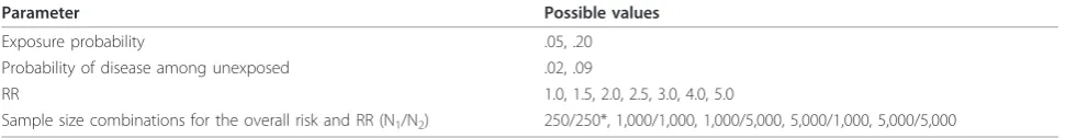
Table 1 Parameters varied and all their possible values for the simulation study

Parameter Possible values

Exposure probability .05, .20

Probability of disease among unexposed .02, .09

RR 1.0, 1.5, 2.0, 2.5, 3.0, 4.0, 5.0

Sample size combinations for the overall risk and RR (N1/N2) 250/250*, 1,000/1,000, 1,000/5,000, 5,000/1,000, 5,000/5,000

(5)

above 95% across all RRs for three of the four sample size combinations (N1 = 1,000, N2 = 1,000; N1= 5,000,

N2 = 1,000; and N1 = 5,000, N2 = 5,000). When the

sample size combination was 1,000 for the overall risk (sample 1) and 5,000 for the RR (sample 2) the 95% CI for ESRRusing a log-based variance failed to attain 95%

coverage for all RRs (see additional file 1). The exact opposite relationship was observed for the 95% CI of ESRR using a binomial variance. This interval only

attained 95% coverage when the sample size combina-tion was 1,000/5,000. In fact, these coverage probabil-ities well exceeded 95% with the smallest coverage probability being 98.9% when the RR was 1.0 (Table 4).

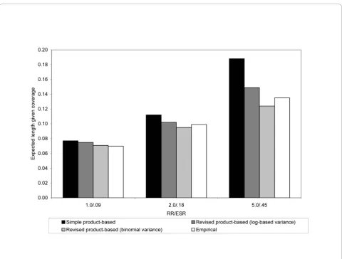
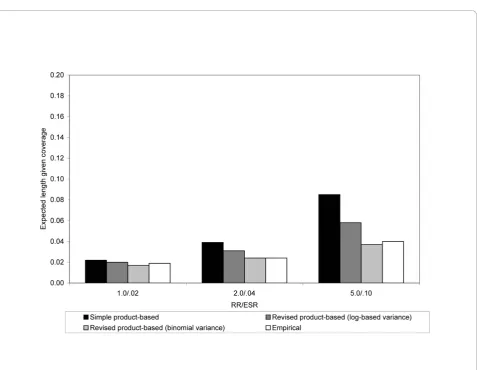
Figure 1 shows the expected lengths given coverage of all the 95% CIs constructed by different RRs (1.0, 2.0,

and 5.0 respectively) for the 5,000/5,000 (N1/N2) sample

size combination. The expected length of the empirical 95% CI is also shown. The expected length given cover-age is largest for the 95% CI around ESRS, and the

bino-mial-based variance yielded 95% CIs around ESRRwith

smaller lengths than the log-based variance 95% CIs in this scenario.

Scenario 2: Low exposure probability (.05)/Moderate disease probability among unexposed (.09)

Increasing the probability of disease among the unex-posed from .02 to .09 while keeping the exposure prob-ability set to .05 did not drastically change our results. The observed relative bias of ESRSstill increased as the

magnitude of the RR increased. When the RR was 5.0, Table 2 Observed relative bias for the simple product-based estimator (ESRS) and the revised product-based

estimator (ESRR)

Low exposure probability (.05)/Low disease probability in unexposed (.02)

N1= 1,000, N2= 1,000 N1= 5,000, N2= 5,000

RR/ESR ESRS ESRR ESRS ESRR

1.0/.02 9.5% 3.9% -1.4% -2.3%

2.0/.04 7.8% -2.6% 4.5% -1.4%

3.0/.06 18.0% 1.8% 12.2% 0.8%

4.0/.08 21.1% 0.0% 17.6% 1.1%

5.0/.10 31.4% 3.4% 22.6% 1.0%

Low exposure probability (.05)/Moderate disease probability in unexposed (.09)

N1= 1,000, N2= 1,000 N1= 5,000, N2= 5,000

1.0/.09 0.1% -0.9% 0.9% 0.6%

2.0/.18 6.1% 0.1% 5.5% 0.3%

3.0/.27 9.2% -1.4% 10.4% 0.2%

4.0/.36 16.6% 0.4% 15.9% 0.5%

5.0/.45 22.0% 0.7% 21.2% 0.8%

High exposure probability (.20)/Low disease probability in unexposed (.02)

N1= 1,000, N2= 1,000 N1= 5,000, N2= 5,000

1.0/.02 8.7% 1.1% -0.2% -1.3%

2.0/.04 26.3% -1.4% 21.4% -0.1%

3.0/.06 45.0% -1.8% 41.7% 0.1%

4.0/.08 73.3% 1.2% 61.6% 0.1%

5.0/.10 93.9% 0.3% 82.5% 0.0%

High exposure probability (.20)/Moderate disease probability in unexposed (.09)

N1= 1,000, N2= 1,000 N1= 5,000, N2= 5,000

1.0/.09 -0.8% -0.4% -1.1% -1.0%

2.0/.18 22.6% 0.7% 20.4% 0.2%

3.0/.27 40.9% -0.2% 40.3% 0.0%

4.0/.36 63.6% 0.7% 60.6% 0.1%

5.0/.45 82.6% 0.2% 81.0% 0.2%

N1is the sample the overall risk is derived from.

N2is the sample the relative risk is derived from.

(6)

the observed relative bias of ESRSwas greater than 20%

for all sample size combinations. The observed relative bias of ESRRwas close to zero for all combinations of

RR and sample size (Table 2).

Coverage probabilities for the 95% CI of ESRS were

less than 95% in most cases. The coverage probabilities were adversely affected by the increasing magnitude of the RR with a minimum coverage probability of 45% attained when the RR was 5.0 and the sample size was 5,000 for both samples (Table 3). Similar to Scenario 1, coverage probabilities for the 95% CI of ESRR using a

log-based variance exhibited at least 95% coverage in all cases except when the sample size the overall risk was derived from was 1,000 and the sample size the RR was

derived from was 5,000 (see additional file 1). The 95% CI for ESRRusing a binomial variance showed the exact

opposite relationship. Regardless of the magnitude of the RR, the coverage probability of the 95% CI for ESRR

using a binomial variance was greater than 99% when the sample size the overall risk was derived from was 1,000 and the sample size the RR was derived from was 5,000 (Table 4).

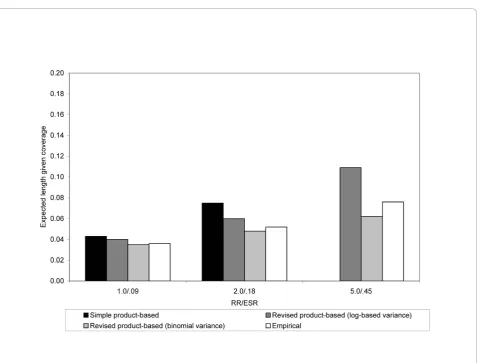
Figure 2 shows the expected lengths given coverage of the 95% CIs. The expected length given coverage increases for all the intervals as the magnitude of the RR increases. The expected lengths of the 95% CIs of ESRSand ESRR using a log-based variance are similar

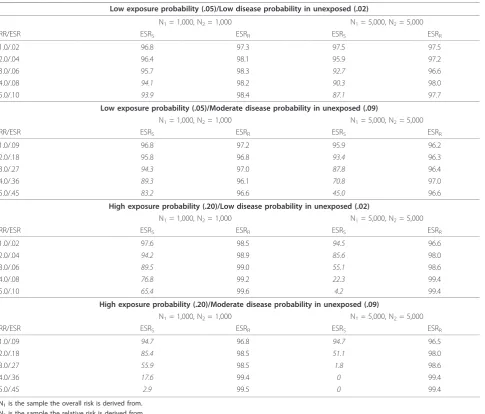
when the RR is small. However, as the RR increases in Table 3 Coverage probability for the 95% confidence interval of the simple product-based estimator (ESRS) and revised product-based estimator (ESRR) using a log-based variance

N1= 1,000, N2= 1,000 N1= 5,000, N2= 5,000

1.0/.02 96.8 97.3 97.5 97.5

2.0/.04 96.4 98.1 95.9 97.2

3.0/.06 95.7 98.3 92.7 96.6

4.0/.08 94.1 98.2 90.3 98.0

5.0/.10 93.9 98.4 87.1 97.7

Low exposure probability (.05)/Moderate disease probability in unexposed (.09)

N1= 1,000, N2= 1,000 N1= 5,000, N2= 5,000

1.0/.09 96.8 97.2 95.9 96.2

2.0/.18 95.8 96.8 93.4 96.3

3.0/.27 94.3 97.0 87.8 96.4

4.0/.36 89.3 96.1 70.8 97.0

5.0/.45 83.2 96.6 45.0 96.6

High exposure probability (.20)/Low disease probability in unexposed (.02)

N1= 1,000, N2= 1,000 N1= 5,000, N2= 5,000

1.0/.02 97.6 98.5 94.5 96.6

2.0/.04 94.2 98.9 85.6 98.0

3.0/.06 89.5 99.0 55.1 98.6

4.0/.08 76.8 99.2 22.3 99.4

5.0/.10 65.4 99.6 4.2 99.4

High exposure probability (.20)/Moderate disease probability in unexposed (.09)

N1= 1,000, N2= 1,000 N1= 5,000, N2= 5,000

1.0/.09 94.7 96.8 94.7 96.5

2.0/.18 85.4 98.5 51.1 98.0

3.0/.27 55.9 98.5 1.8 98.6

4.0/.36 17.6 99.4 0 99.4

5.0/.45 2.9 99.5 0 99.4

(7)

magnitude, the length of the 95% CI for ESRSis greater

than the length of the 95% CI for ESRR using a

log-based variance.

Scenario 3: High exposure probability (.20)/Low disease probability among unexposed (.02)

Increasing the exposure probability from .05 to .20 while the probability of disease among the unexposed was .02 affected the results substantially for the existing metho-dology. The observed relative bias of ESRSwas over 10%

when the RR was 1.5, over 20% when the RR was 2.0, and over 80% when the RR was 5.0. However, the observed relative bias of ESRR was near 0% with the

greatest observed relative bias being -1.8% when the RR was 3.0 and both sample sizes were 1,000 (Table 2).

In terms of coverage probability, the 95% CI for ESRS

attained 95% coverage only when the RR was small. When the RR was 5.0, the 95% CI for ESRShad a

cover-age probability as low as 4.2% when the sample size was 5,000 for both samples. Similar to the previous two ana-lyses, coverage probabilities for the 95% CI of ESRR

using a log-based variance exhibited at least 95% cover-age in all cases except when the sample size the overall risk was derived from was 1,000 and the sample size the RR was derived from was 5,000 (see additional file 1). The 95% CI for ESRRusing a binomial variance showed

the exact opposite relationship. Regardless of the magni-tude of the RR, the coverage probability of the 95% CI for ESRR using a binomial variance was greater than

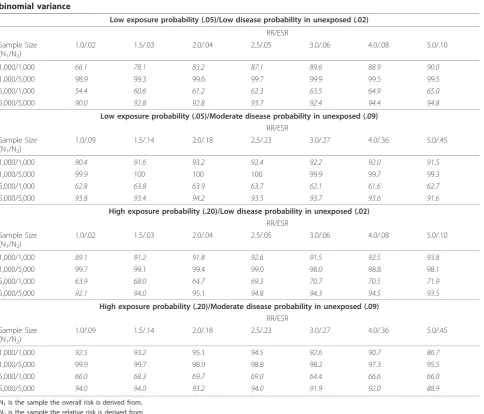
99% when the sample size the overall risk was derived Table 4 Coverage probability of the 95% confidence interval for the revised product-based estimator (ESRR) using a binomial variance

RR/ESR Sample Size

(N1/N2)

1.0/.02 1.5/.03 2.0/.04 2.5/.05 3.0/.06 4.0/.08 5.0/.10

1,000/1,000 66.1 78.1 83.2 87.1 89.6 88.9 90.0

1,000/5,000 98.9 99.3 99.6 99.7 99.9 99.5 99.5

5,000/1,000 54.4 60.6 61.2 62.3 63.5 64.9 65.0

5,000/5,000 90.0 92.8 92.8 93.7 92.4 94.4 94.8

Low exposure probability (.05)/Moderate disease probability in unexposed (.09) RR/ESR

Sample Size (N1/N2)

1.0/.09 1.5/.14 2.0/.18 2.5/.23 3.0/.27 4.0/.36 5.0/.45

1,000/1,000 90.4 91.6 93.2 92.4 92.2 92.0 91.5

1,000/5,000 99.9 100 100 100 99.9 99.7 99.3

5,000/1,000 62.8 63.8 63.9 63.7 62.1 61.6 62.7

5,000/5,000 93.8 93.4 94.2 93.5 93.7 93.6 91.6

High exposure probability (.20)/Low disease probability in unexposed (.02) RR/ESR

Sample Size (N1/N2)

1.0/.02 1.5/.03 2.0/.04 2.5/.05 3.0/.06 4.0/.08 5.0/.10

1,000/1,000 89.1 91.2 91.8 92.6 91.5 92.5 93.8

1,000/5,000 99.7 99.1 99.4 99.0 98.0 98.8 98.1

5,000/1,000 63.9 68.0 64.7 69.3 70.7 70.5 71.9

5,000/5,000 92.1 94.0 95.1 94.8 94.3 94.5 93.5

High exposure probability (.20)/Moderate disease probability in unexposed (.09) RR/ESR

Sample Size (N1/N2)

1.0/.09 1.5/.14 2.0/.18 2.5/.23 3.0/.27 4.0/.36 5.0/.45

1,000/1,000 92.5 93.2 95.1 94.5 92.6 90.7 86.7

1,000/5,000 99.9 99.7 98.9 98.8 98.2 97.3 95.5

5,000/1,000 66.0 68.3 69.7 69.0 64.4 66.6 66.0

5,000/5,000 94.0 94.0 93.2 94.0 91.9 92.0 88.9

(8)

from was 1,000 and the sample size the RR was derived from was 5,000 (Table 4).

The expected lengths given coverage for Scenario 3 is shown in Figure 3. Compared to Scenario 1 (Figure 1) and Scenario 2 (Figure 2), the expected lengths have decreased substantially. Also, as in Scenario 2, the expected lengths for all of the 95% CIs increased as the magnitude of the RR increased.

Scenario 4: High exposure probability (.20)/Moderate disease probability among unexposed (.09)

In Scenario 4 we increased both the exposure probabil-ity (.20) and the disease probabilprobabil-ity among the unex-posed (.09) at the same time. This gave similar results to Scenario 3. The observed relative bias of ESRS

increased with increasing RR, while the observed relative bias was near 0% for ESRR. Coverage probabilities for

the 95% CI of ESRS decreased substantially as the RR

increased. Coverage probabilities for the 95% CIs for ESRR using a log-based variance and binomial variance

were not affected by the magnitude of the RR. Expected lengths given coverage also showed similar relationships that were previously described (Figure 4).

In Scenario 4, we also evaluated the properties of our estimator when the sample size was 250 for both samples. We observed similar relationships in terms of observed relative bias and coverage probabilities. The observed rela-tive bias of ESRSwas 7.8% when the RR was 1.0 and 84.9%

when the RR was 5.0, while the observed relative bias of ESRRranged between -1.1% and 1.1%. The coverage

prob-ability of the 95% CI for ESRSwas 96.8% when the RR was

1.0 but fell below 95% when the RR was 1.5 (92.3%) and decreased substantially for a RR of 5.0 (56.8%). The cover-age probability of the 95% CI for ESRRusing a log-based

variance was greater than 95% for all RRs. The coverage probability of the 95% CI for ESRR using a binomial

Figure 1Expected length given coverage for 95% confidence intervals of the ESRS, ESRRusing a log-based variance, and ESRRusing a

(9)

variance ranged between 85.7 and 92.5%. In terms of expected length given coverage, the 95% CI for ESRRusing

a binomial variance provided shorter intervals and were closer to the length of the empirical interval than the 95% CI using a log-based variance.

Results of the case study

Results of the case study are shown in Table 5. The esti-mated risk of symptomatic knee OA was slightly higher when using the simple product-based method. The esti-mate of the risk of symptomatic knee OA in obese per-sons ranged between 0.57% and 2.11% when using the revised product-based method. All 95% confidence inter-vals overlapped with one another for each age group.

Discussion

We have shown via a simulation study that the simple product-based estimator (ESRS) that has been calculated

in previous studies only performs well in certain situa-tions. Mainly, those situations are when the exposure probability is low (~5%) and the magnitude of the RR is small (~3.0). There are two reasons for this and they can easily be seen by deconstructing the overall risk of disease using the law of total probability.

P(D)=P(D|E)*P(E)+P(D|E)*P(E) (13) Recall that for the product-based estimator of the ESR to be unbiased that what we really need is an estimate of the risk of disease in the unexposed and not the over-all risk. When the exposure probability is low, less weight is put on the probability of disease among the exposed. Put this together with a small RR and most of the overall risk of disease is being influenced by those who are unexposed. However, increasing the exposure probability puts more weight on the risk of disease

(10)

among the exposed, which will give you a much more biased estimate of the risk of disease among the unex-posed. We also showed that ESRRprovides a substantial

improvement over the ESRSin terms of observed

rela-tive bias. We found that the observed relarela-tive bias of ESRRwas near 0% in almost all cases.

Coverage probabilities for the 95% CI for ESRSwere

inversely related to the observed relative bias of ESRS. As

the observed relative bias increased, the coverage probabil-ity decreased. The overestimation of the ESR using exist-ing methodology (ESRS) led to 95% CIs that were less

likely to cover the true ESR. Also, the expected lengths given coverage for these 95% CIs were usually longer than the lengths produced for ESRRusing either the log-based

variance or the binomial variance rendering this method of point and interval estimation to be sub-optimal.

Coverage probabilities for the 95% CI for ESRRusing a

log-based variance exhibited greater than 95% coverage

in most cases. The exception was when the sample size for the overall risk was 1,000 and the sample size for the RR was 5,000. Paradoxically, this was the only situa-tion in which the 95% CI of ESRRusing a binomial

var-iance exhibited greater than 95% coverage. In terms of expected length given coverage, neither of these two methods of interval estimation of ESRRperformed better

than the other in all situations. The coverage probability and expected length given coverage depended on the variance estimate that was employed. From equation 11, we can see that the log-based variance of ESRR took

into account variability from the overall risk and the RR. We also assumed that the two measures were indepen-dent and had a covariance of zero, which is a reasonable assumption because the two measures come from two independent samples. From equation 12, we can see that the binomial variance of ESRRprobability of

expo-sure from sample 2 so that the variance would not be

(11)

under-estimated. However, in most cases the variability still was under-estimated. When the sample sizes were equal, the under-estimation was very little since the cov-erage probabilities ranged from 87%-95% in most cases.

However in Scenario 1, when the sample size combina-tion was 1,000/1,000 and the RR was 1.0, 1.5, and 2.0 the coverage probabilities were 66%, 78%, and 83% respectively.

binomial variance in Scenario 4. Empirical 95% confidence intervals are also shown. The analysis assumed an exposure probability of .20 and risk of disease in the unexposed of .09. The x-axis is the magnitude of the RR. Results are from simulations where both N1and N2are 5,000. Note: The expected length given coverage for the 95% CI around ESRScould not be computed when the RR was 5.0 because the coverage probability was 0.

Table 5 Results from the case study on the risk of symptomatic knee OA in obese persons

Age

Overall risk of symptomatic knee OA in the Oliveria

study

Risk of symptomatic knee OA for obese persons using the simple product-based method

95% CI for ESRSusing a

log-based variance

Risk of symptomatic knee OA for obese persons using the

revised product-based method

95% CI for ESRRusing a

log-based variance

95% CI for ESRRusing a

binomial variance

50-59

0.0040 0.0076 0.0052-0.0110 0.0057 0.0038-0.0085 0.0037-0.0077

60-69

0.0087 0.0167 0.0121-0.0230 0.0125 0.0089-0.0175 0.0095-0.0155

70-79

0.0147 0.0282 0.0207-0.0383 0.0211 0.0153-0.0289 0.0168-0.0253

*Probability of being obese was derived from the Niu study (0.371).

(12)

The four scenarios, which were defined by the combi-nations of two different exposure probabilities (.05 and .20) and two different probabilities of disease in the unexposed (.02 and .09), did not affect the observed relative bias of ESRR. However, as we increased these

two parameters, the observed relative bias of ESRS

increased. This phenomenon was also demonstrated when comparing coverage probabilities based on the log-based variance for ESRRand ESRS. When comparing

coverage probabilities based on the binomial variance for ESRR, the scenario does matter with larger values of

the probability of exposure and/or probability of disease in the unexposed increased coverage probabilities. This is not surprising because the estimate of the binomial variance will increase with increasing exposure probabil-ities and increasing probability of disease among the unexposed.

Results from our case study most closely resemble scenario two where the magnitude of the RR is 2.0. In scenario two, we assumed an exposure probability of 0.20 and a probability of disease in the unexposed of .02. In our case study the RR was 1.91, the exposure probability (probability of being obese) was 0.371, and the overall risk of disease (symptomatic knee OA) ran-ged from 0.0087 to 0.0132. While the simulations sug-gest that the estimator would be biased, the overall risk of disease is small so the difference between the two estimates in absolute terms is not large with the largest over-estimation occurring in those ages 70-79 by 0.71%.

It is likely that the estimates produced by Horsburgh and Stewart et al. were accurate. In the article by Hors-burgh et al on tuberculosis, he estimated the ESR of tuberculosis for those with advanced HIV infection; old, healed tuberculosis; and immunosuppressive therapy[1]. While the RR of obtaining a new case of tuberculosis is high for those with advanced HIV infection and old, healed tuberculosis, the probability of exposure is so low for these exposures that the impact of the large RR would be muted. For those with immunosuppressive therapy, the RR of a new case of tuberculosis is modest (2.0) and the probability of exposure is low so the over-all probability of disease is a good estimate of the prob-ability of disease among those who are not on immunosuppressive therapy [1]. In the Stewart article, the largest RR is 4.62, but this corresponds to an expo-sure probability of 0.001. When the expoexpo-sure probabil-ities are large enough to possibly impact the estimate of the ESR, the RR is low enough (< 2.0) to offset the pos-sible bias [2].

An article by Cupples et al. calculated risk curves for first-degree relatives of patients with Alzheimer’s dis-ease. Their method used the odds ratio instead of the

relative risk and included converting probabilities to odds [6]. Our method will allow clinicians and other researchers to find the ESR in one step, provided the summary statistics needed for the calculation (P1(D),

RR2, and P2(E)) are available.

We acknowledge that there are limitations with this study. The first is that simulation studies can not be considered a proof. However, we did show mathemati-cally that the proposed estimator of the ESR is unbiased and the results of our simulation confirm this finding. It would be important to show mathematically what the true coverage probabilities are for our 95% CIs across different RRs, exposure probabilities, and probabilities of disease among the unexposed. We also acknowledge that our simulations showed coverage probabilities that well exceed 95% when we are calculating 95% CIs for ESRRusing a log-based variance.

We also evaluated the properties of our point and interval estimators when the sample size was small. We observed that one should only consider carrying out these calculations in smaller samples if the prevalence of exposure and disease among the unexposed is suffi-ciently large. If one of these values is small than the validity of the estimate of the RR may be questionable. Thus, we recommend that investigators using this meth-odology only use estimates that are of the highest quality.

The implications of our study are substantial. Clini-cians can use these estimates to better explain risk of disease to patients. Many times clinicians and patients can misinterpret the meaning of having a certain RR of disease. Interpreting the probability of disease given a certain exposure (the ESR) is much more transparent. Future studies that examine the calculation of ESRs may look at the impact of having the odds ratio (OR) rather than the RR. Also, the consideration of under which study designs and magnitudes of the exposure/disease would an approximation using the OR be valid is an important question to answer. It is likely that the OR would be valid when the prevalence of the outcome is less than 10% but examining this rigorously would be of great importance [7]. Lastly, re-sampling and bootstrap-ping techniques may be a useful method of obtaining CIs with appropriate coverage.

Conclusions

(13)

Additional material

Additional file 1: Tables displaying results for absolute bias, relative bias, and coverage probabilities for all simulation scenarios. Results from all simulations.

List of abbreviations

ESR: Exposure specific risk; RR: Relative risk; CI: Confidence interval; D: Disease; D¯: Without disease; E: Exposure; E¯: Without exposure; P(): Probability of; Var: Variance; Cov: Covariance; exp(): exponential function; OA: osteoarthritis.

Acknowledgements

Grant support: This research was supported in part by the National Institutes of Health, National Institute of Arthritis and Musculoskeletal and Skin Diseases grants T32 AR055885 and K24 AR057827.

Author details

1_{Department of Orthopedic Surgery, Brigham and Women}_’_{s Hospital, 75}

Francis Street, Boston, MA 02115, USA.2_{Department of Biostatistics, Boston} University School of Public Health, 801 Massachusetts Avenue, Boston, MA 02118, USA.3_{Department of Epidemiology, Boston University School of} Public Health, 715 Albany Street, Boston, MA 02118, USA.4Massachusetts Veterans Epidemiology Research and Information Center, VA Cooperative Studies Program, Veterans Affairs Medical Center, 150 S. Huntington Ave, Jamaica Plain, MA 02130, USA.

Authors’contributions

WMR designed the simulation study, interpreted the data, wrote and critically revised the manuscript, and gave final approval of the manuscript. DG interpreted the data, critically revised the manuscript, and gave final approval of the manuscript. CRH interpreted the data, critically revised the manuscript, and gave final approval of the manuscript. EL designed the simulation study, interpreted the data, critically revised the manuscript, and gave final approval of the manuscript

Competing interests

The authors declare that they have no competing interests.

Received: 14 May 2010 Accepted: 5 January 2011 Published: 5 January 2011

References

1. Horsburgh CR Jr:Priorities for the treatment of latent tuberculosis infection in the United States.N Engl J Med2004,350(20):2060-2067. 2. Stewart A, Calder LD, Torgerson DJ, Seymour DG, Ritchie LD, Iglesias CP,

Reid DM:Prevalence of hip fracture risk factors in women aged 70 years and over.QJM2000,93(10):677-680.

3. Buehler RJ:Confidence Intervals for the Product of Two Binomial Parameters.J Am Stat Assoc1957,52:482-93.

4. Oliveria SA, Felson DT, Reed JI, Cirillo PA, Walker AM:Incidence of symptomatic hand, hip, and knee osteoarthritis among patients in a health maintenance organization.Arthritis Rheum1995,38(8):1134-1141. 5. Niu J, Zhang YQ, Torner J, Nevitt M, Lewis CE, Aliabadi P, Sack B, Clancy M,

Sharma L, Felson DT:Is obesity a risk factor for progressive radiographic knee osteoarthritis?Arthritis Rheum2009,61(3):329-335.

6. Cupples LA, Farrer LA, Sadovnick AD, Relkin N, Whitehouse P, Green RC: Estimating risk curves for first-degree relatives of patients with Alzheimer_’s disease: the REVEAL study.Genet Med2004,6(4):192-196. 7. Zhang J, Yu KF:What’s the relative risk? A method of correcting the

odds ratio in cohort studies of common outcomes.JAMA1998, 280(19):1690-1691.

Pre-publication history

The pre-publication history for this paper can be accessed here: http://www.biomedcentral.com/1471-2288/11/1/prepub

doi:10.1186/1471-2288-11-1

Cite this article as:Reichmannet al.:Evaluation of exposure-specific

risks from two independent samples: A simulation study.BMC Medical

Research Methodology201111:1.

Submit your next manuscript to BioMed Central and take full advantage of:

• Convenient online submission

• Thorough peer review

• No space constraints or color figure charges

• Immediate publication on acceptance