Influence of insertion of holes in the middle of obstacles on the flow around a surface-mounted cube

(1)

73 *_{Corresponding author}

Influence of insertion of holes in the middle of obstacles on the flow

around a surface-mounted cube

B. Rostanea, _{*, K. Aliane}a_{and S. Abboudi}b

a_{MECACOMP Laboratory, University of Tlemcen, FT, Department of Mechanics, BP 230, 13000 Tlemcen,} Algeria

b_Laboratoire_{Interdisciplinaire Carnot de Bourgogne-UTBM, CNRS and University of Bourgogne Franche} Comté (UBFC), Dijon, France

Article info: Abstract

The aim of this study is to analyze the impact of insertion holes in the middle of obstacles on the flow around a surface-mounted cube. Four configurations of obstacles in a channel with a Reynolds number, based on obstacle height, ReH =

40000 are studied. The hexahedral structured meshes are used to solve the fluid dynamics equations. The finite volume method is employed to solve the governing equations using the ANSYS CFX code and the turbulence model k-ω SST. The streamwise velocity profiles, time-averaged streamlines, turbulence kinetic energy, and drag coefficient are presented. The results show the appearance of a second vortex behind obstacles with the hole from diameter D/H=0.2. The turbulence kinetic energy is greater on top of the obstacle. It is more intense for the obstacle with no hole, as this intensity decreases with the increase in the hole diameter.The drag coefficient is improved only for the case D/H=0.32.

Received: 13/08/2018 Accepted: 25/02/2019 Online: 25/02/2019

Keywords:

Turbulent flow, Obstacle,

Surface-mounted cube, Obstacle with hole,

k-ω SST.

Nomenclature

CD Drag coefficient

D Hole diameter, [m]

h H

Channel height, [m] Height of obstacle, [m]

k Turbulent kinetic energy, [m²/s²]

L Channel width, [m]

pref Reference.pressure, [Pa]

Reh Reynolds number on the channel

height

ReH Reynolds number on the cube

height

Ub Mean bulk velocity, [m/s]

u 𝑢̅𝑖

u̅j

𝑢𝑖′𝑢𝑗′

̅̅̅̅̅̅

y+

ε

ρ µ µt ω

LDV LES

Velocity in x direction, [m/s] Time averaged.velocity in xi

direction, [m/s]

Time averaged.velocity in xj

direction, [m/s]

Turbulent stresse, [m²/s] Distance without dimensions Turbulent dissipation energy density, [kg/m3_]

Dynamic viscosity, [Pa.s] Turbulent.viscosity, [Pa.s] Specific dissipation, [1/s]

Subscripts

(2)

74

RANS

URANS

SST ANSYS CFX

Reynolds-averaged Navier– Stokes equations

Unsteady Reynolds-averaged Navier–Stokes equations Shear stress transport

Computational fluid dynamics software

1.

Introduction

The studies of flow around a bluff body represent references for researchers because they have a major contribution to understand the fundamental basics of building aerodynamics, such as the prediction of wake flow behind building structures,study of pollution around the urban area, and also improving the performance of air flat-plat solar thermal collector with baffle by understanding the internal aerodynamics of this type of flow to minimize the dynamic losses. Generally, the bluff body generates complex flow structures, including separation, reattachment, and vortical patterns. These flow structures are particularly complex because there is a phenomenon of turbulence.

The main experimental measurements for the wall mounted cube was developed by Martinuzzi and Tropea [1]. They examined the effects of the three-dimensional flow field around prismatic obstacles with different widths. They used various flow visualization techniques such as laser visualization, crystal violet, and oil film by static pressure measurements at Reynolds number of 40.000 based on the cube height, and presented the velocity profiles, streamlines, and pressure coefficient data.

Hussein and Martinuzzi [2] used a similar experiment with a different cubic obstacle. With the use of LDA (Doppler Anemometry Laser), they presented the rate of turbulence dissipation, production conditions, as well as the transport and equilibrium of the equation of transport of turbulent kinetic energy.

The experiment

helped to identify

different scales appropriate to the different flow characteristics around the cube (e.g., wake, boundary layer, and horseshoe vortex). Becker et al. [3] studied the case of a three-dimensional wind around a prismatic obstacle for a Reynolds number 20000≤Re≤70000. The addiction of the flow

structure with different angles of attack was examined. The results allowed to show a different topology of the "vortex arc" for different angles of attack. In the case of the tandem obstacles aligned in the direction of flow. Oke [4] studied the H / E and L / H, where

L and E respectively indicate the width of a building and Spacing between two buildings in the direction of flow. The experience showed the existence of three regimes, depending on the size of the buildings and the distance separating them, isolated obstacle flow, wake interference flow and skimming flow. Meinders and Hanjalic [5] studied the case of a tandem of staggered cubes for zero transverse and longitudinal spacings lower than 3H, where H is the height of the cubes. Presence of the downstream obstacle creates an asymmetry of the mean flow around two obstacles. Vortices structures around a surface-mounted pyramid were investigated by Mazen et al. [6] using Oil-film flow visualizations and LDV techniques for topology principles and velocity measurements. They found three pairs of vortices; a hairpin vortex behind the pyramid apex, a pair of vortex formed on opposite pyramid side face corners, and a pair of counter-rotating vortex formed vertically downstream of the obstacle. The study of the variation in Reynolds number in flow around a suspended cube was reported by Khan et al. [7]. The experiment was done on a very wide range of Reynolds number (500≤Re≤55000) whither authors showed that the stream was seen to be structureless at a greater Reynolds number and drag coefficients were

obtained

between 0.63 and 0.89.

Regarding the numerical approach, diverse

researchers

have considered the learning of the flux around bluff body experimentally using different turbulence models. Rodi [8] studied numerically the flow around a cubic obstacle of height H in a channel. The authors tested two versions of turbulence model of RANS and LES and compared them with the experimental results of Martinuzzi and Tropea [1] with a Reynolds number based on the height of the obstacle ReH = 40000. They found that the RANS

(3)

JCARME Influence of insertion of holes . . . Vol. 9, No. 1

75 another work, Iaccarino and Durbin [9] studied

numerically the flow around a cube, referring to the Hussain and Martinuzzi experiment. For the calculation, two approaches of the RANS

(steady) and URANS (unsteady) models were taken, and they used the v2-f turbulence model. The results revealed that the URANS solution (unsteady RANS) is more realistic than the RANS

solution, and gives low cost results compared to those of the LES. Aliane et al. [10] gave numerical testing of flow around two types of obstacles: a rectangular obstacle and a rectangular obstacle with an upstream rounded edge with a radius of curvature 0.2 times the height of the obstacle in the two-dimensional simulation. The impact of the curvature on the recirculation zones in three positions, relative to the obstacle and velocity profiles, were presented. Sari-hassoun et al. [11] arrived to decrease the wake zone behind the obstacle; they changed the form of the upstream edge. Rostane et al. [12] studied two types of obstacles; prismatic with the sharp edges and prismatic with the rounded downstream edge. The authors analyzed the aerodynamic phenomena as the incipient structure of vortices near the obstacles and the effect of the curvature of the downstream edge on the reattachment area for a Reynolds number Reh=105. In another context, some researchers [13 and 14] studied the flow around perforated elements using new models. Mousazadeha et al. [15] analyzed laminar convective heat transfer around two cubic obstacles placed in tandem and staggered rows. The test results demonstrate that the temperature distribution is highly reliant on the flow structure and the drag coefficient is higher in the tandem arrangement.

The contribution of the present study is to analyze the impact of insertion holes in the middle of obstacles in order to control the amplitude of the separation, reattachment length, and the

swirl

constitutions in the three-dimensional simulation. To perform this, the impact of three radii of hole: D/H=0.08, 0.20 and 0.32, where D is the diameter of the hole and H

is the height of the cube, is investigated. The simulation is made for a Reynolds number

ReH=4.104.

2. Problem statement

2.1. Geometrical models

The different models of obstacles used in this study

are surface-mounted cubes with and

without holes

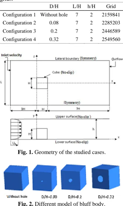
. The illustration of the problem is summarized in Fig. 1. The diameter of holes is varied between D/H=0.08, 0.2 and 0.32 (Fig. 2). Four configurations are employed (Table 1). The cube height is H=2.5 mm, and

the elevation of

the channel

is h=2H.

Table 1. Resume of the obstacle geometries and grids.

D/H L/H h/H Grid

Configuration 1 Without hole 7 2 2159841

Configuration 2 0.08 7 2 2285203

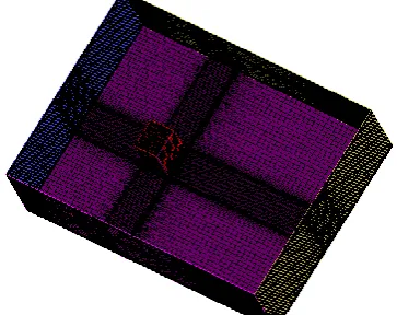
Fig. 1. Geometry of the studied cases.

Fig. 2. Different model of bluff body.

2.2. Mathematical model

(4)

76

𝜕𝑢̅𝑖

𝜕𝑥𝑖

= 0 (1)

𝜕𝑢̅𝑖

𝜕𝑡 + 𝑢̅𝑗 𝜕𝑢̅𝑖

𝜕𝑥𝑗

= −1 𝜌

𝜕𝑝̅ 𝜕𝑥𝑖

+ 𝜈𝜕

2_𝑢̅ 𝑖

𝜕𝑥𝑗2

−𝜕𝑢𝑖 ′_𝑢

𝑗′

̅̅̅̅̅

𝜕𝑥𝑗

(2)

For the treatment of turbulence, the model of Menter [16] k-ω SST (Shear Stress Transport) is used. This model combines two models: k-ω

model, proposed by Wilcox [17] for the area close to the wall, and the standard k-ε model, proposed by Jones and Launder [18], for the area far from the wall. Menter et al. [19] gave two equations for k and ω as follows:

𝐷(𝜌𝑘)

𝐷𝑡 = 𝑃̃𝑘− 𝛽

∗_{𝜌𝜔𝑘 +} 𝜕

𝜕𝑥𝑗

[(𝜇 + 𝜎𝑘𝜇𝑡)

𝜕𝑘 𝜕𝑥𝑗

] (3)

𝐷(𝜌𝜔) 𝐷𝑡 = 𝛼𝜌𝑆

2_{− 𝛽}∗_𝜌𝜔2₊ 𝜕

𝜕𝑥𝑗

[(𝜇 + 𝜎𝜔𝜇𝑡)

𝜕𝜔 𝜕𝑥𝑗

]

+ 2(1 − 𝐹1)𝜌𝜎𝜔2

1 𝜔 𝜕𝑘 𝜕𝑥𝑗 𝜕𝜔 𝜕𝑥𝑗 (4)

where 𝑃̃_𝑘_{is a production limiter}

_{for preventing}

accumulation of turbulence in stagnation areas as:

𝑃̃𝑘= 𝑚𝑖𝑛 [𝜇𝑡 𝜕𝑢𝑖 𝜕𝑥_𝑗(

𝜕𝑢̅_𝑖 𝜕𝑥_𝑗+

𝜕𝑢̅_𝑖 𝜕𝑥_𝑗, 10𝛽

∗_{𝜌𝜔𝑘)]}₍₅₎

and 𝐹1is a blending function as:

𝐹1= 𝑡𝑎𝑛ℎ ([𝑚𝑖𝑛 {

𝑚𝑎𝑥 ( √𝑘

𝛽∗_𝜔𝑦, 500𝜈 𝑦2_𝜔) , 4𝜌𝜎𝜔2𝑘 𝐶𝐷𝑘𝜔𝑦²

}]

4

) (6)

Here, y is the distance to the nearest wall. In the near-wall region, 𝐹1= 1, while it goes to zero in the outer region 𝐶𝐷𝑘𝜔as given bellow:

𝐶𝐷𝑘𝜔= 𝑚𝑎𝑥 (2𝜌𝜎𝜔2 1 𝜔

𝜕𝑘 𝜕𝑥_𝑗

𝜕𝜔 𝜕𝑥_𝑗, 10

−10₎₍₇₎

The constants of the model are:

𝐶𝜇= 0.09, 𝜎𝑘1= 0.85034, 𝜎𝑘2= 1, 𝜎𝜔1= 0.5,

𝜎𝜔2= 0.85616, 𝛼1= 0.5532, 𝛼2= 0.4403 ,

𝛽1= 0.075, 𝛽2= 0.0828, 𝛽∗= 0.09,

𝛼1= 0.31, 𝑐1= 10.

The k-ω SST model provides highly accurate predictions of the beginning and the amount of flow separation under adverse pressure gradients. It is recommended for high accuracy boundary layer simulations, so it is the ideal model for the present simulation.

2.3. Numerical approach

An unsteady 3D flow is used for these configurations, employing the ANSYS CFX-13 code. The size of the computational domain is

11H × L × 2H. The inlet of the computational field situated at an interval of 3H upstream of the cube, and the fully developed velocity profiles are used with the Reynolds number (Reh=Ubh/ν) equals 8.0×104_{. At the outlet of the system,}

constant pressure is maintained pout=pref. At the solid walls, no-slip conditions are imposed (upper surface, lower surface, and cube). The side boundaries are considered as slip surfaces, employing the symmetry conditions. The hexahedral structured meshes are used to solve the fluid dynamics equations (Fig. 3). The numbers of meshes are presented in Table 1. Turbulence model k-ω SST is used,so

the mesh

must be refined close to the

solid walls (y+<1). Integration on finite volume of the equations described above provides an ensemble of discrete equations. The numerical scheme upwind of second order is taken to discretize the convective terms. The velocity–pressure coupling is performed using a coupled solver to resolve the hydrodynamic equations (for u, v, w, p) as a single system (the method proposed by Rhie and Chow [20]).

(5)

JCARME Influence of insertion of holes . . . Vol. 9, No. 1

77 3. Results and discussion

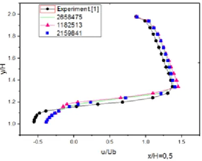
A preliminary study of the dependence of the calculation grid is carried out. Three grids comprising 1182513, 2159841 and 2658475

hexahedral elements are tested (Fig. 4). This study proves that there are relatively small differences between the three grids. The grid comprises 2159841 elements is the best compromise between precision and calculation time.

Fig. 4. Mesh sensitivity test.

In this simulation, the model of turbulence and the numerical method, used by studying the case of the configuration 1, are validated, and the results obtained from the simulation are compared to the experimental work of Martinuzzi and Tropea [1]. Fig. 5(a-c) depicts the velocity profiles in the flow direction in the area close to the obstacle for three separate sections of x/H=0.5, x/H=1, and x/H=1.5 for the Reynolds number Reh=105. The findings of the present simulation are almost coherent with those found experimentally by Martunizzi and Tropea [1].

The numerical predictions of the different vortex structures around the obstacle in the region close to the cube have been compared and validated by the experimental oeuvre of Hussein and Martinuzzi [2] for a Reynolds number

Reh=8,0×104_{(Fig. 6).}

A recirculation zone emerged upstream from the obstacle blocks by the leading face of the cube (zone A of the study conducted by Hussein and Martinuzzi [2] and zone A' of the present work).

Above the cube, the two figures (Fig. 6(a) and (b)) show the detachment point in the leading edge of the cube (points C and C'). The two figures also show the recirculation region downhill of the obstacle and indicate a very great resemblance (zones B and B').

Fig.5. Velocity curves in the plane z/H=0 at the positions of(a) x/H=0.5, (b) x/H=1, and (c) x/H=1.5.

(a)

(b)

(6)

78

Fig. 6. Streamlines on plane z/H=0;(Reh=8,0 × 104);

(a) Exp. [2] (see Ref. [21]), and (b) k −ωSST.

Table 2 gives the numerical predictions of separation and reattachment length of the flow. The comparison of the present results with those reported by other authors shows good agreement.

Table 2. Lengths for reattachment: XR/H, and

separation:XS/H.

Figs. 7-10 show the perspective views of flow field and vortices for the four studied cases; horseshoe vortex (D), side vortex (E), arc-shaped vortex (F), separation (G), and reattachment (H) points can be seen.

Fig. 7. 3D streamlines (cube without hole).

Fig. 8. 3D streamlines (D/H=0.08).

Fig. 9. 3D streamlines (D/H=0.2).

Fig. 10. 3D streamlines (D/H=0.32).

Contribution Model XR /H XS/H

Martinuzzi and

Tropea [1] Experiments 1.040 1.612

Rodi [8] LES 0.998 1.432

RANS 0.950 2.731

Shah [22] LES 1.080 1.690

Iaccarino and Durbin [9]

RANS Steady 0.640 3.315

RANS Unsteady 0.732 1.876

Breuer et al. [23] LES

(Smagorinsky) 1.287 1.696

Yakhot et al. [24] DNS 1.21 1.5

Present work k-ω SST 0.874 1.678

F

D G

E

H

(a)

(7)

79 Fig. 11. 2D streamlines in z/H=0 plane (cube without

hole).

Fig. 12. 2D streamlines in z/H=0 plane (D/H=0.08).

Table 3. Lengths for reattachment: XR/H, and

separation: XS/H for various studied cases.

case Without hole D/H=0.08 D/H=0.2 D/H=0.32

XR/H 1.678 1.87 1.94 1.71

XS/H 0.874 0.967 0.978 0.97

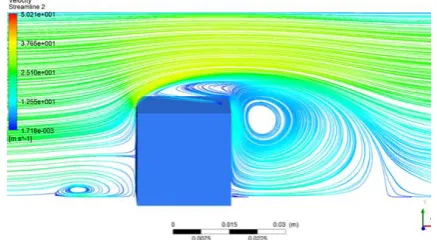
Figs. 11-14 depict streamlines at the symmetry plane of the channel for the four configurations. For the case of the cube without hole (Fig. 11), there is the appearance of three vortex regions: upstream and above and downstream of the cube. In the case of the obstacle with a hole of diameter D/H=0.08 (Fig. 12), the center of the vortex behind of the cube shifts to the right due to the jet coming out of the orifice. With the increase in the diameter of the orifice (Fig. 13)

(D/H=0.2), the jet deflects the downstream vortex downwards, allowing the vortex, above the obstacle, to lean down. Also, the appearance of another swirl is observed just above the jet,

and this may be due to the blocking the

swirling detachment in this area

. For the case of the obstacle with a hole of diameter equals 8 mm (Fig. 14), the downstream vortex is still leaning downwards by the force of the jet with increasing the size of the new vortex and the intensification of the vortex which is above the obstacle with a shift to the right.

Table 3 shows the values of the separation length

XS/H and reattachment XR/H of the fluid respect to the obstacle. It is noticed that the reattachment length increases by adding the hole because of the impact of the jet on the wake which is downstream of the obstacle (pushing it), and it is greater for the case D/H=0.2. Also, it is noted that the length of reattachment XR/H for the case

D/H=0.32 is lower than that of cases D/H=0.2

and D/H=0.08 due to the stronger jet, this jet presses the downstream vortex down.

The visualization of the various swirl forms indicated above gives a qualitative vision of the evolution of flow in the canal on each side of every obstacle model.

Then, it is necessary to

make a quantitative study which is

characterized by the velocity profiles to

define the problem under investigation.

The

velocity profiles in the flow direction are

carried out for three different positions in the

symmetry plane for different locations of

(8)

80

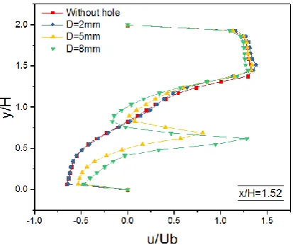
x/H=1.52 (Fig. 17). The distance y/H is taken between 0≤y/H≤2 for the first and third positions and 1≤ y/H≤2 for the second position.

According to Figs. 15 and 16, the velocity curves in the x direction are almost identical for the four cases with the presence of negative velocities which is due to the presence of the recirculation region upstream and on top of the obstacle. Fig. 17 can be divided into two parts: above

y/H=0.75, in which the velocity profiles are almost identical, and between 0 and 0.75, in which the velocity profiles of the cases of a cube with no hole and the cube with D/H=0.08 are identical. However, for the other cases, they have larger profiles due to the presence of the second vortex and jet.

Fig. 15. Velocity curves in x direction on the plane

z/H=0 at x/H =-0.68.

Fig. 16. Velocity curves in x direction on the plane

z/H=0 at x/H =0.5.

Fig. 17 . Velocity curves in x direction on the plane

z/H=0 at x/H=1.52.

The results of turbulence kinetic energy are presented in Figs. 18-21. The energy is higher on top of the obstacle, it is more intense for the obstacle without hole. The intensity decreases as the hole diameter increases (94.97 m²/s² for the obstacle without hole, 91.46 m²/s² for the obstacle with a hole D/H=0.08, 85.56 m²/s² for the obstacle with a hole D/H=0.2, and 86.09 m²/s² for the obstacle with a hole D/H=0.32). It is noted that the turbulence kinetic energy increases at the level of the jet (the exit of the hole).

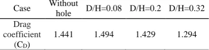
Investigating the fluid behavior from the viewpoint of dynamic on the models of obstacles is translated by the study of two resistances: the wall strength due to the viscous force and the resistance form of the obstacle. Both insert the notion of drag coefficient. Table 4 gives the drag coefficients for various treated cases.

It is noted that the drag coefficient is constant for the three configurations (without hole,

D/H=0.08 and D/H=0.29), except for the

(9)

81 Fig. 18. 2D contour of turbulence kinetic energy in

z/H=0 plane (without hole).

Fig. 19. 2D contour of turbulence kinetic energy in

z/H=0 plane (D/H=0.08).

z/H=0 plane (D/H=0.2).

z/H=0 plane (D/H=0.32).

Table 4. Drag coefficients obtained for all the geometries studied

Case Without

hole D/H=0.08 D/H=0.2 D/H=0.32

Drag coefficient

(CD)

1.441 1.494 1.429 1.294

4. Conclusions

In this work, a three-dimensional study of

turbulent flow around a bluff body is conducted to analyze the effect of hole insertion, founded on the URANS approach and employing the

ANSYS-CFX 13 code. The k-ω SST turbulence model is chosen to resolve the averaged Navier-Stokes equations. The model of turbulence and the numerical method are validated by studying the case of the obstacle with no hole, and the results obtained from the simulation are compared to the experimental works available in the literature.

Flow velocity profiles were validated for Reynolds number Reh = 8.0 × 104and 105 in the zone near the bluff body. The findings of the simulation used in the present study are almost coherent with those experimentally found and reported in the literature.

The figures of the streamlines show the structure of the nascent vortices around each type of obstacle, and there is vortex formation upstream, above and downstream of the cube. There is also the appearance of another swirl downstream of the cube above the jet for obstacle models with a hole having a diameter of D/H=0.2.

The reattachment length increases by adding the hole. For the streamwise velocity profiles, there is no significant change in upstream and on the top of the obstacle, but in downstream, the values of velocity increases with the increase in the diameter of the holes.

The turbulence kinetic energy is higher on the top of the obstacle; it is more intense for the obstacle with no hole, and the intensity decreases as the hole diameter increases.

Concerning the pressure loss, this study shows that only the cube with a hole, having a diameter of D/H=0.32 ensures an about 10%

improvement. References

[1] R. Martinuzzi, C. Tropea, "The flow around a surface-mounted prismatic obstacle placed in a fully developed channel flow", J. Fluids Eng, Vol. 115, No. 1, pp .85-92, (1993).

[2] H. J. Hussein, R. J. Martinuzzi, "Energy balance for the turbulent flow around a surface mounted cube placed in a channel",

Phys. Fluids, Vol. 8, No. 3, pp. 764-780, (1996).

(10)

82

boundary layers", Journal of Wind Engineering and Industrial Aerodynamics, Vol. 90, No. 4-5, pp. 265-279, (2002). [4] T. R. Oke, "Street design and urban canopy

layer climate". Energy and Buildings, Vol. 11, No.1-3, pp. 103-113, (1988).

[5] E. R. Meinders, K. Hanjalic, "Experimental study of the convective heat transfer from in-line and staggered configurations of two wall-mounted cubes". Int. J. Heat Mass Trans., Vol.45, No. 3 pp.465-482, (2002). [6] M. Mazen, R.J. Martinuzzi, "Vortical structures around a surface-mounted pyramid in a thin boundary layer" , Journal of wind engineering and industrial aerodynamics, Vol. 96, No. 6-7, pp. 769-778,(2008).

[7] M. H. Khan, P. Sooraj, A. Sharma, A. Agrawal, "Flow around a cube for Reynolds numbers between 500 and 55,000" Experimental Thermal and Fluid Science,Vol.93, pp. 257-271,(2018). [8] W. Rodi, "Comparison of LES and RANS

Calculation of the flow around bluff bodies", Journal of Wind Engineering and Industrial Aerodynamics", Vol. 69-71, pp. 55-75, (1997).

[9] G. Iaccarino, P. Durbin, "Unsteady 3D RANS simulations using the v2-f model",

Annual Research Briefs, Center for Turbulence Research, Stanford Univ., Stanford, CA, 2000, pp. 263–269, (1997). [10] K. Aliane, "Passive control of the turbulent

flow over a surface-mounted rectangular block obstacle and a rounded rectangular obstacle", International. Review of Mechanical. Engineering, Vol. 5, No. 2, pp. 305-314, (2011).

[11] Z. Sari-hassoun, K. Aliane, O. Sebbane, "Numerical simulation.study of the.structure of the separated flow around obstacles: curved edge effect",

International Journal on Heat and Mass Transfer - Theory and Applications", Vol. 1, No. 5, pp.276-284 (2013).

[12] B. Rostane, K. Aliane, S. Abboudi, "Three dimensional.simulation for turbulent.flow Around Prismatic Obstacle with. Rounded downstream edge using the k-ω SST

model", International Review of.

Mechanical. Engineering. Vol. 9, No. 3, pp.266-277, (2015).

[13] M. Dehghan, Y. Rahmani, D. D. Ganji, S. Saedodin,M. S. Valipour, S. Rashidi , "Convection- radiation heat transfer in solar heat exchangers filled with a porous medium: Homotopy perturbation method versus numerical analysis" Renewable Energy, Vol. 74, pp. 448-455, (2015). [14] M. Barzegar Gerdroodbary, D. D. Ganji,

Y. Amini "Numerical study of shock wave interaction on transverse jets through multiport injector arrays in supersonic crossflow" ActaAstronautica, Vol. 115, pp. 422-433,(2015).

[15] S. M. Mousazadeh, M. M. Shahmardan, T. Tavangar, Kh. Hosseinzadeh, D. D. Ganji, "Numerical investigation on convective heat transfer over two heated wall-mounted cubes in tandem and staggered arrangement" Theoretical and Applied.

Mechanics Letters, Vol. 8, No. 3, pp. 171-183, (2018).

[16] F. Menter, "Two-equation eddy-viscosity. turbulence models for engineering application", AIAA Journal, Vol. 32,No. 8, pp. 1598-1605, (1994).

[17] D. C. Wilcox, Turbulence Modeling for CFD Second Edition, D.C.W. Industries, (1998).

[18] W. Jones and B. Launder, "The calculation of low-Reynolds-number phenomena with a two-equation model of turbulence",

International Journal of Heat and Mass Transfer, Vol. 16, No. 6, pp. 1119-1130, (1973).

[19] F. Menter, M. Kuntz, and R. Langtry, "Ten years of industrial experience with the. SST turbulencemodel turbulence", Heat and Mass Transfer 4, Begell House, Inc, (2003).

[20] C. M. Rhie, W. L. A Chow, "Numerical Study of the Turbulent Flow Past an Isolated Airfoil with Trailing Edge Separation", AIAA journal, Vol. 21, No. 11, pp. 1525-1532. (1983).

[21] D. Lakehal, W. Rodi,"Calculation of the flow past a surface mounted cube with two-layer turbulence models". Journal of Wind.

(11)

83

Aerodynamics, Vol. 67 and 68, pp. 65-78, (1997).

[22] K. B. Shah, Large-eddy simulation of the flow past a cubic obstacle, PhD. Thesis, Stanford University, (1998).

[23] W. Rodi, J. H. Ferziger, M. Breuer, and M. Pourquié. "Workshop on LES of flows past

bluff bodies". Rotach-Egern, Germany,

(1995).

[24] A. Yakhot, H. Liu, N. Nikitin, "Turbulent flow around a wall-mounted cube: A direct numerical simulation". International Journal. of. Heat and Fluid. Flow, Vol. 27, No. 6, pp. 994-1009, (2006).