Xion, Y., Ge, Y., Liang, Y. and Blackmore, S. 2017. Development of a prototype robot and fast path‐ planning algorithm for static laser weeding. Computers and Electronics in Agriculture, 142 Part B,
Development of a prototype robot
and fast path-planning algorithm for
static laser weeding
by Xion, Y., Ge, Y., Liang, Y. and Blackmore, S.
Copyright, Publisher and Additional Information: This is the author accepted manuscript.
The final published version (version of record) is available online via Elsevier.
This version is made available under the CC-BY-ND-NC licence: https://creativecommons.org/licenses/by-nc-nd/4.0/legalcode
Please refer to any applicable terms of use of the publisher
DOI: https://doi.org/10.1016/j.compag.2017.11.023
Development of a prototype robot and fast path-planning algorithm
for static laser weeding
Ya Xiong
a, Yuanyue Ge
a, Yunlin Liang
a, Simon Blackmore
a,*a Engineering department, Harper Adams University, Newport, Shropshire, TF10 8NB, United Kingdom
Abstract
To demonstrate the feasibility and improve the implementation of laser weeding, a prototype robot was built and equipped with machine vision and gimbal mounted laser pointers. The robot consisted of a mobile platform modified from a small commercial quad bike, a camera to detect the crop and weeds and two steerable gimbals controlling the laser pointers. Visible class one laser pointers were used to simulate the power laser trajectories. A colour segmentation algorithm was utilised to extract plants from the soil background, size estimation was used to differentiate crop from weeds and an eroding and dilating algorithm was developed for objects that were touching. Conversely, another algorithm, which relied on shape descriptors, was able to distinguish plant species in non-touching status regardless of area difference. To reduce route length and run time, a new path-planning algorithm for static weeding was proposed and tested. It was demonstrated to be more temporally efficient especially when addressing higher density of weeds. A model to determine the optimal segmentation size based on time taken for treatment was established. It was found that the segmentation algorithm has the potential to be widely used in fast path-planning for the travelling-salesman problem. Finally, performance tests showed that the weeding mean error was 1.97 mm, with a 0.88 mm standard deviation. Another test indicated that with a laser traversal speed of 30 mm/s and a dwell time of 0.64 s per weed, it had a hit rate of 97%.
Keywords: Laser weeding robot; Fast path-planning; Machine vision; Dual-gimbal; Static weeding
1. Introduction
Weeds affect crop yield due to competition with the crops to acquire plant nutrients and resources (Slaughter et al., 2008). Currently, chemical weeding (herbicide) is widely used as a traditional weeding solution (Bakker et al., 2010). However, herbicides are viewed critically about their negative environmental impacts (Marx et al., 2012). Moreover, people increasingly require and prefer natural, organic foods (Blasco et al., 2002). There are also an increasing number of herbicide resistant weed species being recognised. (251 by International Survey of Herbicide Resistant Weeds). Many non-chemical weeding methods have been developed ranging from electrocuting [M.F. Diprose, F.A. Benson, Electrical methods of killing plants, Journal of Agricultural Engineering Research, Volume 30, 1984, Pages 197-209, ISSN 0021-8634, http://dx.doi.org/10.1016/S0021-8634(84)80021-9.
(http://www.sciencedirect.com/science/article/pii/S0021863484800219)] through to using mechanical or physical methods [Euro Pannacci, Boris Lattanzi, Francesco Tei, Non-chemical weed management strategies in minor crops: A review, Crop Protection, Volume 96, June 2017, Pages 44-58, ISSN 0261-2194, http://doi.org/10.1016/j.cropro.2017.01.012.
(http://www.sciencedirect.com/science/article/pii/S0261219417300212)]. Nørremark et al developed
cycloid weeding hoe for both inter and intra row weeds based in GPS position of the crop. [M. Nørremark, H.W. Griepentrog, J. Nielsen, H.T. Søgaard, The development and assessment of the accuracy of an autonomous GPS-based system for intra-row mechanical weed control in row crops, Biosystems Engineering, Volume 101, Issue 4, December 2008, Pages 396-410, ISSN 1537-5110, http://doi.org/10.1016/j.biosystemseng.2008.09.007.
(http://www.sciencedirect.com/science/article/pii/S153751100800278X)]. Tillett et al. (2008) developed a vision based inter and intra-row mechanical weeding robot using rotating discs for transplanted crops that can remove 80% of weeds. Similarly, Ahmad (2012) presented a rotating tine weeding mechanism for intra-row weeding robot. Besides, O’Dogherty et al. (2007) proposed a mathematical model for inter and intra-row hoeing. Moreover, another kind of mechanical weeding robot equipped with a real-time kinematics GPS to detect crop planting geopositions has been developed by Pérez-Ruiz et al. (2012). They reported the system has a mean error of 0.8 cm and 1.75 cm standard deviation when travelling at a speed of 0.8 km/h.
However, all of the above inter and intra-row mechanical weeding robots needed the crops to be well distributed. Selective weeding could provide solutions for crops regardless of distribution, which is more close to how human kill weed. In addition, it was reported that a selective weeding strategy could decrease the energy input even more by 10 to 90 % (Griepentrog et al., 2006). Midtiby et al. (2011) developed a real-time machine vision based micro-spraying weed control system, but only 37% of the smaller scentless mayweed were effectively controlled. After that, Underwood et al. (2015) presented a micro-dot targeted and steerable spraying robot for weeding control. However, selective spraying still relies on herbicides application, which is not allowed for organic farming. Due to the unsatisfactory aspects, other weeding techniques such as laser weeding seems to offer a potential alternative (Marx et al., 2012). Some researchers, such as Heisel et al. (2001), used a laser beam to cut weed stems for weed control. Another laser weeding application is to use laser irradiation. Marx et al. (2012) proposed a weed damage model for laser irradiation based weed control. Mathiassen et al. (2006) investigated the effects of laser treatment towards weeding. The results indicated that laser exposure time and laser spot size could be optimised to kill the weeds. Nadimi et al. (2009) designed a laser weeding test setup for simulate dynamic targeting weeding. However, none of the above researcher have successfully designed a whole mobile robot for the purpose of laser weeding.
Therefore, the aim of this study was to design and test in the laboratory a novel prototype laser weeding robot and explore its possibility and feasibility.
2. Materialsandmethods
2.1 System overview
Fig. 1. The laser weeding robot.
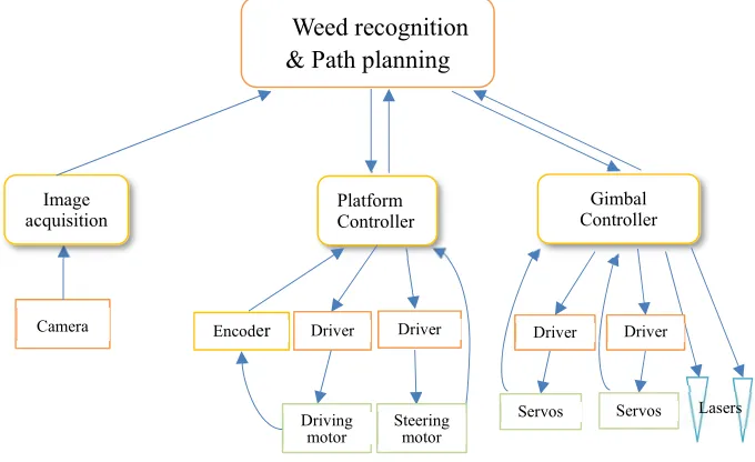
The system architecture is shown in Fig. 2. The three subsystems were coordinated by a central program written in MATLAB (2015a). The architecture used a distributed control strategy in such a way that each subsystem had an independent controller, which made the system easily integrated. The image acquisition grabbed the image and passed it to the weed recognition program. The weed centroids and path planning methods were then used to control the gimbals. Feedback loops were built into all levels of the Platform and Gimbal controllers.
Fig. 2. System architecture.
2.2 Platform controller
2.2.1 Robothardware
As shown in Fig. 1, the robotic platform had been modified from a small all-terrain vehicle (ATV) which was robotised by automating the steering and speed.
In terms of driving system control, the ATV itself had a motor driver that used a three-wire hall-effect
Driver Encoder
Platform Controller
Driver
Driving
motor Steeringmotor Camera
Image acquisition
Weed recognition & Path planning
Gimbal Controller
Driver Driver
speed control throttle to change the motor speed. The throttle was removed and it was found that it utilised 1-4 V analogue voltage to control vehicle speed, which could be provided by a PWM output of a microcontroller. Hence, an Arduino Mega 2560 was selected as the platform controller.
To achieve accurate and automatic steering control, as shown in Fig. 3, a Linak LA12.1P-100-12-01 linear actuator was used to rotate the steering mechanism. When the linear motor extended or retracted, the vehicle turned right or left accordingly and gave positional feedback to the controller. Both the maximum thrust and holding force of this actuator were 500 N, and therefore it could keep the steering angle stable regardless of normal moving resistance.
Fig. 3.Steering system: (a) extending-retracting linkage mechanism; (b) diagram of steering system; (c) linear actuator mounting.
2.2.2 Circuitdesignandcontrol
Two relays were used for the linear actuator control that provided three different states; extend, retract and hold. The relays were also controlled by the same Arduino as the driving system. The linear motor itself had a slide potentiometer so that it could send the stroke length as feedback.
The objective of the speed control was to achieve automatic speed adjustment, that matched the weed density. An optical encoder was mounted on the rear wheel for sensing platform displacement and speed. The platform was tested and the average time for moving the length of the tray (214 mm) was 1.56 s giving a maximum speed of 0.14 m/s.
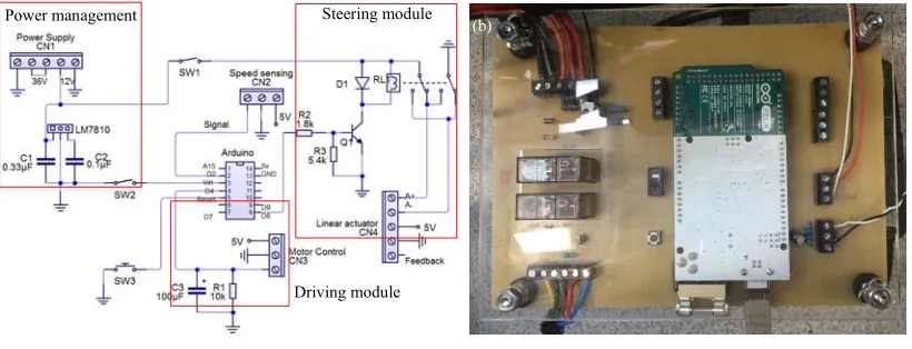
The vehicle controller interface was divided into three modules, power management, steering, and speed, as shown in Fig. 4.
Fig. 4.Main circuit of platform subsystem: (a) main circuit board schematic; (b) main circuit board. Power management
Driving module Steering module
(a) (b) (c)
2.3 Machine vision
2.3.1 Imageacquisitionandcoordinatetransformation
Burgos-Artizzu et al. (2011) proposed a one camera system for weed detection with pre-set height and camera angle. Similarly, this study used one camera with two preconditions, a fixed distance, and parallel to the ground, so that the coordinates of objects could be calculated. This method has some limitations such as it can only be used on a flat ground. However, the high image processing speed and simplicity of the system are also important aspects of this real-time weeding robotic system.
The camera model used was a GIGE DMK 23G618 from Sony, resolution 640x480, capturing speed 120 f/s. Images were imported to the weed recognition module via an Ethernet bus and processed. (“Computer Vision System Toolbox” from MATLAB). The camera was calibrated at first so that pixel coordinates of centroids could be transformed to real world coordinates. Based on classic Zhengyou Zhang calibration theory (Zhang, 2000), the camera was fixed while a chessboard had different poses for getting 15 calibration photos, which was used for obtaining camera intrinsic parameters and distortion coefficients.
2.3.2 Imageprocessingandweedrecognition
Image processing was divided into two steps. The first step was extraction of crops and weeds from the background, which was intent on obtaining a binary image that the crops and weeds were set as white pixels (1) while background was black (0). Based on the colour difference, this paper employed an algorithm that compared HSV (Hue, Saturation, and Value) of every pixel with pre-set colour thresholds to distinguish plants and background. However, because of changes in environment and light intensity, fixed HSV thresholds were not robust enough, so a colour-training algorithm was adopted. This method selected five different points on the plants and saved their HSV values. Then it set the tolerances (±0.1 in this paper) to all of the HSV values and therefore, it was employed to detect plants and background in other acquired images. Fig. 5(b) shows the extraction result of this method, in which big green leaves (regarded as crop) and clover (weeds) were extracted from grey soil and black tray. Since there were a lot of visual noise in the soil, the image was filtered by a medium filter afterwards. Then due to light influence, some holes could be found on plants, which influenced centroids calculation. Therefore, holes were filled by using “imfill” statement. The result, after using the above two processes, is demonstrated in Fig. 5(c). Additionally, the processing time of this method for Fig. 5(a) was 0.12 s.
(a) (b) (c)
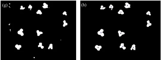
Fig. 5.Image processing protocol: (a) original photo; (b) using colour training to extract green plants from the background and get the binary image; (c) then filtering noise and filling holes of (b); (d) eroding of (c) until weeds disappeared; (e) dilating of (d) with a bigger value of erosion; (f) image (e) multiplied with (c) so that original shapes of crops were restored excluding small touching pars; (g) image (c) subtracted (f) to remove crops; (h) removed small objects and calculated centroids of weeds.
The second step was segmentation of weeds and crops so that weeds can be identified. Three segmentation methods were proposed, tested and compared. The first two segmentation algorithms assumed that weeds and crops had obvious area difference. The first one was based on area difference directly. The area was calculated in MATLAB by “regionprops” function and compared with a threshold to define if it was a weed or crop. However, there were always such situations that the weeds and crops were connected. Commonly used segmentation methods for touching objects, for example of “watershed”, are easy to split leaves of some species of weeds or crops, such as clover and dicotyledon, because their leaves are non-compact distributed, which are in a similar situation of touching between different plants. Therefore, the second method based on eroding and dilating had been implemented. In this method, Fig. 5(c) was eroded until all of the weeds disappeared, as shown in Fig. 5(d). Then dilating on Fig. 5(d) with a bigger value of erosion obtained Fig. 5(e), so the dilated figure contained entire crops. Next, Fig. 5(e) multiplied with Fig. 5(c), so that original shapes of crops were restored excluding some small touching parts, as seen in Fig. 5(f). After that, an important operation of subtracting Fig. 5(f) from Fig. 5(c) was performed to remove crops, as demonstrated in Fig. 5(g). Finally, Fig. 5(h) indicated the segmentation results after removing small objects and plotting centroids of weeds.
The processing time of the two algorithms for Fig. 5 by our equipment were 0.0958 s (based on area) and 0.0251 s (based on eroding and dilating), respectively. Therefore, “eroding and dilating” was much quicker and more effective.
Another segmentation method was based on shape features. Iivarinen et al. (1997) indicated that a combination of different shape descriptors was effective in object detection and needed less computation time, which is suitable for real-time system requirements. This team applied this method to plant detection. A combination of two shape descriptors, solidity, and compactness, was adopted. Solidity is object area divided by its convex area (implemented from the “regionprops” function in MATLAB). Compactness is a parameter to show how circular a shape is. It was defined as:
/ 4 ∗
Fig. 6 shows the processing results of classification based on shape descriptors. As shown in Fig. 6(a), there were two types of plants with similar area, a dicotyledon and a clover, respectively. Based on the above formula, Fig. 6(b) shows the comparison results of solidity and compactness between dicotyledon and clover. It is clear that both compactness and solidity of dicotyledons and clovers were obviously different, especially for compactness that clover was 0.394 bigger than dicotyledon in average. The final segmentation result can be seen in Fig. 6(c) where centroids of clovers were labelled. Also, the processing time of Fig. 6(a) was 0.063 s. In general, shape descriptors were easy and fast to distinguish plants regardless of area difference.However, it did not work in situation that plants were connected,
which is still a problem that needs to be solved.
Fig. 6. Processing results of the algorithm based on shape descriptors: (a) original picture; (b) solidity and compactness results of dicotyledon and clover; it is clear that compactness of clovers was bigger than dicotyledons while solidity of dicotyledons was higher than clover. (c) Segmentation results, centroids of clovers were labelled.
2.4 Dual-gimbal laser pointers
2.4.1 Gimbalspecificationandlasergroundresolutioncalculation
Blasco et al. (2002) designed a 6 DOFs (degrees of freedom) parallel robotic arm for mechanical weeding. Similarly, Underwood et al. (2015) used a Universal Robot 6 DOFs robotic arm for selective precision spraying and mechanical hoe weeding. These arms were utilized for contact weeding robot, which is complex and expensive. As for non-contact laser weeding robot, a 2 DOFs arm is enough. Two main requirements for gimbals are high speed and high precision. To increase weeding speed, as shown in Fig. 7(a), two gimbals were adopted, and they could work in parallel.
Fig. 7.Dual-gimbal and assembly schematic: (a) dual-gimbal; (b) assembly schematic of designed 2 DOFs arm.
Each gimbal assembly was made up of two Dynamixel servos, model MX-64. The rated resolution (∆) and no-load rotation speed were 0.088° and 378°/s, respectively. For security concerns, this prototype robot used two 5 V class 1 laser pointers to simulate the class 4 lasers needed to kill weeds. As shown in Fig. 7(b), two servos were mounted together by a 90° 3d-printed frame. The first servo ( ) was connected to the base and became the waist, while the second servo ( ), mounted in line with the ( ) rotational axis, became the shoulder. The laser pointer was mounted on the end of the second servo. Hence, the y coordinate (to the left) and the x coordinate (forwards) were determined by rotation angle of ( ) and ( ) respectively. In addition, the laser pointed on the ground, had a spatial uncertainty that was generated by both servos. The ground uncertainty area was non-uniformly distributed, and it varied from position to position. Assuming the target position of the laser point on the ground is , , 0 :
0.6 0.7 0.8 0.9 1
1 2 3 4 5 6
Sol
idity
Plant comparison number 0.5
0.8 1.1 1.4 1.72
1 2 3 4 5 6
C
om
pac
tn
es
s
Gimbal 1
Gimbal 2 Servo1
Servo2
Laser
Ground resolution area
·
Dicotyledon·
Clover(a) (b) (c)
∈ tan ∆ ∆ , tan ∆ ∆ 1
∈ tan ∆ ∆ , tan ∆ ∆ 1 eqn1.
Where “h” is the height of laser rotation centre above the ground. (320 mm for this test). The machine vision subsystem sent the real-world coordinates of weed centroids to the gimbal controller. Based on the above formulae, centroids could be converted into servo angles. As for laser ground resolution, it can be seen that the bigger the θ or α, the bigger the uncertainty range of x and y. Therefore, it was better to place the laser rotation centre on the top of the coverage area. In this paper, the coverage area for single gimbal was 200 mm (x direction) × 300 mm (y direction), so laser ground resolution (∆x, ∆y)
varied from (0.49 mm, 0.49 mm) to (0.54 mm, 0.60 mm).
2.4.2 Controlstrategy
The control diagram for the gimbals is shown in figure 8. Four servos and two lasers were directly controlled by an Arduino. MATLAB sent the target coordinates to the gimbal controller which then converted them into instruction packets and sent them to the servos. Each servo used its own built-in controller to give positional output. The servos also returned their positional status to the gimbal controller to compare the target position and the current position in real-time. The laser would be switched on when current position was approaching target position. Once the exposure time was reached, the laser would be turned off, and the gimbal controller sent back this information to MATLAB so that it could release the next position to gimbal subsystem for a new cycle.
Fig. 8.Schematic of gimbal control.
3. Weedingstrategiesandtesting
Two weeding methods were evaluated: static weeding and dynamic weeding. Static weeding meant that the platform stopped and carried out the laser operation and then moved on, while dynamic weeding, the robot kept moving and carried out weeding simultaneously. This paper reports the work on static weeding.
2.1 Path-planning algorithms
In static weeding, the robot firstly obtained all of the target locations in a single image frame, 640 × 480 pixels. Then the locations were sorted for weeding sequence. Sorting methods affected gimbal travelling route and processing speed. This is a TSP (travelling sales man) path-planning problem. Applegate et al. (2006) reported they used Concorde TSP Solver (try all trajectories) to process 85,900 points taking over 136 CPU years. This method could find out the best trajectory, but it was too
Laser Switchcommands
Status Packet InstructionPacket
MATLAB RS232
Gimbal controller
computation intensive. Akshatha et al. (2013) used an advanced Genetic Algorithm to process 100 targets using proximately 1 minute. However, it was still time consuming for real-time weeding robot. Therefore, it was essential to find an appropriate sorting method so that path length could be reduced and weeding speed could be increased.
3.1.1 Threefastpath-planningalgorithms
Three fast path-planning algorithms were proposed, as shown in Fig. 9: “Random”, “follow x-axis” and “segmentation”, respectively. For “follow x-axis” method, the laser shot targets according to their x coordinates (ascend or descend). “Segmentation” algorithm means the targets were segmented equally based on their x coordinates at first. If the targets could not be divided equally, then the remainder would be added to the final segmentation block. After that, in each block, the weeds were re-sorted (neither ascend nor descend) by their y coordinates, so the path appeared like a “Z” shape.
Fig. 9. Three path-planning algorithms: (a) “random”; (b) “follow x-axis”, targets were sorted according to their x coordinate (ascend or descend); (c) “segmentation”, targets were segmented equally based on their x coordinate firstly then they were resorted by y coordinates
3.1.2 Testingandcomparison
To identify the differences between the three methods, a simulation experiment was conducted. In each test, a number of target coordinates were randomly created and uniformly distributed. The gimbal’s running time was determined by the servo which had a greater traveling angle. In this experiment, all of the sub-angles were accumulated to obtain the total route angle. “Random” algorithm was tested for 100 times and used the shortest route, while “follow x-axis” algorithm just had one route. As for “segmentation” algorithm, it changed the segmentation size (the quantity of targets in each block) and found out the minimum value. Fig. 10 shows the test results. It is obvious that “segmentation” algorithm could produce the shortest route, especially when the target quantity was larger. In addition, for all of the algorithms, the shortest route length had a significant linear relationship with target quantity. Hence, they were fitted by linear models afterwards. Based on the models, if there are 40 targets, compared to “random” and “follow x-axis”, “segmentation” could reduce total route angles by approximately 65.1% and 54.2%, respectively. Moreover, when the target quantity is 140, “segmentation” could reduce total decrease angles by about 81.4% and 73.8% accordingly. The excellent performance of “segmentation” could reduce battery power consumption by the similar percentages as servo route angles, which is meaningful for a battery-powered robot.
Fig. 10. Comparative testing results of three path-planning algorithms: it is clear that the “segmentation” method produced the smallest route
angle and consequentially the fastest of the three.
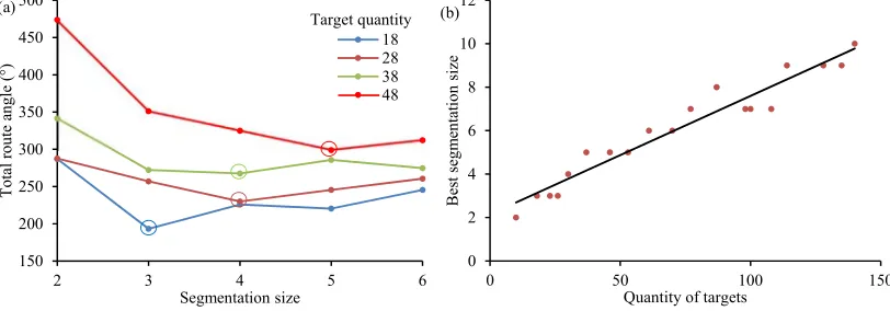
For the “segmentation” algorithm, it can be seen from Fig. 11(a) that the segmentation size (quantity of targets in one block) influenced route length significantly. When target quantities were 18, 28, 38 and 48, the best segmentation size (circled) were 3, 4, 4, and 5, respectively. Therefore, it seems that the best segmentation size did have a relationship with targets quantity.
Fig. 11. Relationships of total route angle, targets quantity and segmentation size: (a) explorative experiment of segmentation size; (b) it is
obvious the best segmentation size increased gradually when target quantity grew.
To identify the exact relationship, numerous simulation experiments were conducted. The results are shown in Fig. 11(b). It indicated that the best segmentation size had a linear relationship with target quantity. The model was fitted as follow:
0.0545 2.1499,R 0.9388
This model could be applied conveniently in applications, which meant that the best segmentation size could be determined quickly when the target quantity is given.
However, the “segmentation” algorithm needed a longer time to compute. Therefore, it was necessary to identify the net time that the “segmentation” algorithm could be reduced by. Assuming the load on the servo was 0.9 Nm, based on the servos’ specification, the speed, and power of servo were 330°/s and 12 W, respectively. Without considering the servo acceleration and deceleration, converting route
y= 19.903x- 95.212 R² = 0.995
y= 13.783x- 17.296 R² = 0.9815
y= 2.5653x+ 141.83 R² = 0.9531
0 500 1000 1500 2000 2500 3000
0 20 40 60 80 100 120 140 160
T otal route angle ( °)
Quantity of targets Random Follow x-axis Segmentation 150 200 250 300 350 400 450 500
2 3 4 5 6
Tot al r oute a ngle (°) Segmentation size 18 28 38 48 Target quantity 0 2 4 6 8 10 12
0 50 100 150
Bes t s egm entat ion siz e
Quantity of targets
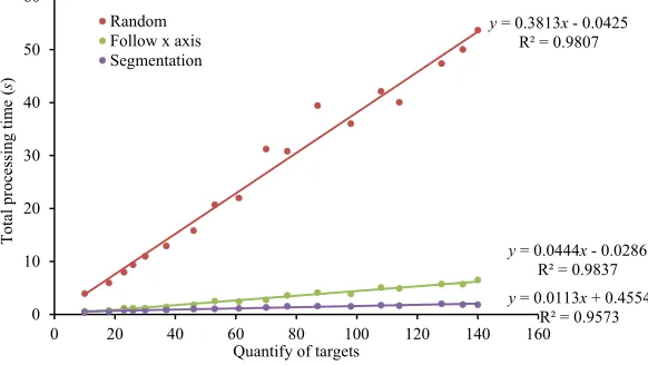
angle into time, based on speed and also including computer computation time, a comparison of total processing time for the three methods is shown in Fig. 12. “Random” needed to calculate 100 different paths, so it had the longest computation time. From the figure, it is clear that the total processing times of “segmentation” and “follow x-axis” were much shorter than “random”. The three methods were linearly modelled and produced high correlation coefficients, although some points of random method had fluctuated. A population of 140 randomly generated weed positions were generated and the three methods were compared, as seen if Fig.12.. The “follow x-axis” reduced time significantly, whereas “segmentation” reduced the time taken even more.
Fig. 12. Comparison of total processing time: all of the methods were linearly modelled. It is clear that the “segmentation” algorithm was the
fastest.
2.2 Control strategy of continuous static weeding
In static weeding, the platform moved to an untreated area and stopped during treatment before moving on to the next untreated area. This method has the advantage of being more accurate as the targets were not moving between machine vision analysis and laser treatment.
Fig. 13 indicates the whole control strategy of continuous static weeding.
After initialisation, the system used image processing to obtain weed centroids. Next, the centroid targets were allocated to each gimbal and sorted by the path planning algorithm. After that the real-world targets of both gimbals were converted into servo angles and sent to the gimbal controller by serial communication and waited for feedback that it had reached the target angles. Once one of the lasers had been pointed on a target and exposure time had been reached, the gimbal controller sent feedback information with this specific gimbal number so that the next target position of this gimbal was released accordingly. This method could enable two gimbals to work in parallel. An image frame was completed when all of the weeds had been treated. After that, a “move” command was sent to the platform controller and waited for feedback that it had reached the destination. The platform controlled itself to move a specific distance (214 mm). The weeding task was executed on the next image area until no weeds were detected. This strategy could control the robot to weed the whole row and stop automatically.
y= 0.3813x- 0.0425 R² = 0.9807
y= 0.0444x- 0.0286 R² = 0.9837 y= 0.0113x+ 0.4554
R² = 0.9573 0
10 20 30 40 50 60
0 20 40 60 80 100 120 140 160
T
otal
proc
essing
tim
e
(
s
)
Quantify of targets Random
Start Initialisation Complete all of the targets ? Image processing Path planning Camera Dual‐manipulator subsystem Weeds detected? Platform control subsystem Stop Enough laser exposure time? Finish moving? Yes No No No Yes Yes Allocating targets to two manipulators according to their coordinates No Ethernet Serial Convert coordinates
into servos’angles
Move platform command Continue for next image frame Serial feedback Serial feedback Serial feedback available ? Feedback from manipulator 1? Release next target of manipulator 1 Release next target of manipulator 2 No Yes Yes No Serial Release the first targets of both manipulators Serial feedback available ? Image data No Yes Yes
Fig. 13. Flowchart of continuous static weeding control strategy.
3. Results[Somethingwrongwiththenumberingsystem]
4.1 Weeding error test
Since it is important to accurately identify the weed target and ensure accurate positioning of the laser, it was necessary to test and evaluate the positional errors. The error analysis was determined by many of factors, such as camera calibration, image processing, platform vibration and installation error, etc. Most importantly, as lasers were directly positioned by the gimbals, their resolution affected the weeding error significantly. In this paper, a simple weeding error experiment was performed as shown in Fig. 14(a). Several papers with some regular green circles, regarded as weeding targets, were placed on the tray. When the robot was weeding along the tray, laser spots on the papers were marked, so the distance between laser spots and circles centres were regarded as weeding errors. As shown in Fig. 14(b), the weeding error had a near normal distribution, so the results seem reliable. The mean of the weeding error was 1.97 mm, with a 0.88 mm standard deviation.
Error (mm)
(a) (b)
C
Fig. 14. Weeding error test and result: (a) weeding error test setup; (b) weeding error distribution
4.2 Weeding efficiency and successful rate
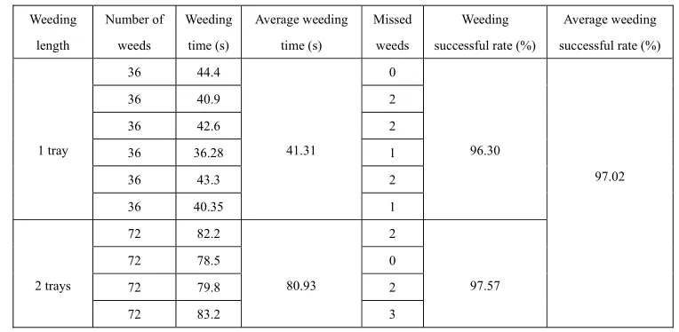
To evaluate the robot performance, a set of weeding experiments were performed. A laser treatment experiment presented by Mathiassen et al. (2006) showed that 90 W, 810 nm laser exposure 640 ms on weeds could control weeds effectively. Therefore, in this paper, the laser was positioned and delayed for a 0.64 s exposure duration. In addition, “eroding and dilating” algorithm was used in this experiment for the segmentation of weeds and crops. As seen in Table 1, the robot was tested on single tray (120 cm length 36 weeds) and double trays (240 cm length 72 weeds), respectively. To ensure high reliability, the weeds were randomly relocated of each test. The results showed that average weeding times for one tray and two trays were 41.31 s and 80.93 s, so the forward weeding speeds were 29 mm/s and 30 mm/s, respectively. The reason of the speed difference was mainly because the platform moved 6 times on one tray while 11 times for two trays. Besides, the robot was demonstrated to have a high average weeding successful rate of 97%.
Table 1
Weeding performance test result.
Weeding length
Number of weeds
Weeding time (s)
Average weeding time (s)
Missed weeds
Weeding successful rate (%)
Average weeding successful rate (%)
1 tray
36 44.4
41.31
0
96.30
97.02
36 40.9 2
36 42.6 2
36 36.28 1
36 43.3 2
36 40.35 1
2 trays
72 82.2
80.93
2
97.57
72 78.5 0
72 79.8 2
72 83.2 3
4. DiscussionsandConclusions
A novel laser weeding prototype robot equipped with a dual-gimbal that can work in parallel was designed and tested. The robot was able to detect weeds in the indoor environments, carry lasers to target at weeds and also control the platform in real-time realising weeding continuously.
be studied further. In terms of time efficiency, all of the colour training, “eroding and dilating” and “shape descriptors” were very fast, with single frame processing times of 0.12 s, 0.0251 s and 0.063 s, respectively, which was meaningful for real-time weeding. Two 2 DOFs gimbals that consisted of four servos and two laser points were developed. They were controlled by a Gimbal controller and could work in parallel. Considering the servo resolution, laser ground resolution (∆x, ∆y) varied from (0.49
mm, 0.49 mm) to (0.54 mm, 0.60 mm).
A new “segmentation” path-planning algorithm for static weeding was proposed and compared. It was demonstrated to be efficient especially when the weed’s quantity was large. The relationships between total shortest route angle and target quantity for “random”, “follow x-axis” and “segmentation” were all fitted by linear models. Based on the models, if there are 40 and 140 targets, compared to “random” and “follow x-axis”, “segmentation” could reduce route angle by approximately 65.1%, 54.2% and 81.4%, 73.8%, respectively. Furthermore, for “segmentation” algorithm, the experiment indicated that the best segmentation size had a linear relationship with target quantity. Therefore, the best segmentation size could be easily and quickly determined based on target quantity. Also, considering computation time, in contrast to “random” and “follow x-axis”, “segmentation” could decrease by 14.3 s and 0.897 s of total processing time with a single gimbal for 40 weeds and 51.3 s and 4.15 s for 140 weeds. Therefore, it was thought that the developed “segmentation” algorithm has the potential to be widely used in fast path-planning for the travelling sales man problem.
Finally, two performance tests were conducted. The weeding error test showed that the mean of the weeding error was 1.97 mm, with a 0.88 mm standard deviation. Another whole process experiment indicated that the weeding speed was 29.66 mm/s for two trays (240 cm length, 72 weeds and 0.64 s laser exposure/weed), with a weeding success rate of 97%.
However, the robot still has some limitations. First, the low-cost platform could not be controlled precisely and did not have a complete navigation system. Secondly, the machine vision subsystem could not distinguish plants if they were touching and also had similar areas at the same time. Finally, static weeding speed was still not potentially as fast as continuous weeding.
Conflictsofinterest
The authors declare that there are no conflicts of interest regarding the publication of this paper.
Acknowledgements
This research was funded by Harper Adams University. The students were supported by China Scholarship Council. We would like to acknowledge technical support from Harper Adams University technicians and research assistants, especially for Mr. Kit Franklin, Mr. Jonathan Gill, and Mr. Michael Warbrick.
References
Ahmad, M T. 2012. Development of an automated mechanical intra-row weeder for vegetable crops. Master Degree Thesis. Ames, Iowa: Iowa State University. DOI:
http://lib.dr.iastate.edu/cgi/viewcontent.cgi?article=3285&context=etd
Akshatha P.S., Vasudha V. and Tanupriya C. 2013. Open Loop Travelling Salesman Problem using Genetic Algorithm. International Journal of Innovative Research in Computer and
Communication Engineering, 1(1), pp.112-116. DOI: https://www.omicsonline.org/scholarly-articles/open-loop-travelling-salesman-problem-usinggenetic-algorithm-42608.html
ISBN 0-691-12993-2. DOI:
http://content.schweitzer-online.de/static/catalog_manager/live/media_files/representation/zd_std_orig__zd_schw_orig/003 /029/406/9780691129938_content_pdf_2.pdf
Bakker, T., Asselt, K., Bontsema, J., Müller, J. and Straten, G., 2010. Systematic design of an autonomous platform for robotic weeding. Journal of Terramechanics, 47(2), pp.63-73. DOI: http://www.sciencedirect.com/science/article/pii/S0022489809000858
Blasco, J., Aleixos, N., Roger, J.M., Rabatel, G. and Molto, E., 2002. AE—Automation and Emerging Technologies: Robotic Weed Control using Machine Vision. Biosystems Engineering, 83(2), pp.149-157. DOI: http://www.sciencedirect.com/science/article/pii/S1537511002901091
Burgos-Artizzu, X. P., Ribeiro, A., Guijarro, M. and Pajares, G. 2011. Real-time image processing for crop/weed discrimination in maize fields. Computers and Electronics in Agriculture, 75(2), pp.337-346. DOI: http://www.sciencedirect.com/science/article/pii/S0168169910002620 Griepentrog, H.W., Noerremark, M. and Soriano, J.F. 2006, September. Close-to-crop thermal weed
control using a CO2 laser. In Proceedings: CIGR World Congress, Agricultural Engineering for a Better World, Bonn, Germany, 3rd–7th September. DOI:
https://www.uni-hohenheim.de/qisserver/rds?state=medialoader&objectid=6993&application=lsf.
Heisel T., Schou J., Christensen S., and Andreasen C., 2001. Cutting weeds with a CO2 laser. Weed Research, 41(1), pp.19–29. DOI:
http://onlinelibrary.wiley.com/doi/10.1046/j.1365-3180.2001.00212.x/full
Iivarinen, J., Peura, M., Särelä, J. and Visa, A., 1997, September. Comparison of Combined Shape Descriptors for Irregular Objects. In Proceedings of the 8th British Machine Vision Conference, pp.430-439.DOI:
https://pdfs.semanticscholar.org/60b9/a74f38f7f1f36e6c4fa3e690b2c1c1c90841.pdf
Marx, C., Barcikowski, S., Hustedt, M., Haferkamp, H. and Rath, T., 2012. Design and application of a weed damage model for laser-based weed control. Biosystems Engineering, 113(2), pp.148-157. DOI: http://www.sciencedirect.com/science/article/pii/S1537511012001195
Mathiassen, S.K., Bak, T., Christensen, S. and Kudsk, P., 2006. The effect of laser treatment as a weed control method. Biosystems Engineering, 95(4), pp.497-505. DOI:
http://www.sciencedirect.com/science/article/pii/S1537511006002984
Midtiby, H.S., Mathiassen, S.K., Andersson, K.J. and Jørgensen, R.N., 2011. Performance evaluation of a crop/weed discriminating microsprayer. Computers and electronics in agriculture, 77(1), pp.35-40. DOI: http://www.sciencedirect.com/science/article/pii/S0168169911000676 Nadimi, E.S., Andersson, K.J., Jørgensen, R.N., Maagaard, J., Mathiassen, S. and Christensen, S.,
2009. Designing, modeling and controlling a novel autonomous laser weeding system. In 7th World Congress on Computers in Agriculture Conference Proceedings, pp.22-24 June 2009, Reno, Nevada. American Society of Agricultural and Biological Engineers. DOI:
https://elibrary.asabe.org/abstract.asp?aid=29077&t=2&redir=&redirType=
O’Dogherty, M.J., Godwin, R.J., Dedousis, A.P., Brighton, J.L. and Tillett, N.D., 2007. A mathematical model of the kinematics of a rotating disc for inter-and intra-row hoeing. Biosystems engineering, 96(2), pp.169-179.
DOI: http://www.sciencedirect.com/science/article/pii/S1537511006003369
DOI: http://www.sciencedirect.com/science/article/pii/S0168169911002341
Slaughter, D.C., Giles, D.K. and Downey, D., 2008. Autonomous robotic weed control systems: A review. Computers and electronics in agriculture, 61(1), pp.63-78.
DOI: http://www.sciencedirect.com/science/article/pii/S0168169907001688
Tillett, N.D., Hague, T., Grundy, A.C. and Dedousis, A.P., 2008. Mechanical within-row weed control for transplanted crops using computer vision. Biosystems Engineering, 99(2), pp.171-178. DOI: http://www.sciencedirect.com/science/article/pii/S1537511007002668
Underwood, J. P., Calleija, M., Taylor, Z., Hung, C., Nieto, J., Fitch, R. and Sukkarieh, S. 2015. Real-time target detection and steerable spray for vegetable crops. Sydney University. DOI:
http://confluence.acfr.usyd.edu.au/download/attachments/14452007/2015-Underwood-ICRAAgWs-Spray.pdf?version=1&modificationDate=1465979705000&api=v2.
Zhang, Z., 2000. A flexible new technique for camera calibration. IEEE Transactions on pattern analysis and machine intelligence, 22(11), pp.1330-1334.