Counting and Exploring Sizes of Markov Equivalence Classes
of Directed Acyclic Graphs
Yangbo He [email protected]
Jinzhu Jia [email protected]
LMAM, School of Mathematical Sciences, LMEQF, and Center for Statistical Science Peking University, Beijing 100871, China
Bin Yu [email protected]
Departments of Statistics and EECS
University of California at Berkeley, Berkeley, CA 94720
Editor:Isabelle Guyon and Alexander Statnikov
Abstract
When learning a directed acyclic graph (DAG) model via observational data, one gener-ally cannot identify the underlying DAG, but can potentigener-ally obtain a Markov equivalence class. The size (the number of DAGs) of a Markov equivalence class is crucial to infer causal effects or to learn the exact causal DAG via further interventions. Given a set of Markov equivalence classes, the distribution of their sizes is a key consideration in devel-oping learning methods. However, counting the size of an equivalence class with many vertices is usually computationally infeasible, and the existing literature reports the size distributions only for equivalence classes with ten or fewer vertices.
In this paper, we develop a method to compute the size of a Markov equivalence class. We first show that there are five types of Markov equivalence classes whose sizes can be formulated as five functions of the number of vertices respectively. Then we introduce a new concept of a rooted sub-class. The graph representations of rooted subclasses of a Markov equivalence class are used to partition this class recursively until the sizes of all rooted sub-classes can be computed via the five functions. The proposed size counting is efficient for Markov equivalence classes of sparse DAGs with hundreds of vertices. Finally, we explore the size and edge distributions of Markov equivalence classes and find experimentally that, in general, (1) most Markov equivalence classes are half completed and their average sizes are small, and (2) the sizes of sparse classes grow approximately exponentially with the numbers of vertices.
Keywords: directed acyclic graphs, Markov equivalence class, size distribution, causality
1. Introduction
equivalent DAGs; however, it is possible to learn the Markov equivalence class that contains these equivalent DAGs (Pearl, 2000; Spirtes et al., 2001). This has led to many works that try to learn a Markov equivalence class or to learn causality based on a given Markov equivalence class from observational or experimental data (Castelo and Perlman, 2004; Chickering, 2002; He and Geng, 2008; Maathuis et al., 2009; Perlman, 2001).
The size of a Markov equivalence class is the number of DAGs in the class. This size has been used in papers to design causal learning approaches or to evaluate the “complex-ity” of a Markov equivalence class in causal learning. For example, He and Geng (2008) proposes several criteria, all of which are defined on the sizes of Markov equivalence classes, to minimize the number of interventions; this minimization makes helpful but expensive interventions more efficient. Based on observational data, Maathuis et al. (2009) introduces a method to estimate the average causal effects of the covariates on the response by consid-ering the DAGs in the equivalence class; the size of the class determines the complexity of the estimation. Chickering (2002) shows that causal structure search in the space of Markov equivalence class models could be substantially more efficient than that in the space of DAG models if most sizes of Markov equivalence classes are large.
The size of a small Markov equivalence class is usually counted via traversal methods that list all DAGs in the Markov equivalence class (Gillispie and Perlman, 2002). However, if the class is large, it may be infeasible to list all DAGs. For example, as we will show later in our experiments, the size of a Markov equivalence class with 50 vertices and 250 edges could be greater than 1024. To our knowledge, there are no efficient methods to compute the size of a large Markov equivalence class; approximate proxies, such as the number of vertices and the number of spanning trees related to the class, have been used instead of the exact size in the literature (Chickering, 2002; He and Geng, 2008; Meganck et al., 2006).
Computing the size of a Markov equivalence class is the focus of this article. We first discuss Markov equivalence classes whose sizes can be calculated just through the numbers of vertices and edges. Five explicit formulas are given to obtain the sizes for five types of Markov equivalence classes respectively. Then, we introduce rooted sub-classes of a Markov equivalence class and discuss the graphical representations of these sub-classes. Finally, for a general Markov equivalence class, we introduce a counting method by recursively partitioning the Markov equivalence class into smaller rooted sub-classes until all rooted sub-classes can be counted with the five explicit formulas.
Next, we also report new results about the size and edge distributions of Markov equiv-alence classes for sparse graphs with hundreds of vertices. By using the proposed size counting method in this paper and an MCMC sampling method recently developed by He et al. (2013a,b), we experimentally explore the size distributions of Markov equivalence classes with large numbers of vertices and different levels of edge sparsity. In the literature, the size distributions are studied in detail just for Markov equivalence classes with up to 10 vertices by traversal methods (Gillispie and Perlman, 2002).
2. Markov Equivalence Class
A graphG consists of a vertex setV and an edge setE. A graph is directed (undirected) if all of its edges are directed (undirected). A sequence of edges that connect distinct vertices inV, say{v1,· · ·, vk}, is called a path fromv1 tovk if eithervi →vi+1 orvi−vi+1 is inE
fori= 1,· · ·, k−1. A path ispartially directed if at least one edge in the path is directed. A path is directed (undirected) if all edges are directed (undirected). Acycleis a path from a vertex to itself.
A directed acyclic graph (DAG) D is a directed graph without any directed cycle. Let
V be the vertex set of D and τ be a subset of V. The induced subgraph Dτ of D overτ, is defined to be the graph whose vertex set is τ and whose edge set contains all of those edges of D with two end points in τ. A v-structure is a three-vertex induced subgraph of
D like v1 → v2 ← v3. A graph is called a chain graph if it contains no partially directed
cycles. The isolated undirected subgraphs of the chain graph after removing all directed edges are the chain components of the chain graph. Achord of a cycle is an edge that joins two nonadjacent vertices in the cycle. An undirected graph is chordal if every cycle with four or more vertices has a chord.
A graphical model is a probabilistic model for which a DAG denotes the conditional independencies between random variables. A Markov equivalence class is a set of DAGs that encode the same set of conditional independencies. Let the skeleton of an arbitrary graphG be the undirected graph with the same vertices and edges as G, regardless of their directions. Verma and Pearl (1990) proves that two DAGs are Markov equivalent if and only if they have the same skeleton and the same v-structures. Moreover, Andersson et al. (1997) shows that a Markov equivalence class can be represented uniquely by anessential graph.
Definition 1 (Essential graph) The essential graph of a DAG D, denoted as C, is a graph that has the same skeleton as D, and an edge is directed inC if and only if it has the same orientation in every equivalent DAG ofD.
It can be seen that the essential graph C of a DAGD has the same skeleton as D and keeps the v-structures of D. Andersson et al. (1997) also introduces some properties of an essential graph.
Lemma 2 (Andersson et al. (1997)) Let C be an essential graph of D. Then C is a chain graph, and each chain component Cτ of C is an undirected and connected chordal graph, where τ is the vertex set of the chain component Cτ.
Let SizeMEC(C) denote the size of the Markov equivalence class represented byC (size ofCfor short). Clearly, SizeMEC(C) = 1 ifCis a DAG; otherwiseCmay contain more than one chain component, denoted byCτ1,· · ·,Cτk. From Lemma 2, each chain component is an undirected and connected chordal graph (UCCG for short); and any UCCG is an essential graph that represents a Markov equivalence class (Andersson et al., 1997). We can calculate the size ofC by counting the DAGs in Markov equivalence classes represented by its chain components using the following equation (Gillispie and Perlman, 2002; He and Geng, 2008):
SizeMEC(C) = k
Y
i=1
To count the size of Markov equivalence class represented by a UCCG, we can generate all equivalent DAGs in the class. However, when the number of vertices in the UCCG is large, the number of DAGs in the corresponding Markov equivalence class may be huge, and the traversal method proves to be infeasible to count the size. This paper tries to solve this counting problem for Markov equivalence classes of DAGs with hundred of vertices.
3. The Size of Markov Equivalence Class
In order to obtain the size of a Markov equivalence class, it is sufficient to compute the size of Markov equivalence classes represented by undirected and connected chordal graph (UCCGs) according to Lemma 2 and Equation (1). In Section 3.1, we discuss Markov equiv-alence classes represented by UCCGs whose sizes are functions of the number of vertices. Then in Section 3.2.1, we provide a method to partition a Markov equivalence class into smaller subclasses. Using these methods, finally in Section 3.2.2, we propose a recursive approach to calculate the size of a general Markov equivalence class.
3.1 Size of Markov Equivalence Class Determined by the Number of Vertices
Let Up,n be an undirected and connected chordal graph (UCCG) with p vertices and n edges. Clearly, the inequalityp−1≤n≤p(p−1)/2 holds for any UCCG Up,n. WhenUp,n is a tree,n=p−1 and when Up,nis a completed graph, n=p(p−1)/2. Given pand n, in some special cases, the size of a UCCG Up,n is completely determined by p. For example, it is well known that a Markov equivalence class represented by a completed UCCG withp
vertices containsp! DAGs. Besides the Markov equivalence classes represented by completed UCCGs, there are five types of UCCGs whose sizes are also functions ofp. We present them as follows.
Theorem 3 Let Up,n be a UCCG with p vertices and n edges. In the following five cases,
the size of the Markov equivalence class represented byUp,n is determined by p.
1. If n=p−1, we have SizeMEC(Up,n) =p.
2. If n=p, we have SizeMEC(Up,n) = 2p.
3. If n=p(p−1)/2−2, we haveSizeMEC(Up,n) = (p2−p−4)(p−3)!.
4. If n=p(p−1)/2−1, we haveSizeMEC(Up,n) = 2(p−1)!−(p−2)!.
5. If n=p(p−1)/2, we have SizeMEC(Up,n) =p!.
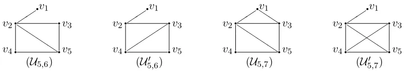
For the UCCGs other than the above five cases, it seems that the sizes of the correspond-ing Markov equivalence classes cannot be completely determined by the numbers of vertices and edges; the sizes of these Markov equivalence classes may depend on the exact essential graphs. Below, we display several classes of this kind forn=p+ 1 or n=p(p−1)/2−3 in Example 1.
Example 1. Figure 1 displays four UCCGs. Both U5,6 and U50,6 have 6 edges, and
both U5,7 and U0
5,7 have 7 edges. We have that SizeMEC(U5,6) = 13, SizeMEC(U50,6) = 12,
SizeMEC(U5,7) = 14 and SizeMEC(U50,7) = 30. Clearly, in these cases, the sizes of Markov
q
q q
q q
v1 v2 v3 v4 v5
Q Q Q Q
(U5,6)
q
q q
q q
v1 v2 v3 v4 v5
(U50,6)
q
q q
q q
v1 v2 v3 v4 v5
Q Q Q Q Q Q
(U5,7)
q
q q
q q
v1 v2 v3 v4 v5
Q Q Q Q
(U50,7) Figure 1: Examples that UCCGs with the same number of edges have different sizes.
3.2 Size of a General Markov Equivalence Class
In this section, we introduce a general method to count the size of a Markov equivalence class. We have shown in Theorem 3 that there are five types of Markov equivalence classes whose sizes can be calculated with five formulas respectively. For one any other Markov equivalence class, we will show in this section that it can be partitioned recursively into smaller subclasses until the sizes of all subclasses can be calculated with the five formulas above. We first introduce the partition method and the graph representation of each sub-class in Section 3.2.1. Then provide a size counting algorithm for one arbitrary Markov equivalence class in Section 3.2.2. The proofs of all results in this section can be found in the Appendix.
3.2.1 Methods to Partition a Markov Equivalence Class
Let U be a UCCG, τ be the vertex set of U and let D be a DAG in the equivalence class represented by U. A vertexv is aroot of Dif all directed edges adjacent to v are out ofv, and Dis v-rooted ifvis a root of D. To count DAGs in the class represented by U, below, we show that all DAGs can be divided into different groups according to the roots of the DAGs and then we calculate the numbers of the DAGs in these groups separately. Each group is called as a rooted sub-class defined as follows.
Definition 4 (a rooted sub-class) Let U be a UCCG over τ and v ∈τ. We define the
v-rooted sub-class of U as the set of all v-rooted DAGs in the Markov equivalence class represented by U.
The following theorem provides a partition of a Markov equivalence class represented by a UCCG and the proof can be found in Appendix.
Theorem 5 (a rooted partition) Let U be a UCCG over τ = {v1,· · ·, vp}. For any
i ∈ {1,· · ·, p}, the vi-rooted sub-class is not empty and this set of p sub-classes forms a
disjoint partition of the set of all DAGs represented by U.
Below we describe an efficient graph representation of v-rooted sub-class. One reason to this graph representation is that for any v ∈ τ, the number of DAGs in the v-rooted sub-class might be extremely huge and it is computationally infeasible to list all v-rooted DAGs in this sub-class. Using all DAGs in whichvis a root, we construct a rooted essential graph in Definition 6.
Definition 6 (rooted essential graph) Let U be a UCCG. Thev-rooted essential graph of U, denoted by U(v), is a graph that has the same skeleton as U, and an edge is directed
From Definition 6, a rooted essential graph has more directed edges than the essential graph U since the root introduces some directed edges. Algorithm 3 in Appendix shows how to generate thev-rooted essential graph of a UCCGU. We display the properties of a rooted essential graph in Theorem 7 and the proof can be found in Appendix.
Theorem 7 Let U be a UCCG and U(v) be a v-rooted essential graph of U defined in
Definition 6. The following three properties hold forU(v):
1. U(v) is a chain graph,
2. every chain component Uτ(v0) of U(v) is chordal, and
3. the configuration v1 →v2−v3 does not occur as an induced subgraph of U(v).
Moreover, there is a one-to-one correspondence between v-rooted sub-classes and v-rooted essential graphs, so U(v) can be used to represent uniquely thev-rooted sub-class ofU.
From Theorem 7, we see that the number of DAGs in a v-rooted essential graph U(v)
can be calculated by Equation (1) which holds for any essential graph. To use Equation (1), we have to generate all chain components of U(v). Below we introduce an algorithm
calledChainCom(U,v) in Algorithm 1 to generate U(v) and all of its chain components. Algorithm 1:ChainCom(U, v)
Input: U, a UCCG; v, a vertex of U.
Output: v−rooted essential graph of U and all of its chain components.
1 Set A={v},B=τ\v,G=U and O=∅ 2 while B is not empty do
3 SetT ={w:w inB and adjacent toA} ;
4 Orient all edges betweenAand T as c→tin G, where c∈A, t∈T;
5 repeat
6 foreach edge y−z in the vertex-induced subgraph GT do
7 if x→y−z in G and x and z are not adjacent in G then
8 Orienty−z toy→z inG
9 until no more undirected edges in the vertex-induced subgraph GT can be
oriented;
10 SetA=T and B =B\T;
11 Append all isolated undirected graphs inGT toO;
12 return G andO
We show that Algorithm 1 can generate rooted essential graph and the chain components of this essential graph correctly in the following theorem.
Theorem 8 Let U be a UCCG and let v be a vertex in U. LetO and G be the outputs of Algorithm 1 givenU and v. Then G is the v-rooted essential graph G=U(v) of U and O is
The following example displays rooted essential graphs of a UCCG and illustrates how to implement Algorithm 1 to construct a rooted essential graph and how to generate all DAGS in the corresponding rooted sub-classes.
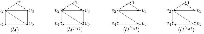
Example 2. Figure 2 displays an undirected chordal graph U and its rooted essential graphs. There are five rooted essential graphs {U(vi)}
i=1,···,5. We need to construct only U(v1),U(v2) and U(v3) sinceU(v4) and U(v5) are symmetrical to U(v1) and U(v3) respectively.
Clearly, they satisfy the conditions shown in Theorem 7. Given U in Figure 2, U(v1) is
constructed according to Algorithm 1 as follows: (1) setT ={v2, v3} in which vertices are
adjacent to v1, orient v1−v2, v1−v3 tov1→v2, v1 →v3 respectively; (2) set T ={v4, v5}
in which vertices are adjacent to {v2, v3}, orient v2−v4, v2−v5, v3−v5 to v2 → v4, v2 → v5, v3 → v5 respectively; (3) orient v5 −v4 to v5 → v4 because v3 → v5 −v4 occurs but v3 and v4 are not adjacent. By orientating the undirected edges of the chain components
of a rooted essential graph with the constraint that no new v-structures and directed cycle occur, we can generate all DAGS in the corresponding sub-class (He and Geng, 2008; Meek, 1995; Verma, 1992). For example, consider U(v1) in Figure 2, we get twov
1-rooted DAGs
by orientingv2−v3 tov2→v3 orv2 ←v3.
q
q q
q q
v1 v2 v3 v4 v5
Q Q Q Q Q Q
(U)
q
q q
q q
v1 v2 v3 v4 v5
+ QQs
? ? Q Q Q Q s
(U(v1))
q
q q
q q
v1 v2 v3 v4 v5
3 Q Q ? Q Q Q Q s
(U(v2))
q
q q
q q
v1 v2 v3 v4 v5
Q Q k ? ? Q Q Q Q
(U(v3))
Figure 2: An undirected chordal graphU and its rooted essential graphs: U(v1),U(v2), and U(v3).
Now we can partition a Markov equivalence class represented by a UCCG into disjoint sub-classes, each of which can be represented by a rooted essential graph. In the next section, we will show how to recursively implement these partitions until the sizes of the subclasses or their essential graphs can be calculated with the five formulas in Theorem 3.
3.2.2 Calculating the Size of a Markov Equivalence Class
Let U be an undirected and connected chordal graph (UCCG) over τ. For any v ∈ τ, SizeMEC(U(v)) denotes the number of DAGs in v-rooted sub-class of U. According to
Theorem 5, the size ofU can be calculated via the following corollary.
Corollary 9 Let U be a UCCG over τ = {vi}i=1,···,p. We have SizeMEC(U(vi)) > 1 for
i= 1,· · ·, pand
SizeMEC(U) = p
X
i=1
SizeMEC(U(vi)). (2)
This corollary shows that the size of Markov equivalence class represented by U can be calculated via the sizes of smaller sub-classes represented by {U(vi)}
Example 3. Consider again the undirected chordal graphU in Figure 2, SizeMEC(U) can be calculated as P5
i=1SizeMEC(U(vi)) according to Corollary 9. The sizes of the five
subclasses represented byU(v1),· · ·,U(v5) are 2,4,3,2,3 respectively. Therefore, we can get
that SizeMEC(U) = 2 + 4 + 3 + 2 + 3 = 14.
According to Theorem 7, for any i ∈ {1,· · ·, p}, the vi-rooted essential graph U(vi)
is a chain graph. If U(vi) is not directed, each of their isolated undirected subgraphs is a
UCCG. Recall that we can calculate the size of a Markov equivalence class through its chain components using Equation (1), similarly, we can calculate the size of vi-rooted sub-class of U with its isolated UCCGs as follows.
Corollary 10 Let U(vi) be a v
i-rooted equivalent sub-class ofU defined in Definition 6 and
{Uτj(vi)}j=1,···,l be the isolated undirected chordal sub-graphs ofU(vi) over the vertex set τj for
j= 1,· · ·, l. We have
SizeMEC(U(vi)) = l
Y
j=1
SizeMEC(Uτj(vi)). (3)
Since {Uτj(vi)}j=1,···,l are UCCGs according to Theorem 7, SizeMEC(Uτj(vi)) can be calcu-lated again via Equation (2) in Corollary 9 recursively. In this iterative approach, Equation (2) and Equation (3) are used alternately to calculate the sizes of equivalence classes rep-resented by an undirected essential graph and a rooted essential graph.
Now in Algorithm 2 we present an enumeration to give SizeMEC(U). Corollary 11 shows that the enumeration returns the size correctly. For any essential graph C, we can calculate the size of Markov equivalence class represented by C according to Equation (1) and Algorithm 2.
Algorithm 2:SizeMEC(U)
Input: U: a UCCG.
Output: the size of Markov equivalence classes represented byU
1 Let pand n be the numbers of vertices and edges inU; 2 switch ndo
3 casep−1return p; 4 casepreturn 2p;
5 casep(p−1)/2−2 return (p2−p−4)(p−3)!; 6 casep(p−1)/2−1 return 2(p−1)!−(p−2)!; 7 casep(p−1)/2 return p!;
8 for j←1 to pdo
9 {U1,· · ·,Ulj} ← ChainCom(U, vj);
10 sj ←Q
lj
i=1 SizeMEC(Ui)
11 return Ppi=1si
The complexity of calculating SizeMEC(U) via Algorithm 2 depends on the number of times this recursive function is called. Our experiments in the next section show that when the number of vertices in U is small, or when the number is large but U is sparse, our proposed approach is efficient. However, whenU is large and dense, the proposed approach may be computational infeasible since calculating SizeMEC(U) via Algorithm 2 may require a very deep recursion. In the worst case, the time complexity of Algorithm 2 might beO(p!). For example, it might be extremely time-consuming to count SizeMEC(U) via Algorithm 2 when U is a UCCG with large p vertices andp(p−1)/2−3 edges. Fortunately, according to the experimental results in He et al. (2013a), the undirected and connected chordal sub-graphs in sparse essential sub-graphs with hundreds of vertices are mostly small. This implies that our approach may be valuable for size counting in most situations of causal learning based on sparse graphical models.
In the next section, we demonstrate our approach experimentally and explore the size and edge distributions of Markov equivalence classes in sparse graphical models.
4. Experimental Results
We conduct experiments to evaluate the proposed size counting algorithms in Section 4.1, and then to study sizes of Markov equivalence classes in Section 4.2. The main contributions of these experiments are as follows.
1. Our proposed approach can calculate the size of classes represented by a UCCG with a few vertices (p < 15) in seconds on a laptop of 2.7GHz and 8G RAM. When the number of vertices is large, our approach is also efficient for the graphs with a sparsity constraint.
2. For the essential graphs with a sparsity constraint, the sizes of the corresponding Markov equivalence classes are nearly exponential in p. This explains the result in Chickering (2002) that causal structure search in the space of Markov equivalence class models could be substantially more efficient than the search in the space of DAG models for learning sparse graphical models.
3. In the set of all Markov equivalence classes of DAGs with p vertices, most graphs are half-completed (nearlyp2/4 edges exist) and the Markov equivalent classes repre-sented by these graphs have small average sizes. This is the reason why all Markov equivalence classes have small average sizes (approximately 3.7 reported by Gillispie and Perlman (2002)) even though sparse Markov equivalence classes are huge.
4.1 Calculating the Size of Classes Represented by UCCGs
Let Unp∗ be the set of Markov equivalence classes with p vertices and n edges. The graphs in Unp∗ are sparse ifn is a small multiple of p. We generate random choral graphs in Unp∗ as follows. First, we construct a tree by connecting two vertices (one is sampled from the connected vertices and the other from the isolated vertices) sequentially until all
pvertices are connected. Then we randomly insert an edge such that the resulting graph is chordal, repeatedly until the number of edges reachesn. Repeating this procedureN times, we obtainN samples from Uip∗ for each i∈[p−1, n].
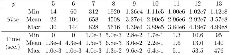
We first consider the undirected chordal graphs with 5 to 13 vertices. Our experiments onUnp∗for anyn < p(p−1)/2−3 show that it is most time-consuming to calculate the size of UCCGs whenn=p(p−1)/2−3. Based on the samples fromUpn∗ wheren=p(p−1)/2−3, we report in Table 1 the the maximum, the minimum and the average of the sizes of Markov equivalence classes and the time to count them. We see that the size is increasing exponentially inpand the proposed size-counting algorithm is computationally efficient for undirected chordal graphs with a few vertices.
p 5 6 7 8 9 10 11 12 13
Size
Min 14 60 312 1920 1.36e4 1.11e5 1.00e6 1.02e7 1.12e8
Mean 22 104 658 4508 3.27e4 2.90e5 2.96e6 2.92e7 3.57e8
Max 30 144 828 5616 4.39e4 3.89e5 3.84e6 4.19e7 4.99e8
Time (sec.)
Min 0 0 1.0e-3 5.0e-3 2.8e-2 1.7e-1 1.3 10.6 95
Mean 1.3e-4 4.3e-4 1.5e-3 6.8e-3 3.6e-2 2.2e-1 1.6 13.6 140
Max 1.0e-3 1.0e-3 4.0e-3 1.3e-2 9.6e-2 6.4e-1 5.1 53.5 476
Table 1: The size of Markov equivalence class and the time to calculate it via Algorithm 2 based on 105 samples fromUnp∗, wherepranges from 5 to 13 andn=p(p−1)/2−3 (the worst case for classes with pvertices).
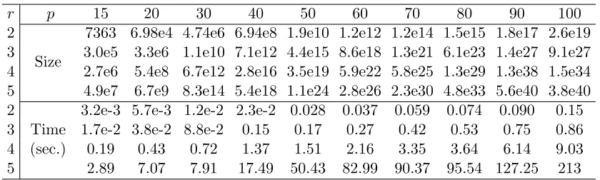
We also study the sets Unp∗ that contain UCCGs with tens of vertices. The number of verticespis set to 15,20,· · ·,100 and the edge constraintm is set torpwherer is the ratio ofmtop. For eachp, we consider four ratios: 2, 3, 4 and 5. The undirected chordal graphs inUrpp ∗are sparse sincer ≤5. Based on 105 samples, we report the average size and time in Table 2. We can see that whenr≤4, the algorithm just takes a few seconds even when the sizes are very huge; when the chordal graphs become denser (r > 4), the algorithm takes more time.
Here we have to point out that the choral graphs generated in this experiment might not be uniformly distributed in the space of chordal graphs and that the averages in Table 1 and Table 2 are not accurate estimations of expectations of sizes and time.
4.2 Size and Edge Distributions of Markov Equivalence Classes
r p 15 20 30 40 50 60 70 80 90 100 2
Size
7363 6.98e4 4.74e6 6.94e8 1.9e10 1.2e12 1.2e14 1.5e15 1.8e17 2.6e19
3 3.0e5 3.3e6 1.1e10 7.1e12 4.4e15 8.6e18 1.3e21 6.1e23 1.4e27 9.1e27
4 2.7e6 5.4e8 6.7e12 2.8e16 3.5e19 5.9e22 5.8e25 1.3e29 1.3e38 1.5e34
5 4.9e7 6.7e9 8.3e14 5.4e18 1.1e24 2.8e26 2.3e30 4.8e33 5.6e40 3.8e40
2
Time (sec.)
3.2e-3 5.7e-3 1.2e-2 2.3e-2 0.028 0.037 0.059 0.074 0.090 0.15
3 1.7e-2 3.8e-2 8.8e-2 0.15 0.17 0.27 0.42 0.53 0.75 0.86
4 0.19 0.43 0.72 1.37 1.51 2.16 3.35 3.64 6.14 9.03
5 2.89 7.07 7.91 17.49 50.43 82.99 90.37 95.54 127.25 213
Table 2: The average size of Markov equivalence classes and average counting time via Algorithm 2 are reported based on 105 samples from Uprp ∗, where p ranges from 15 to 100.
of Markov equivalence classes of interest. In Section 4.2.1, we study the size and edge distributions of Markov equivalence classes with tens of vertices, and in Section 4.2.2, we provide the size distributions of Markov equivalence classes with hundred of vertices under sparsity constraints.
4.2.1 Size and Edge Distribution of Markov Equivalence Classes
In this section, we discuss the distributions of Markov equivalence classes on their sizes and number of edges. We use “size distribution” for the distribution on sizes of Markov equivalence classes, and “edge distribution” for the distribution on the number of edges. First, we consider the number of edges of Markov equivalence classes with p vertices for 10 ≤ p < 20. Then, we focus on the size and edge distribution of Markov equivalence classes with 20 vertices. Finally, we explore the size distributions of Markov equivalence classes with different numbers of edges to show how size distributions change with increasing numbers of edges.
The numbers of edges in the Markov equivalence classes with pvertices range from 0 to
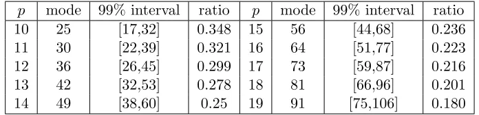
p(p−1)/2. Based on a Markov chain with length of 106 for eachp, we display in Table 3 the modes and 99% intervals of edge distributions of Markov equivalence classes withpvertices for 10 ≤ p < 20. The mode is the number that appears with the maximum probability, 99% interval is the shortest interval that covers more than 99% of Markov equivalence classes. The ratios that measure the fraction of 99% interval to p(p−1)/2 + 1 are also given. For example, consider the edge distribution of Markov equivalence classes with 10 vertices; we see that 99% of Markov equivalence classes have between 17 and 32 edges. The ratio is 16/46 ≈0.348, where the number 16 is the length of the 99% interval [17,32] and 46 is the length of the edge distribution’s support [0,45]. From the 99% intervals and the corresponding ratios, we see that the numbers of edges of Markov equivalence classes are sharply distributed aroundp2/4, and these distributions become sharper with increasing of p. This result is reasonable since the number of skeletons of essential graphs with k edges is p(p−k1)/2
, and thek-combination reaches maximum around k=p2/4.
p mode 99% interval ratio p mode 99% interval ratio
10 25 [17,32] 0.348 15 56 [44,68] 0.236
11 30 [22,39] 0.321 16 64 [51,77] 0.223
12 36 [26,45] 0.299 17 73 [59,87] 0.216
13 42 [32,53] 0.278 18 81 [66,96] 0.201
14 49 [38,60] 0.25 19 91 [75,106] 0.180
Table 3: The edge distributions of Markov equivalence classes withp vertices for 10≤p <
20. The mode is the number that appears with the maximum probability, the 99% interval covers more than 99% of Markov equivalence classes, ratio is the fraction of the length of the 99% interval to the length of the support of edge distribution.
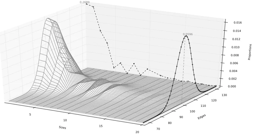
planes are also shown. The black dashed line is the size distribution and the black solid line is the edge distribution of Markov equivalence classes. According to the marginal size distribution, we see that most of the Markov equivalence classes with 20 vertices have small sizes. For example, 26.89% of Markov equivalence classes are of size one; the proportion of Markov equivalence classes with size ≤ 10 is greater than 95%. We also see that the marginal edge distribution of Markov equivalences is concentrated around 100(= 202/4). The proportion of Markov equivalence classes with 20 vertices and 100 edges is nearly 6%. To study how the size distribution changes with the number of edges, we consider Markov equivalence classes with 100 vertices and nedges for differentn.
Figure 4 displays the size distribution of Markov equivalence classes with 100 vertices and n edges for n = 10,50,100,200,400,600,1000,1500,2000 and 2500, respectively. We see that the sizes of Markov equivalence classes are very small when the number of edges is close top2/4 = 2500. For example, whenn∈(1000,2500), the median of the sizes is no more than 4. These results shed light on why the Markov equivalence classes have a small average size (approximately 3.7 reported by Gillispie and Perlman (2002)).
4.2.2 Size Distributions of Markov Equivalence Classes with Sparsity Constraints
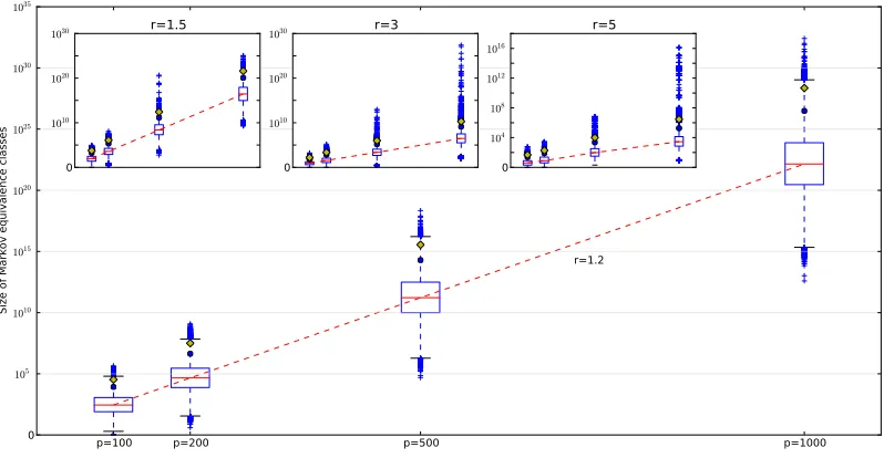
We study Markov equivalence classes withpvertices andnvertices. The number of vertices
p is set to 100,200,500 or 1000 and the maximum number of edgesn is set to rp where r
is the ratio of n top. For each p, we consider four ratios: 1.2, 1.5, 3 and 5. The essential graphs with pvertices and rpedges are sparse since r≤5. In each simulation, givenp and
r, a Markov chain with length of 106 Markov equivalence classes is generated.
There are sixteen distributions, each of which is calculated with 106essential graphs. We plot the four distributions forr= 1.2 in the main window, and the other 12 distributions for
Sizes 5
10
15
20
Edges
70 80
90 100
110 120 130
Proportions
0.000 0.002 0.004 0.006 0.008 0.010 0.012 0.014 0.016 0.2689
0.0596
Figure 3: The surface displays the distribution of the Markov equivalence classes with 20 vertices. Two rescaled marginal distributions are shown in the planes. The black dashed line is the size distribution and the black solid line is the edge distribution of Markov equivalence classes.
These results suggest that, to learn directed graphical models, a searching among Markov equivalence classes might be more efficient than that among DAGs since the number of Markov equivalence classes is much less than the number of DAGs when the graphs of interest are sparse.
5. Conclusions and Discussions
n=10 n=50 n=100 n=200 n=400 0
10 102 103 104 105 106
107 Size of MECs with 100 vertices
n=600 n=1000 n=1500 n=2000 n=2500
0 2 4 6 8 10 12
14 Size of MECs with 100 vertices
Figure 4: The size distributions of Markov equivalence classes with pvertices and nedges, wheren= 10,50,100, 200,400, 600, 1000, 1500, 2000 and 2500, respectively.
p=100 p=200 p=500 p=1000
0
105 1010 1015 1020 1025 1030 1035
Size of Markov equivalence classes
r=1.2 0
1010 1020
1030 r=1.5
0
1010 1020
1030 r=3
0
104 108 1012 1016
r=5
Figure 5: Size distributions of Markov equivalence classes with p vertices and at most rp
edges. The lines in the boxes and the two circles above the boxes indicate the medians, the 95th, and the 99th percentiles respectively.
size of a Markov equivalence class is no longer determined by the number of vertices p; it depends on the structure of the corresponding UCCG and our proposed method might be inefficient when p is large. For these cases, it is of interest to develop more efficient algorithm, or formulas, to calculate the size of a general Markov equivalence class in the future work.
Moreover, we use python to implement algorithms and experiments in this paper and the python package can be found at pypi.python.org/pypi/MarkovEquClasses.
Acknowledgments
We are very grateful to Adam Bloniarz for his comments that significantly improved the presentation of our manuscript. We also thank the editors and the reviewers for their helpful comments and suggestions. This work was supported partially by NSFC (11101008, 11101005, 71271211), DPHEC-20110001120113, US NSF grants DMS-1107000, CDS&E-MSS 1228246, ARO grant W911NF-11-1-0114, AFOSR Grant FA 9550-14-0016, and the Center for Science of Information (CSoI, a US NSF Science and Technology Center) under grant agreement CCF-0939370.
Appendix A. Proofs of Results
In this section, we provide the proofs of the main results of our paper. We place the proof of Theorem 3 in the end of Appendix because this proof will use the results in Algorithm 1 and Corollary 9.
Proof of Theorem 5:
We first show that τi-rooted sub-class is not empty. For any vertex τi ∈ τ, we just need to construct a DAG D in which no v-structures occurs and all edges adjacent to v
are oriented out of v. The maximum cardinality search algorithm introduced by Tarjan and Yannakakis (1984) can be used to construct D. Let p be the number of vertices in U, the algorithm labels the vertices from p to 1 in decreasing order. We first label τi with
p. As the next vertex to label, select an unlabeled vertex adjacent to the largest number of previously labeled vertices. We can obtain a directed acyclic graph D by orienting the undirected edges ofU from higher number to lower number. Tarjan and Yannakakis (1984) show that no v-structures occur in D if U is chordal. Hence in D, there is no v-structure and all edges adjacent to v are oriented out ofv. We have thatDis a τi-rooted equivalent DAG of U, thusτi-rooted sub-class is not empty.
To prove that the p sub-classes, τi-rooted sub-classes for i = 1,· · ·, p, form a disjoint partition of Markov equivalence class represented by U, we just need to show that every equivalent DAG of U is in only one ofp sub-classes.
Below, we show that D is not in any other rooted sub-class. Suppose that D is also in another τj-rooted sub-class (i 6= j). Clearly, τi and τj are not adjacent. Since U is connected, we can find a shortest path L = {τi −τk− · · · −τl−τj} from τi to τj with more than one edge. The DAGDis in bothτi-rooted andτj-rooted sub-classes, so we have that vi → vk and vj → vl are in D. Considering all vertices in L, there must be a head to head like · → · ← · in D, and the two heads are not adjacent in D since L is shortest path. Consequently, a v-structure appears in D. This is a contradiction because U is an
undirected chordal graph andDmust be a DAG without v-structures.
Proof of Theorem 7:
Consider the proof of Theorem 6 in He and Geng (2008), we set the intervention variable to be v. If v is a root, Theorem 7 becomes a special case of Theorem 6 in He and Geng
(2008).
Proof of Corollary 9:
Theorem 5 shows that for anyi∈ {1,2,· · ·, p}, theτi-rooted sub-class ofU is not empty and thesepsub-classes form a disjoint partition of Markov equivalence class represented by
U. This implies Corollary 9 directly.
Proof of Corollary 10:
Since{Uτj(vi)}j=1,···,larelisolated undirected chordal sub-graphs ofU(vi), the orientations of the undirected edges in a component is irrelevant to the other undirected components.
This results in Equation (3) follow directly.
Proof of Theorem 8:
We first introduce the following Algorithm 3 that can construct a rooted essential graph.
Algorithm 3: Find the v-rooted essential graph of U
Input: U: an undirected and connected chordal graph; v: a vertex of U.
Output: the v-rooted essential graph ofU
1 Set H=U;
2 for each edge · −v in U do 3 Orient· −vto· ←v in H.
4 repeat
5 foreach edge y−z in H do
Rule 1: if there exists · →y−z in H, and· and z are not adjacent then
Orienty−z toy→zin H
Rule 2: if there exists y→ · →z in H then
Orienty−z toy→zin H
6 until no more undirected edges in H can be oriented; 7 return H
A similar version of Algorithm 3 is used in He and Geng (2008) to construct an essential graph given some directed edges. From the proof of Theorem 6 in He and Geng (2008), we have that the output of Algorithm 3, H, is the v-rooted essential graph of U, that is,
chain graph and its isolated undirected subgraphs are chain components. From Algorithm 1, we know thatO contains all isolated undirected subgraphs ofG.
To prove that the outputG of Algorithm 1 is thev-rooted essential graphU(v) ofU and O is the set of all chain components of U(v), we just need to show that G = H given the
sameU and v.
By comparing Algorithm 1 to Algorithm 3, we find that in Algorithm 1, Rule 1 that is shown in Algorithm 3 is used repeatedly, and in the output G of Algorithm 1, undirected edges can no longer be oriented by the Rule 1. If we further apply Rule 2 in Algorithm 3 to orient undirected edges in G until no undirected edges satisfy the condition in Rule 2. Denote the output asG0. Clearly, the outputG0 is the same asH obtained from Algorithm 3, that is, G0 =H. Therefore, to show G =H, we just need to show G = H0, that is, the condition in Rule 2 does not hold for any undirected edge in G.
In Algorithm 1, we generate a setT in each loop of ”while” and the sequence is denoted by {T1,· · ·, Tn}. SettingT0 ={v}, we have five facts as following
Fact 1 All undirected edges in G occur in the subgraphs over Ti fori= 1,· · ·, n.
Fact 2 All edges inG betweenTi andTi+1 are oriented fromTi toTi+1 fori= 0,· · ·, n−1. Fact 3 There is no edge betweenTi and Tj if|i−j|>1.
Fact 4 There are no v-structures inG.
Fact 5 there is no directed cycle (all edges are directed) in G.
Suppose there exist three vertices x, yandz such that bothy→x→zand y−zoccur inG. Then a contradiction is implied.
Since y−z occurs in G, fromFact 1, there exists a set, denoted as Ti containing both
y and z. Moreover,y→x→z occurs inG, from Fact 2and Fact 3, we have thatx∈Ti. Next we show that x, y and z have the same parents in Ti−1. First, y and z have the
same parents in Ti−1; otherwise y−z will be oriented to a directed edge. Denote by P1
the same parents of y and z in Ti−1 and by P2 the parents of x in Ti−1. Second, for any u∈P1, ifuis not a parent ofx, then z−xinU will be oriented toz→xinGaccording to
Algorithm 1. We have that u is also a parent of x and consequently, P1 ⊆P2. Third, For
any u∈P2,u must be a parent ofy according to Fact 4.
We have that P2 ⊆P1, and finally P2 =P1. We get that neither y → x norx → z is
oriented by any directed edge u→y oru→xwith u∈Ti−1 since P2 =P1.
Let u1 ∈ Ti and u1 → y be the directed edge that orients y−x in U to y → x in G.
Clearly,u1 →y occurs in G, and u1 and x are not adjacent. Sincey−z is not directed in G, u1−z must occur inU. Moreover, x → z occurs in G and u1 and x are not adjacent,
we have that u1−z will be oriented to u1 ←z in G. Clearly, there occurs a directed cycle u1 →y→x→z→u1 inG. This is a contradiction according toFact 5. We have that the
condition of Rule 2 does not hold for any undirected edge in G, and consequently, G =H
holds.
Proof of Corollary 11:
According to Corollary 9, Corollary 10, and Theorem 8, the output is the size of Markov
Proof of Theorem 3:
Proof of (1):
For a UCCG Up,n, if n= p−1, then the graph Up,n is a tree. For any vertex in Up,n, we have that Up,n(v) is a DAG according to Algorithm 1. Thus SizeMEC(Up,n) = 1. Then,(v) according to Corollary 9, SizeMEC(Up,n) =p.
Proof of (2):
For a UCCG Up,n, if n = p, then the graph Up,n has one more edge than tree. Be-cause Up,n is chordal, a triangle occurs in Up,n. For any vertex v in Up,n, we have that SizeMEC(Up,n) = 2. Consequently, we have that SizeMEC((v) U) = 2p according to Corollary 9.
Proof of (3):
Let v1,· · ·, vp be the p vertices of Up,n. There are only two pairs of vertices that are nonadjacent sincep(p−1)/2−2 edges appear inUp,n. We first prove that these two pairs have a common vertex. Supposevi−vj and vk−vldo not occur inUp,nand vi, vj, vk, vlare distinct vertices. Consider the subgraph induced by vi, vj, vk, vl of Up,n. Clearly, the cycle
vi−vk−vj−vl−vi occurs in the induced graph andUp,nis not a chordal graph. We have that the missing two edges in Up,n are likev1−v2−v3.
According to Corollary 9, we have that
SizeMEC(Up,n) = p
X
i=1
SizeMEC(Up,n(vi)).
We first consider U(v1)
p,n . All edges adjacent to v2 inUp,n(v1) are oriented to directed edges whose arrow isv2according to Algorithm 1 sincev2 is a neighbor of all neighbors ofv1, and v1, v2 are not adjacent in Up,n(v1). Removing v2 from Up,n(v1), we have that the induced graph overv1, v3,· · ·, vp is a completed graph. This implies that the induced graph overv3,· · ·, vp is an undirected completed graph withp−2 vertices. Therefore, we haveSizeMEC(U(v1)
p,n ) = (p−2)!.
Similarly, we can get that SizeMEC(U(v3)
p,n ) = (p−2)! since v1 and v3 are symmetric in Up,n.
Consider U(v2)
p,n , according to Algorithm 1, for any vertex vj other than v1 and v3, we
have that v2 → vj, vj → v1 and vj → v3 occur in Up,n(v2), and all other edges in Up,n(v2) are undirected. Therefore, there are two isolated chain components inU(v2)
p,n , one contains the edgex1−x3 and the other is the subgraph induced byv4,· · ·, vp. We have the size of first chain component is 2 and the second is (p−3)! since it is a completed graph with p−3 vertices. According to Corollary 10,SizeMEC(U(v2)
p,n ) = 2(p−3)!. We now consider U(v4)
p,n . According to Algorithm 1, to construct Up,n(v4), we first orient the undirected edges adjacent tov4 inUp,n to directed edges out ofv4. Since v4 is adjacent
to all other vertices in Up,n, there are no subgraphs like v4 → vi −vj with v4 and vj nonadjacent. This results in the chain component ofU(v4)
p,n being a graph withp−1 vertices and (p−1)(p−2)/2−2 edges (onlyv1−v2−v3 missing). We have thatSizeMEC(Up,n(v4)) =
Similarly, we can get thatSizeMEC(U(vi)) =SizeMEC(U
p−1,(p−1)(p−2)/2−2) for anyi≥4
since exchanging the labels of these vertices will not change U. Therefore, we have proved the following formula
SizeMEC(Up,n) = (p−3)SizeMEC(Up−1,(p−1)(p−2)/2−2) + 2(p−2)! + 2(p−3)!,
Finally, we show that
SizeMEC(Up,n) = (p2−p−4)(p−3)!
satisfies the formula and initial condition. First, we haveSizeMEC(U4,4) = (16−8)∗1 = 8.
SupposeSizeMEC(Up,n) = (p2−p−4)(p−3)! holds forp=j−1,
SizeMEC(Uj,j(j−1)/2−2)
= (j−3)SizeMEC(Uj−1,(j−1)(j−2)/2−2) + 2(j−2)! + 2(j−3)!
= (j−3){[(j−1)2−(j−1)−4][(j−1)−3]!}+ 2(j−2)! + 2(j−3)! = [(j−1)2−(j−1)−4 + 2(j−2) + 2](j−3)!
= (j2−j−4)!(j−3)!
As a result,SizeMEC(Up,p(p−1)/2−2) = (p2−p−4)(p−3)! holds forp=j. Proof of (4):
From the condition, only one pair of vertices, denoted byvandu, is not adjacent inUp,n. Consider a v-rooted equivalence sub-class, all undirected edges adjacent to u are oriented to directed edges with arrows pointing to u, and all other edges can be orientated as a completed undirected graph. We have that SizeMEC(Up,n) = ((v) p−2)!. Similarly, we have that SizeMEC(Up,n(u)) = (p−2)!. For any vertex w other than v and u, consider any DAG in thew-rooted equivalent sub-class, all edges adjacent to ware oriented away fromw, and all other edges form a new chain component with p−1 vertices and (p−1)(p−2)/2−1 edges. Consider SizeMEC(Up,p(p−1)/2−1) as a function ofp, denoted byf(p). Whenp = 3, we have f(3) = 3. Hence we have following formula:
f(p) = (p−2)f(p−1) + 2((p−2)!).
Now, we show that
f(p) = 2(p−1)!−(p−2)!
satisfies the formula and initial condition. First, we have f(3) = 2∗2−1 = 3. Suppose
f(p) = 2(p−1)!−(p−2)! holds forp=j−1,
f(j) = (j−2)f(j−1) + 2(j−2)!
= (j−2)(2(j−2)!−(j−3)!) + 2(j−2)! = 2(j−2)(j−2)!−(j−2)! + 2(j−2)! = (j−2)!(2j−3)
= 2(j−1)!−(j−2)!
As a result,f(p) = 2(p−1)!−(p−2)! holds forp=j. Proof of (5):
References
S. A. Andersson, D. Madigan, and M. D. Perlman. A characterization of Markov equivalence classes for acyclic digraphs. The Annals of Statistics, 25(2):505–541, 1997.
R. Castelo and M. D. Perlman. Learning essential graph Markov models from data. Studies in Fuzziness and Soft Computing, 146:255–270, 2004.
D. M. Chickering. Learning equivalence classes of Bayesian-network structures.The Journal of Machine Learning Research, 2:445–498, 2002.
M. Finegold and M. Drton. Robust graphical modeling of gene networks using classical and alternative t-distributions. The Annals of Applied Statistics, 5(2A):1057–1080, 2011.
N. Friedman. Inferring cellular networks using probabilistic graphical models. Science Signaling, 303(5659):799, 2004.
S.B. Gillispie and M.D. Perlman. The size distribution for Markov equivalence classes of acyclic digraph models. Artificial Intelligence, 141(1-2):137–155, 2002.
Yangbo He and Zhi Geng. Active learning of causal networks with intervention experiments and optimal designs. Journal of Machine Learning Research, 9:2523–2547, 2008.
Yangbo He, Jinzhu Jia, and Bin Yu. Reversible mcmc on markov equivalence classes of sparse directed acyclic graphs. The Annals of Statistics, 41(4):1742–1779, 2013a.
Yangbo He, Jinzhu Jia, and Bin Yu. Supplement to “reversible mcmc on markov equivalence classes of sparse directed acyclic graphs”. arXiv preprint arXiv:1303.0632, 2013b.
D. Heckerman, C. Meek, and G. Cooper. A Bayesian approach to causal discovery. Com-putation, Causation, and Discovery, pages 143–67, 1999.
R. Jansen, H. Yu, D. Greenbaum, Y. Kluger, N.J. Krogan, S. Chung, A. Emili, M. Snyder, J.F. Greenblatt, and M. Gerstein. A Bayesian networks approach for predicting protein-protein interactions from genomic data. Science, 302(5644):449, 2003.
M. H. Maathuis, M. Kalisch, and P. B¨uhlmann. Estimating high-dimensional intervention effects from observational data. The Annals of Statistics, 37(6A):3133–3164, 2009. ISSN 0090-5364.
C. Meek. Causal inference and causal explanation with background knowledge. In Proceed-ings of the Eleventh Conference on Uncertainty in Artificial Intelligence, pages 403–410, 1995.
S. Meganck, P. Leray, and B. Manderick. Learning causal bayesian networks from observa-tions and experiments: A decision theoretic approach. InModeling Decisions for Artificial Intelligence, pages 58–69. Springer, 2006.
M.D. Perlman. Graphical model search via essential graphs. Contemporary Mathematics, 287:255–266, 2001.
P. Spirtes, C.N. Glymour, and R. Scheines. Causation, Prediction, and Search. The MIT Press, 2001.
R. E. Tarjan and M. Yannakakis. Simple linear-time algorithms to test chordality of graphs, test acyclicity of hypergraphs, and selectively reduce acyclic hypergraphs. SIAM Journal on Computing, 13:566, 1984.
T. Verma. A linear-time algorithm for finding a consistent expansion of a partially oriented graph,”. Technical report, Technical Report R-180, UCLA Cognitive Systems Laboratory, 1992.