Domain Decomposition Approach for Fast Gaussian Process Regression of Large Spatial Data Sets

Domain Decomposition Approach for Fast Gaussian Process

Regression of Large Spatial Data Sets

Chiwoo Park [email protected]

Department of Industrial and Systems Engineering Texas A&M University

3131 TAMU, College Station, TX 77843-3131, USA

Jianhua Z. Huang [email protected]

Department of Statistics Texas A&M University

3143 TAMU, College Station, TX 77843-3143, USA

Yu Ding [email protected]

Department of Industrial and Systems Engineering Texas A&M University

3131 TAMU, College Station, TX 77843-3131, USA

Editor: Neil Lawrence

Abstract

Gaussian process regression is a flexible and powerful tool for machine learning, but the high computational complexity hinders its broader applications. In this paper, we propose a new ap-proach for fast computation of Gaussian process regression with a focus on large spatial data sets. The approach decomposes the domain of a regression function into small subdomains and infers a local piece of the regression function for each subdomain. We explicitly address the mismatch problem of the local pieces on the boundaries of neighboring subdomains by imposing continuity constraints. The new approach has comparable or better computation complexity as other compet-ing methods, but it is easier to be parallelized for faster computation. Moreover, the method can be adaptive to non-stationary features because of its local nature and, in particular, its use of different hyperparameters of the covariance function for different local regions. We illustrate application of the method and demonstrate its advantages over existing methods using two synthetic data sets and two real spatial data sets.

Keywords: domain decomposition, boundary value problem, Gaussian process regression,

paral-lel computation, spatial prediction

1. Introduction

burden. A new computation scheme is developed in this paper with a focus on large spatial data sets.

Existing approximation methods may be categorized into three schools: matrix approximation, likelihood approximation and localized regression. The first school is motivated by the observation that the inversion of a big covariance matrix is the major part of the expensive computation, and thus, approximating the matrix by a lower rank version will help reduce the computational demand. Williams and Seeger (2000) approximated the covariance matrix by the Nystr¨om extension of a smaller covariance matrix evaluated on M training observations (M≪N). This helps reduce the

computation cost from O(N3)to O(NM2), but this method does not guarantee the positivity of the prediction variance (Qui˜nonero-Candela and Rasmussen, 2005, page 1954).

The second school approximates the likelihood of training and testing points by assuming condi-tional independence of training and testing points, given M artificial points, known as “inducing

in-puts.” Under this assumption, one only needs to invert matrices of rank M for GP predictions rather

than the original big matrix of rank N. Depending on the specific independence assumed, there are a number of variants to the approach: deterministic training conditional (DTC, Seeger et al., 2003), full independent conditional (FIC, Snelson and Ghahramani, 2006), partial independent conditional (PIC, Snelson and Ghahramani, 2007). DTC assumes a deterministic relation between the inducing inputs and the regression function values at training sample locations. An issue in DTC is how to choose the inducing inputs; a greedy strategy has been used to choose the inducing inputs among the training data. FIC assumes that each individual training or test point is conditionally independent of one another once given all the inducing inputs. Under this assumption, FIC enjoys a reduced computation cost of O(NM2)for training and O(M2)for testing. However, FIC will have difficulty in fitting data having abrupt local changes or non-stationary features; see Snelson and Ghahramani (2007). PIC makes a relaxed conditional independence assumption in order to better reflect local-ized features. PIC first groups all data points into several blocks and assumes that all the data points within a block could still be dependent but the data points between blocks are conditional indepen-dent once given the inducing inputs. Suppose that B is the number of data points in a block, PIC entertains a reduced computation cost of O(N(M+B)2_{)for training and O((M+B)}2_{)for testing.}

The last school is localized regression. It starts from the belief that a pair of observations far away from each other are almost uncorrelated. As such, prediction at a test location can be performed by using only a small number, say B, of neighboring points. One way to implement this idea, called local kriging, is to decompose the entire domain into smaller subdomains and to predict at a test site using the training points only in the subdomain which the test site belongs to. It is well known that local kriging suffers from having discontinuities in prediction on the boundaries of subdomains. On the other hand, the local kriging enjoys many advantages, such as adaptivity to non-stationary changes, efficient computation with O(NB2) operations for training and O(B2) for testing, and easiness of being parallelized for faster computation.

when the number of test locations is large. In particular, BCM is transductive and it requires in-version of a matrix whose size is the same as the number of test locations, and as such, it is very slow when the number of test locations is large. Mixture models such as MGP and TGP involve complicated integrations which in turn are approximated by sampling or Monte Carlo simulation. The use of Monte Carlo simulation makes these methods less effective for large data sets.

Being aware of the advantages and disadvantages of the local kriging along with computational limitations of the averaging-based localized regression, we propose a new local kriging approach that explicitly addresses the problem of discontinuity in prediction on the boundaries of subdomains. The basic idea is to formulate the GP regression as an optimization problem and to decompose the optimization problem into smaller local optimization problems that provide local predictions. By imposing continuity constraints on the local predictions at the boundaries, we are able to produce a continuous global prediction for 1-d data and significantly control the degrees of discontinuities for 2-d data. Our new local kriging approach is motivated by the domain decomposition method widely used for solving partial differential equations (PDE, Quarteroni and Valli, 1999). To obtain a numerical solution of a PDE, the finite element method discretizes the problem and approximates the PDE by a big linear system whose computation cost grows with the number of discretizing points over the big domain. In order to attain an efficient solution, the domain decomposition method decomposes the domain of the PDE solution into small pieces, solves small linear systems for local approximations of the PDE solution, and smoothly connects the local approximations through imposing continuity and smoothness conditions on boundaries.

Our method has, in a regular (sequential) computing environment, at least similar computational complexity as the most efficient existing methods such as FIC, PIC, BCM, and LPR, but it can be parallelized easily for faster computation, resulting a much reduced computational cost of O(B3). Furthermore, each local predictor in our approach is allowed to use a different hyperparameter for the covariance function and thus the method is adaptive to non-stationary changes in the data, a feature not enjoyed by FIC and PIC. The averaging-based localized regressions also allow local hyperparameters, but our method is computationally more attractive for large test data sets. Overall, our approach achieves a good balance of computational speed and accuracy, as demonstrated empir-ically using synthetic and real spatial data sets (Section 6). Methods applying a compactly supported covariance function (Gneiting, 2002; Furrer et al., 2006) can be considered as a variant of localized regression, which essentially uses moving boundaries to define neighborhoods. These methods can produce continuous predictions but cannot be easily modified to adapt to non-stationarity.

The rest of the paper is organized as follows. In Sections 2 and 3, we formulate the new local kriging as a constrained optimization problem and provide solution approaches for the optimization problem. Section 4 presents the numerical algorithm of our method. Section 5 discusses the hy-perparameter learning issue. Section 6 provides numerical comparisons of our method with several existing methods, including local kriging, FIC, PIC, BCM, and LPR, using two synthetic data sets (1-d and 2-d) and two real data sets (both 2-d). Finally Section 7 concludes the paper, followed by additional discussions on possible improvement of the proposed method.

2. GP Regression as an Optimization Problem

locations. A spatial location is a two-dimensional vector, but for notational simplicity, we do not use boldface for it. Instead, we use boldface lowercase to represent a set of spatial locations.

A spatial GP regression is usually formulated as follows: given a training data set

D

1, . . . ,N}of n pairs of locations xi and noisy observations yi, obtain the predictive distribution for

the realization of a latent function at a test location x∗, denoted by f∗= f(x∗). We assume that the

latent function comes from a zero-mean Gaussian random field with a covariance function k(·,·)on a domainΩ⊂

R

i are given by yi= f(xi) +εi, i=1, . . . ,N,

where εi ∼

N

[y1,y2, ..,yN]t. The joint distribution of(f∗,y)is P(f∗,y) =

N

0_,

k∗∗ ktx∗

kx∗ σ2I+Kxx

,

where k∗∗=k(x∗,x∗),kx∗= (k(x1,x∗), . . . ,k(xN,x∗))t andKxxis an N×N matrix with(i,j)thentity

k(xi,xj). The subscripts of k∗∗,kx∗ andKxxrepresent two sets of the locations between which the

covariance is computed, and x∗ is abbreviated as ∗. By the conditional distribution for Gaussian

variables, the predictive distribution of f∗givenyis

P(f∗|y) =

N

The predictive meankt

x∗(σ2I+Kxx)−1ygives the point prediction of f(x)at location x∗, whose

uncertainty is measured by the predictive variance k∗∗−ktx∗(σ2I+Kxx)−1kx∗.

The point prediction given above is the best linear unbiased predictor (BLUP) in the following sense. Consider all linear predictors

µ(x∗) =u(x∗)ty,

satisfying the unbiasedness requirement E[µ(x∗)] =0. We want to find the vectoru(x∗) that

min-imizes the mean squared prediction error E[µ(x∗)−f(x∗)]2. Since E[µ(x∗)] =0 and E[f(x∗)] =0,

the mean squared prediction error equals the error variance var[µ(x∗)−f(x∗)]and can be expressed

as

σ(x∗) =u(x∗)tE(yyt)u(x∗)−2u(x∗)tE(yf∗) +E(f∗2)

=u(x∗)t(σ2I+Kxx)u(x∗)−2u(x∗)tkx∗+k∗∗,

(2)

which is a quadratic form inu(x∗). It is easy to seeσ(x∗)is minimized if and only ifu(x∗)is chosen

to be(σ2_I+K

xx)−1kx∗.

Based on the above discussion, the mean of the predictive distribution in (1) or the best linear unbiased predictor can be obtained by solving the following minimization problem: for x∗∈Ω,

Minimize u(x∗)∈RN

z[u(x∗)]:=u(x∗)t(σ2I+Kxx)u(x∗)−2u(x∗)tkx∗, (3)

where the constant term k∗∗ in σ(x∗) is dropped from the objective function. Given the solution

The optimization problem (3) and its solution depends on the special location x∗that we seek

prediction. However, we are usually interested in predicting at multiple test locations. This mo-tivates us to define another class of optimization problem whose solutions are independent of the location. Note that the optimal solution of (3) has the form ofAkx∗for an N×N matrixAand thus,

we can restrict the feasible region foru(x∗)toV={Akx∗;A∈RN×N}. This leads to the following

optimization problem: for x∗∈Ω,

Minimize

A∈RN×N z[A]:=k t

x∗At(σ2I+Kxx)Akx∗−2ktx∗Atkx∗. (4)

The first order necessary condition (FONC) for solving (4) is

dz[A]

dA =2(σ 2_I+K

xx)Akx∗ktx∗−2kx∗ktx∗=0. (5)

To obtainA, we need N×N equations with respect toA. However, the FONC only provides N equations sincekx∗ktx∗is a rank one matrix, and thus it cannot uniquely determine the optimalA.

In fact,A= (σ2_I+K

xx)−1(I+B), whereB is any matrix satisfyingBkx∗=0, all satisfies the

FONC in (5).

Recall that our intention of the reformulation is to produce location-independent solutions. Yet thoseA’s satisfying the FONC as mentioned above are still dependent on x∗, except forAb= (σ2I+

Kxx)−1, which becomes the one we propose to choose as the solution to the FONC. It is also easy

to verify thatAb= (σ2_I+K

xx)−1is indeed the optimal solution to (4). The formulation (4) and the

above-mentioned rationale for choosing its solution will serve as the basis for the development of local kriging in the next section.

3. Domain Decomposition: Globally Connected Local Kriging

The reformulation of the GP regression as the optimization problem in (4) does not reduce the computational complexity. We still need to compute the matrix inversion inAbwhich requires O(N3) computations. To ease the computational burden, our strategy is to approximate the optimization problem (4) by a collection of local optimization problems, each of which is computationally cheap to solve. The local optimization problems are connected in a way ensuring that the spatial prediction function is globally continuous. We present the basic idea in this section and derive the numerical algorithm in the next section.

We decompose the domain Ωinto m disjoint subdomains {Ωj}j=1,...,m. Let xj be the subset

of locations of observed data that belong toΩj and letyj denote the corresponding values of the

response variable. Denote by njthe number of data points inΩj. Consider an initial local problem

as follows: for x∗∈Ωj,

Minimize Aj∈Rn j×n j

kt_xj∗At_j(σ2

jI+Kxjxj)Ajkxj∗−2k t

xj∗A t

jkxj∗, (6)

where we introduced the subdomain-dependent noise variance σ2_j. The minimizer Aj = (σ2jI+

Kxjxj)

−1_{provides a local predictor, µ}

j(x∗) =ktxj∗A t

jyj, for x∗∈Ωj. Computing the local predictor

requires only O(n3_j)operations for each j. By making nj≪N, the saving in computation could be

substantial.

independently governed by the corresponding local predictor, the prediction on a boundary comes from the local predictors of at least two subdomains that intersect on the boundary, which provide different predictions. For simplicity, in this paper, we suppose that a boundary is shared by at most two subdomains. In the language of finite element analysis, our subdomains {Ωj}j=1,...,m form a

‘conforming’ mesh of the domainΩ (Ern and Guermond, 2004). Suppose that two neighboring subdomainsΩj andΩk have a common boundaryΓjk:=Ωj∩Ωk, whereΩj means the closure of

Ωj. Usingkxj◦as the abbreviation ofkxjx◦, we have discontinuities onΓjk, that is,

kt_xj◦At_jyj6=ktxk◦A t

kykfor x◦∈Γjk.

The discontinuity problem of local kriging has been well documented in the literature; see Snelson and Ghahramani (2007, Figure 1).

To fix the problem, we impose continuity constraints on subdomain boundaries when combining the local predictors. Specifically, we impose

(Continuity) kt_x

j◦A t

jyj=ktxk◦A t

kykfor x◦∈Γjk.

This continuity requirement implies that two mean predictions obtained from local predictors of two neighboring subdomains are the same on the common subdomain boundary. According to (2), the predictive variance is in a quadratic form of the predictive mean. Thus, the continuity of the predictive mean across boundary imply the continuity of the predictive variance.

To incorporate the continuity condition to the local kriging problems, define rjk(x◦) as a

con-sistent prediction at x◦onΓjk. The continuity condition is converted to the following two separate

conditions:

kt_xj◦At_jyj=rjk(x◦)andktxk◦A t

kyk=rjk(x◦)for x◦∈Γjk.

Adding these conditions as constraints, we revise the initial local problem (6) to the following constrained local problem: for x∗∈Ωj

LP(j) : Minimize Aj∈Rn j×n j

kt_x

j∗A t

j(σ2jI+Kxjxj)Ajkxj∗−2k t

xj∗A t

jkxj∗

s.t. kt_xj◦At_jyj=rjk(x◦) for x◦∈Γjkand k∈N(j),

(7)

where N(j):={k :Ωk is next toΩj}. Note that rjk(x◦)is a function of x◦ and is referred to as a boundary value function onΓjk. We ensure the continuity of the prediction across the boundary

Γjk by using a common boundary value function rjk for two neighboring subdomainsΩj andΩk.

Solving of the constrained local problem LP(j) will be discussed in the subsequent section. Since the solution depends on a set of rjk’s, denoted collectively as rj={rjk; k∈N(j)}, we denote the

solution of (7) asAj(rj). Note that, if rj is given, we can solve the constrained local problem LP(j)

for each subdomain independently. In reality, rjis unknown unless additional conditions are used.

To obtain the boundary value functions, we propose to minimize the predictive variances on the subdomain boundaries. The predictive variance at a boundary point x◦ is given by the objective

function of (7), which depends on rjand can be written as

kt_xj◦Aj(rj)t(σ2jI+Kxjxj)Aj(rj)kxj◦−2k t

xj◦Aj(rj) t_k

xj◦.

To obtain the collection of all boundary value functions,{rj}mj=1, we solve the following optimiza-tion problem

Minimize

{rj}m j=1

m

∑

j=1k∈

∑

∑

kt_xj◦Aj(rj)t(σ2jI+Kxjxj)Aj(rj)kxj◦−2k t

xj◦Aj(rj) t_k

Note that we cannot solve optimization over each rj separately since rjk in rj is equivalent to rk j

in rk so the optimization over rj is essentially linked to the optimization over rk. In other words,

the equations for obtaining the optimized rj’s are entangled. We call (8) an interface equation,

since it solves the boundary values on the interfaces between subdomains. Details of solving these equations will be given in the next section.

To summarize, we reformulate the spatial prediction problem as a collection of local prediction optimization problems, and impose continuity restrictions to these local problems. Our solution strategy is to first solve the interface equations to obtain the boundary value functions, and then to solve the constrained local problems to build the globally connected local predictors. The imple-mentation of this basic idea is given in the next section.

4. Numerical Algorithm Based on Domain Decomposition

To solve (7) and (8) numerically, we make one simplification that restricts the boundary value functions rjk’s to be polynomials of a certain degree. Since we want our predictions to be continuous

and smooth, and polynomials are dense in the space of continuous functions, such restriction to polynomials does not sacrifice much accuracy. To facilitate computation, we use Lagrange basis polynomials as the basis functions to represent the boundary value functions.

Suppose that we use p Lagrange basis polynomials defined at p interpolation points that are uniformly spaced onΓjk. We refer to p as the degrees of freedom. Let rjk be a p×1 vector that

denotes the boundary function rjkevaluated at the p interpolation points. Then rjk(x◦)can be written

as a linear combination

rjk(x◦) =Tjk(x◦)trjk, (9)

whereTjk(x◦)is a p×1 vector with the values of p Lagrange basis polynomials at x◦as its elements.

Plugging (9) into (7), the local prediction problem becomes for x∗∈Ωj, LP(j) : Minimize

Aj∈Rn j×n j

kt_x

j∗A t

j(σ2jI+Kxjxj)Ajkxj∗−2k t

xj∗A t

jkxj∗

s.t. kt_xj◦At_jyj=Tjk(x◦)trjk for x◦∈Γjkand k∈N(j).

(10)

Since the constraint in (10) must hold for all points on Γjk, there are infinite number of

con-straints to check. One way to handle these concon-straints is to merge the infinitely many concon-straints into one constraint by considering the following integral equation:

Z

Γjk

[kt

xj◦A t

jyj−Tjk(x◦)trjk]2dx◦=0.

The integral depends on the covariance function used and is usually intractable for general covari-ance functions. Even when the integral has a closed form expression, the expression can be too complicated to ensure a simple solution to the constrained optimization. Consider, for example, the covariance function is a squared exponential covariance function. In this case, the integration can be written as a combination of Gaussian error functions, but still we could not easily have the first order optimal solution forAwith the integral constraint. We thus adopt another simplification, which is to check the constraint only at q uniformly spaced points onΓjk; these constraint-checking

points on a boundary are referred to as control points. Although this approach does not guarantee that the continuity constraint is met at all points onΓjk, we find that the difference ofktxj◦A

rjk(x◦)is small for all x◦onΓjkwhen q is chosen to be reasonably large; see Section 6.2 for some

empirical evidence.

Specifically, let xb_jk denote the q uniformly spaced points onΓjk. Evaluate kxj◦ andTjk(x◦)

when x◦ is taken to be an element of xbjk and denote the results collectively as the nj×q matrix

K_x

jxbjk and the q×p matrixTjk, respectively. Then, the continuity constraints at the q points are

expressed as follows: for x∗∈Ωj,

K_xt

jxbjk

At_jyj=Tjkt rjk.

Consequently, the optimization problem (10) can be rewritten as: for x∗∈Ωj, LP(j)′: Minimize

Aj∈Rn j×n j

kt_xj∗At_j(σ2

jI+Kxjxj)Ajkxj∗−2k t

xj∗A t

jkxj∗

s.t. K_xt

jxbjk

At_jyj=Tjkt rjk for k∈N(j).

(11)

Introducing Lagrange multipliers λjk(x∗) (a q×1 vector), the problem becomes an

uncon-strained problem to minimize the Lagrangian: for x∗∈Ωj, L(Aj,λjk(x∗)):=ktxj∗A

t

j(σ2jI+Kxjxj)Ajkxj∗−2k t

xj∗A t

jkxj∗

−

∑

k∈N(j)

λjk(x∗)t[K_xt

jxbjk

At_jyj−Tjkt rjk]. (12)

Let λj(x∗) denote a qj×1 vector formed by stacking thoseλjk(x∗)’s for k∈N(j) where qj := q|N(j)|. Let xb

j denote the collection of xbjkfor all k∈N(j). We formKxjxbj by columnwise binding

K_x

jxbjkand formT t

jrj by row-wise bindingTtjkrjk. The Lagrangian becomes: for x∗∈Ωj, L(Aj,λjk(x∗)):=ktxj∗A

t

j(σ2jI+Kxjxj)Ajkxj∗−2k t

xj∗A t

jkxj∗

−λj(x∗)t[K_xt

jxbj

At_jyj−Tjtrj].

The first order necessary conditions (FONC) for local optima are: for x∗∈Ωj, d

dAj

L(Aj,λjk) =2(σ2jI+Kxjxj)Ajkxj∗k t

xj∗−2kxj∗k t

xj∗−yjλ t

j(x∗)K_xt_jxb

j =0, (13)

d dλj

L(Aj,λj) =K_xt jxbj

At_jyj−Ttjrj=0. (14)

As in the unconstrained optimization case, that is, (4) and (5), the FONC (13) provides insuf-ficient number of equations to uniquely determine the optimal Aj andλj(x∗). To see this, note

that we have nj×nj unknowns from Aj and qj unknowns fromλj(x∗). Equation (13) provides

only njdistinguishable equations due to the matrix of rank one,kxj∗k t

xj∗, and Equation (14) adds qj

(=q|N(j)|) linear equations. Thus, in order to find a sensible solution, we will follow our solution-choosing rationale stated in Section 2, which is to look for the location-independent solution.

To proceed, first, we change our target of obtaining the optimalAj to an easier task of

obtain-ingu(x∗) =Ajkxj∗, which is the quantity directly needed for the local predictoru(x∗) t_y

j. From

Equation (13), we have that Ajkxj∗= (σ

2

jI+Kxjxj)

−1

kxj∗+

1

2yjλj(x∗)

t_Kt

xjxbj(k t

xj∗kxj∗)

−1_k

xj∗

From here, the only thing that needs to be determined is the qj×1 vectorλj(x∗), which comes

out from the Lagrangian (12). We have qj equations from (14) to determineλj(x∗), so we restrict

the solution space forλj(x∗)to a space fully specified by qjunknowns. Specifically, we letλj(x∗)

be proportional tok_xb

j∗, which is inversely related to the distance of x∗from the boundary points in xb_j. More precisely, we setλj(x∗) =Λj(kt_xb

j∗

k_xb j∗)

−1/2_k

xbj∗, where(k t

xb j∗

k_xb j∗)

−1/2_{is a scaling factor} to normalize the vector k_xb

j∗ to unit length, and

Λ_{j is a qj×qj unknown diagonal matrix whose} diagonal elements are collectively denoted as a column vectorλj. Note that the newly definedλj

no longer depends on locations.

The optimalλj is obtained by using (15) to evaluateAjkxj∗at the qj points x b

jk (k∈N(j)) on

the boundaries and then solving (14). The optimal solution is (derivation in Appendix A) Ajkxj∗= (σ

2

jI+Kxjxj)

−1 ₍₁₆₎

kxj∗+

1 2yjλ

t j[(ktxb

j∗

k_xb j∗)

−1/2_k

xb j∗]◦[K

t

xjxbj

kxj∗(k t

xj∗kxj∗)

−1_]

,

λj=2Gj

Tt_jrj−K_xt jxbj

(σ2

jI+Kxjxj)

−1_y

j

yt_j(σ2

jI+Kxjxj)−1yj

,

G−_j1={diag_1/2[(Kt_xb jxbj

K_xb jxbj)

−1_]K

xbjxbj} ◦ {K t

xjxbj

K_x

jxbjdiag[(K t

xjxbj

K_x

jxbj)

−1_]},

whereA◦B is a Hadamard product of matrix AandB, diag_1/2[A]is a diagonal matrix with its diagonal elements the same as the square root of the diagonal elements ofA, and note thatG−_j1is symmetric. To simplify the expression, we define

hj:= (σ2jI+Kxjxj)

−1_y

jandk¯xb

j∗:= [(k t

xb j∗kx

b j∗)

−1/2_k

xb j∗]◦[K

t

xjxbjkxj∗(k t

xj∗kxj∗)

−1_].

The optimal solution becomes

Ajkxj∗= (σ

2

jI+Kxjxj)

−1

 kxj∗+

yj(Tjtrj−K_xt jxbj

hj)tGj

yt jhj

¯ k_xb

j∗



. (17)

It follows from (17) that the local mean predictor is ˆ

pj(x∗;rj):=ktxj∗A t

jyj=ktxj∗hj+

¯ kt_xb

j∗

Gj(Tjtrj−Kt_x jxbj

hj), (18)

for x∗∈Ωj. The local mean predictor is the sum of two terms: the first term,ktxj∗hj, is the standard

local kriging predictor without any boundary constraints; the second term is a scaled version of T_jtrj−K_xt

jxbj

hj, that is, the mismatches between the boundary value function and the unconstrained

local kriging prediction. If x∗ is one of the control points, then the local mean predictor given in

(18) matches exactly the value given by the boundary value function.

The use of the local mean predictor in (18) relies on the knowledge of vectorrjwhich identifies

|N(j)|boundary value functions defined on|N(j)|boundaries surroundingΩj. Therjis equivalent

variance at xb_j. The local predictive variance is computed by ˆ

σj(x∗;rj) =k∗∗+ktxj∗A t

j(σ2jI+Kxjxj)Ajkxj∗−2k t

xj∗A t

jkxj∗

=k∗∗−ktxj∗(σ

2

jI+Kxjxj)

−1_k

xj∗

+ ¯ kt

xb j∗

Gj(Ttjrj−K_xt jxbj

hj)(Ttjrj−K_xt jxbj

hj)tGj¯kxb j∗

ht jyj

.

(19)

The second equality of (19) is obtained by plugging (17) into the first equality of (19). Since evaluating¯k_xb

j∗at each point in x b

jand combining them in columnwise results inG−j1, the predictive

variances at xb_j can be simplified as ˆ

σj(xbj;rj) =diagc[(Tjtrj−K_xt jxbj

hj)(Tjtrj−K_xt jxbj

hj)t]/(htjyj) +constant,

where diag_c[A]is a column vector of the diagonal elements of matrixA. Omitting a constant, the summation of the predictive variances at xb_j is

Sj(rj) =1tdiagc[(Tjtrj−K_xt

jxbjhj)(T t

jrj−K_xt jxbjhj)

t_]/(ht jyj)

=trace[(Tt_jrj−K_xt_jxb jhj)(T

t

jrj−K_xt_jxb jhj)

t_]/(ht jyj)

= (Tt_jrj−K_xt_jxb jhj)

t_(Tt

jrj−Kt_xjxb

jhj)/(h t

jyj).

We propose to minimize with respect to{rj}mj=1the summation of predictive variances at all bound-ary points over all subdomains, that is,

Minimize

{rj}mj=1

m

∑

j=1

Sj(rj). (20)

This is the realized version of (8) in our numerical solution procedure. Because this is a quadratic programming with respect torj, we can easily see that the optimal boundary valuesrjk at xbjk are

given by (derivation in Appendix B) rjk= (TtjkTjk)−1Tjkt

"

ht_kyk

ht_jyj+htkyk

K_xt

jxbjk

hj+

ht_jyj

ht_jyj+htkyk

K_xt

kxbjk

hk

#

. (21)

Apparently, the minimizer of (20) is a weighted average of the mean predictions from two standard local GP predictors of neighboring subdomains.

In summary, we first solve the interface Equation (20) for all Γk j to obtain rj’s so that its

choice makes local predictors continuous across internal boundaries. Given rj’s, we solve each

local problem LP(j)′, whose solution is given by (16) and yields the local mean predictors in (18) and the local predictive variance in (19). To simplify the expression of local predictive variance, we define auj as

uj:=Gj(Ttjrj−K_xt jxbj

hj),

so that the predictive variance in (19) can be written as ˆ

σj(x∗;rj) =k∗∗−ktxj∗(σ

2

jI+Kxjxj)

−1_k

xj∗+

¯ kt_xb

j∗

ujutj¯kxb j∗/(h

t jyj),

Algorithm 1. Domain Decomposition Method (DDM). 1. Partition domainΩinto subdomainsΩ1, . . . ,Ωm.

2. PrecomputeHj,hj,Gjand cj for each subdomainΩj using

Hj←(σ2jI+Kxjxj)

−1_,h

j←Hjyj, cj←ytjhj,

andGj←({diag1/2[(K_xtb jxbj

K_xb jxbj)

−1_]K

xbjxbj}

◦{Kt

xjxbj

K_x

jxbjdiag[(K t

xjxbj

K_x

jxbj)

−1_]})−1_. 3. Solve the interface equation for j=1, . . . ,m and k∈N(j):

rjk= (Tjkt Tjk)−1Ttjk

ck

cj+ckKxtjxbjk

hj+_cjc₊j_ckK_xt kxbjk

hk

.

4. Compute the quantities in the local predictor. For eachΩj,

i)uj←Gj(Tjtrj−K_xt jxbj

hj).

5. Predict at location x∗. If x∗is inΩj,

i)k¯_xb j∗= [(k

t

xbj∗

k_xb j∗)

−1/2_k

xb j∗]◦[K

t

xjxbj

kxj∗(k t

xj∗kxj∗)

−1_]. ii) ˆpj(x∗;rj)←ktxj∗hj+

¯ kt

xbj∗

uj.

iii) ˆσj(x∗;rj)←k∗∗−ktxj∗Hjkxj∗+

¯ kt_xb

j∗

ujutj¯kxb j∗/cj.

Remark 1 Analysis of computational complexity. Suppose that nj =B for j=1, ...,m. The computational complexity for the precomputation step in Algorithm 1 is O(mB3), or equivalently, O(NB2). If we denote the number of sharing boundaries by w, the complexity for solving the inter-face equation is O(wqB+q3), where the inversion in(Tt

jkTjk)−1Ttjk is counted once because the

Tjk matrix is essentially the same for all subdomains if we use the same polynomial evaluated at the same number of equally spaced locations. Since w is no more than dm for rectangle-shaped subdomains, the computation required to solve the interface equation is dominated by O(dmqB), or equivalently, O(dqN). Since computinguj’s requires only O(mq2)operations, the total complexity for performing Step 1 through 4 is O(NB2+dqN). We call this the ‘training time complexity’. For small q and d, the complexity can be simplified to O(NB2+N), which is clearly dominated by NB2. The existence of the dqN term also indicates that it does not help with computational saving to use too many control points on boundaries. On the other hand, we also observe empirically that using q greater than eight does not render significant gain in terms of reduction in boundary prediction mismatches (see Figure 2 and related discussion). Hence, we believe that q should, and could, be kept at a small value.

The prediction step requires O(B)computation for predictive mean and O(B2) for predictive variance after pre-computinghjanduj. The complexities for training and prediction is summarized in Table 1 with a comparison to several other methods including FIC, PIC, BCM, and LPR. Note that the second row in Table 1 is the computational complexity for a fully parallelized domain decomposition approach (denoted by P-DDM), which will be explained later in Section 6.7, and BGP in the sixth row refers to the Bagged Gaussian Process, to be explained in Section 6.

the prediction at the boundaryΓjk, the local prediction problem LP(j)′is simply

Minimize

A∈Rn j×n j

kt_xj∗At_j(σ2

jI+Kxjxj)Ajkxj∗−2k t

xj∗A t

jkxj∗

s.t. Kt_xjkAt_jyj =rjk for k∈N(j).

The local mean predictor is straightforwardly obtained from expression (18) by replacingTjk with 1.

5. Hyperparameter Learning

By far, our discussions were made when using fixed hyperparameters. We discuss in this section how to estimate hyperparameters from data. Inheriting the advantage of local kriging, DDM can choose different hyperparameters for each subdomain. We refer to such subdomain-specific hyper-parameters as “local hyperhyper-parameters.” Since varying hyperhyper-parameters means varying covariance functions across subdomains, nonstationary variation in the data can be captured by using local hyperparameters. On the other hand, if one set of hyperparameters is used for the whole domain, we refer to these hyperparameters as “global hyperparameters.” Using global hyperparameters is desirable when the data are spatially stationary.

Maximizing a marginal likelihood is a popular approach for hyperparameter learning in like-lihood approximation based methods (Seeger et al., 2003; Snelson and Ghahramani, 2006, 2007). Obtaining the optimal hyperparameter values is generally difficult since the likelihood maximization is usually a non-linear and non-convex optimization problem. The method has nonetheless success-fully provided reasonable choices for hyperparameters. We propose to learn local hyperparameters by maximizing the local marginal likelihood functions. Specifically, the local hyperparameters, de-noted byθjassociated with eachΩj, are selected such that they minimize the negative log marginal

likelihood:

MLj(θj):=−log p(yj;θj) = nj

2 log(2π) + 1 2log|σ

2

jI+Kxjxj|+

1 2y

t

j(σ2jI+Kxjxj)

−1_y

j, (22)

whereKxjxj depends onθj. Note that (22) is the marginal likelihood of the standard local kriging

model. One might want to replaceσ2_jI+K−1

xjxj in (22) by the optimalAjthat solves (11). However,

doing so needs to solve forAj, rjk andθj iteratively, which is computationally more costly. Our

simple strategy above disentangles the hyperparameter learning and the prediction problem, and works well empirically (see Section 6).

When we want to have the global hyperparameters for the whole domain, we chooseθsuch that it minimizes

ML(θ) =

m

∑

j=1

MLj(θ), (23)

where the summation of the negative log local marginal likelihoods is over all subdomains. The above treatment assumes that the data from each subdomain are mutually independent. This is cer-tainly an approximation to solving the otherwise computationally expensive global marginal likeli-hood.

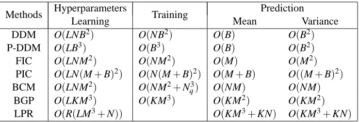
Methods Hyperparameters Training Prediction

Learning Mean Variance

DDM O(LNB2) O(NB2) O(B) O(B2) P-DDM O(LB3) O(B3) O(B) O(B2) FIC O(LNM2) O(NM2) O(M) O(M2) PIC O(LN(M+B)2_{) O(N(M+B)}2_{) O(M+B) O((M+B)}2₎ BCM O(LNM2_{) O(NM}2_+N3

q) O(NM) O(NM)

BGP O(LKM3) O(KM3) O(KM2) O(KM2) LPR O(R(LM3+N)) O(KM3+KN) O(KM3+KN)

Table 1: Comparison of computational complexities: we suppose that L iterations are required for learning hyperparameters; for DDM, the number of control points q on a boundary is kept to be a small constant as discussed in Remark 1; for BCM, Nq is the number of testing

points; for BGP, K is the number of bootstrap samples, M is the size of each bootstrap sample; for LPR, R is the number of the subsets of training points used for estimating local hyperparameters and K is the number of local experts of size M.

much slower than expected. The computational complexity of DDM is similar to FIC, as shown in Table 1. One way that can significantly improve the computation is through parallelization, which is easier to conduct for DDM because the m local predictions can be performed simultaneously. If a full parallelization can be done, the computational complexity for one iteration using DDM reduces to O(B3), where nj=B is assumed for all j’s. For more comparison results, see Table 1.

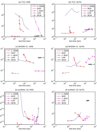
6. Experimental Results

In this section, we present some experimental results for evaluating the performance of DDM. First, we show how DDM works as the tuning parameters of DDM (p, q and m) change, and provide some guidance on setting the tuning parameters when applying DDM. Then, we compare DDM with several competing methods in terms of computation time and prediction accuracy. We also evaluate how well DDM can solve the problem of prediction mismatch on boundaries.

The competing methods are local GP (i.e., local kriging), FIC (Snelson and Ghahramani, 2006), PIC (Snelson and Ghahramani, 2006), BCM (Tresp, 2000), and LPR (Urtasun and Darrell, 2008). We also include in our comparative study the Bagged Gaussian Processes (BGP, Chen and Ren, 2009) as suggested by a referee, because it is another way to provide continuous prediction sur-faces by smoothly combining independent GPs. BGP was originally developed for improving the robustness of GP regression, not for the purpose of faster computation. The prediction by BGP is an average of the predictions obtained from multiple bootstrap resamples, each of which has the same size as the training data. Hence, its computational complexity is no better than the full GP regression. But faster computation can be achieved by reducing the bootstrap sample size to a small number M≪N, a strategy used in our comparison.

fairness. The remaining methods are designed to allow local hyperparameters, so DDM uses local hyperparameters for comparison with those.

We did not compare DDM with the the mixture of GP experts such as MGP (Rasmussen and Ghahramani, 2002) and TGP (Gramacy and Lee, 2008), because their computation times are far worse than the other compared methods especially for large data sets, due to the use of computa-tionally slow sampling methods. For example, according to our simple experiment, it took more than two hours for TGP to train its predictor for a data set with 1,000 training points and took more than three days (79 hours) for a larger data set with 2,000 training points, while other competing methods took only a few seconds. We did not directly implement and test MGP, but according to Gramacy and Lee (2008, page 1126), MGP’s computation efficiency is no better than TGP. In gen-eral, the sampling based approaches are not competitive for handling large-scale data sets and thus are inappropriate for comparison with DDM, even though they may be useful on small to medium-sized data sets in high dimension.

6.1 Data Sets and Evaluation Criteria

We considered four data sets: two synthetic data sets (one in 1-d and the other in 2-d) and two real spatial data sets both in 2-d. The synthetic data set in 1-d is packed together with the FIC implementation by Snelson and Ghahramani (2006). It consists of 200 training points and 301 test points. We use this synthetic data set to illustrate that PIC still encounters the prediction mismatch problem at boundaries, while the proposed DDM does solve the problem for 1-d data. The second synthetic data set in 2-d, synthetic-2d, was generated from a stationary GP with an isotropic squared exponential function using the R packageRandomFields, where nugget = 4, scale=4, and variance=8 are set as parameters for the covariance function. It consists of 63,001 sample points.

The first real data set, TCO, contains data collected by NIMBUS-7/TOMS satellite to measure the total column of ozone over the globe on Oct 1 1988. This set consists of 48,331 measurements. The second real data set,MOD08-CL, was collected by the Moderate Resolution Imaging Spectro-radiometer (MODIS) on NASA’s Terra satellite that measures the average of cloud fractions over the globe from January to September in 2009. It has 64,800 measurements. Spatial non-stationarity presents in both real data sets.

Using the second synthetic data set and the two real spatial data sets, we compare the computa-tion time and prediccomputa-tion accuracy among the competing methods. We randomly split each data set into a training set containing 90% of the total observations and a test set containing the remaining 10% of the observations. To compare the computational efficiency of methods, we measure two computation times, the training time (including the time for hyperparameter learning) and the pre-diction (or test) time. For comparison of accuracy, we use three measures on the set of the test data, denoted as{(xt,yt);t=1, . . . ,T}, where T is the total data amount in the test set. The first measure

is the mean squared error (MSE)

MSE= 1

T T

∑

t=1

(yt−µt)2,

which measures the accuracy of the mean prediction µtat location xt. The second one is the negative

log predictive density (NLPD)

NLPD= 1

T T

∑

t=1

(yt−µt)2

2σ2t

+1

2log(2πσ 2

t)

which considers the accuracy of the predictive varianceσt as well as the mean prediction µt. These

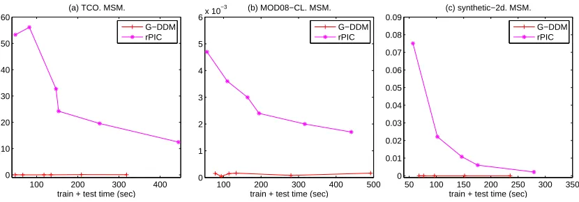
two criteria were used broadly in the GP regression literature. The last measure, the mean squared mismatch (MSM), measures the mismatches of mean prediction on boundaries. Given a set of test points, {xe; e=1, . . . ,E}, located on the boundary between subdomains Ωi andΩj, the MSM is

defined as

MSM= 1

E E

∑

e=1

(µ(ei)−µ(ej))2,

where µe(i) and µe(j) are mean predictions fromΩi andΩj, respectively. A smaller value of MSE,

NLPD or MSM indicates a better performance.

Our implementation of DDM was mostly done in MATLAB. When applying DDM to the 2-d spatial data, one issue is how to partition the whole domain into subdomains, also known as meshing in the finite element analysis literature (Ern and Guermond, 2004). A simple idea is just to use a uniform mesh, where each subdomain has roughly the same size. However simple, this idea works surprisingly well in many applications, including our three data sets in 2-d. Thus, we used a uniform mesh with each subdomain shaped rectangularly in our implementation.

For FIC, we used the MATLAB implementation by Snelson and Ghahramani (2006), while for BCM, the implementation by Schwaighofer et al. (2003) was used. Since the implementations of the other methods are not available, we wrote our own codes for PIC, LPR and BGP. Throughout the numerical analysis, we used the anisotropic version of a squared exponential covariance function. All numerical studies were performed on a computer with two 3.16 GHz quadcore CPUs.

6.2 Mismatch of Predictions on Boundaries

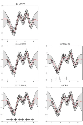
DDM puts continuity constraints on local GP regressors so that predictions from neighboring local GP regressors are the same on boundaries for 1-d data and are well controlled for 2-d data. In this section, we show empirically, by using the synthetic 1-d data set and the 2-d (real)TCOdata set, the effectiveness of having the continuity constraints.

For the synthetic data set, we split the whole domain,[−1,7], into four subdomains of equal size. The same subdomains are used for local GP, PIC and DDM. PIC is also affected by the number and locations of inducing inputs. To see how the mismatch of prediction is affected by the number of inducing inputs, we considered two choices, five and ten, as the number of inducing inputs for PIC. The locations of inducing inputs along with the hyperparameters are chosen by optimizing the marginal likelihood. For DDM, the local hyperparameters are obtained for each subdomain using the method described in Section 5.

Figure 1 shows for the synthetic data the predictive distributions of the full GP regression, local GP, PIC with M=5, PIC with M=10, and DDM. In the figure, red lines are the predictive means of the predictive distributions. The mean of local GP and the mean of PIC with M=5 have substantial discontinuities at x=1.5 and x=4.5, which correspond to the boundary points of subdomains. As M increases to 10, the discontinuities decrease remarkably but are still visible. In general, the mismatch in prediction on boundaries is partially resolved in PIC by increasing the number of inducing inputs at the expense of longer computing time. By contrast, the mean prediction of DDM is continuous, and close to that of the full GP regression.

0 2 4 6 −3

−2 −1 0 1 2

(a) full GPR

0 2 4 6

−3 −2 −1 0 1 2

(b) local GPR

0 2 4 6

−3 −2 −1 0 1 2

(c) PIC (M=5)

0 2 4 6

−3 −2 −1 0 1 2

(d) PIC (M=10)

0 2 4 6

−3 −2 −1 0 1 2

(e) DDM

0 2 4 6 8 10 12 0

1 2 3 4 5

(a) MSM (p=3)

# of control points (q)

0 2 4 6 8 10 12

0 1 2 3 4 5

(c) MSM (p=5)

# of control points (q)

0 2 4 6 8 10 12

0 1 2 3 4 5

(e) MSM (p=8)

# of control points (q)

0 2 4 6 8 10 12

10 12 14 16 18 20

(b) MSE (p=3)

# of control points (q)

0 2 4 6 8 10 12

10 12 14 16 18 20

(d) MSE (p=5)

# of control points (q)

0 2 4 6 8 10 12

10 12 14 16 18 20

(f) MSE (p=8)

# of control points (q)

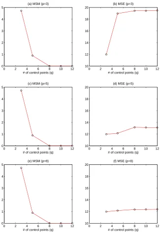
Figure 2: Left column: MSM versus the degrees of freedom p and the number of control points q; Right column: MSE versus p and q.

We observe from Figure 2 that for the TCO data set, the magnitude of prediction mismatch, measured by MSM, decreases as we increase the number of control points. We also observe that there is no need to use too many control points. For the 2-d data sets at hand, using more than eight control points does not help much in decreasing the MSM further; and the MSM is close to zero with eight (or more) control points. On the other hand, if the degrees of freedom (p) is small but the number of control points is larger, the MSE could increase remarkably (see Figure 2-(b)). This is not surprising, because the degrees of freedom determines the complexity of a boundary function, and if we pursue better match with too simple boundary function, we would distort local predictors a lot, which will in the end hurt the accuracy of the local predictors. If p is large enough to represent the complexity of boundary functions, the MSE stays roughly constant regardless of q (see Figure 2-(d) and 2-(f)). To save space, we do not present here the results for another real data set, MOD08-CL, because they are consistent with those for TCO. Our general recommendation is to use a reasonably large p and let q=p.

6.3 Choice of Mesh Size for DDM

An important tuning parameter in DDM is the mesh size. In this section, we provide a guideline for an appropriate choice of the mesh size through some designed experiments. The mesh size is defined by the number of training data points in a subdomain, previously denoted by B. We empirically measure, using the synthetic-2d,TCOandMOD08-CLdata sets, how MSE and training/testing times change for different B’s. In order to characterize the goodness of B, we introduce in the following a “marginal MSE loss” with respect to the total computation time Time, that is, training time + test time, measured in seconds. Given a set of mesh sizes

B

marginal(B; B∗):=max

0, MSE(B)−MSE(B

∗₎

1+Time(B∗)−Time(B)

for B∈

B

where B∗=max{B∈

B

B, while the numerator implies how much MSE we lost with the time saving. But marginal(B; B∗) alone is not a good enough measure because marginal(B; B∗) is always zero at B=B∗. So, we balanced the loss by adding the change in MSE and computation relative to the smallest mesh size in

B

marginal MSE loss :=marginal(B; B∗) +marginal(B; B◦),

where B◦=min{B∈

B

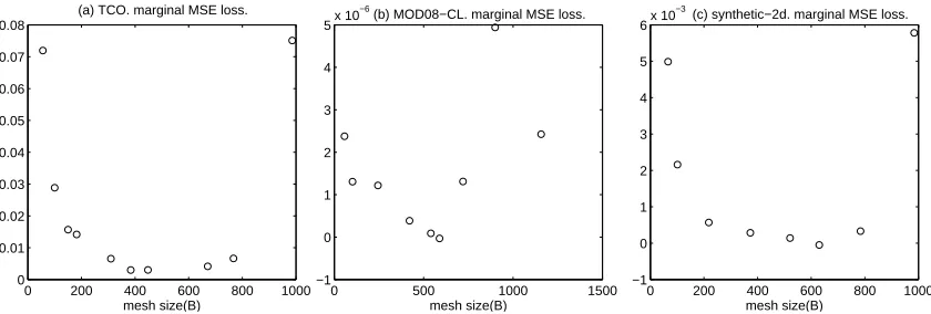
Figure 3 shows the marginal MSE loss for the three data sets. For all data sets, a B between 200 and 600 gives smaller marginal MSE loss. Based on this empirical evidence, we recommend to choose the mesh size so that the number of training data points in a subdomain ranges from 200 to 600. If the number is too large, DDM will spend too much time for small reduction of MSE. Conversely, if the number is too small, MSE will deteriorate significantly. The latter might be because DDM has too fewer training data points to learn local hyperparameters.

6.4 DDM Versus Local GP

hyperpa-0 200 400 600 800 1000 0

0.01 0.02 0.03 0.04 0.05 0.06 0.07 0.08

mesh size(B) (a) TCO. marginal MSE loss.

0 500 1000 1500

−1 0 1 2 3 4 5x 10

−6

mesh size(B)

(b) MOD08−CL. marginal MSE loss.

0 200 400 600 800 1000

−1 0 1 2 3 4 5 6x 10

−3

mesh size(B)

(c) synthetic−2d. marginal MSE loss.

Figure 3: Marginal MSE loss versus mesh size(B). For the three data sets, the marginal loss is small when B is in between 200 and 600.

rameters (G-DDM) and the other using local hyperparameters (L-DDM). For local GP, we always used local hyperparameters.

Figure 4 shows the three performance measures as a function of the number of subdomains for G-DDM, L-DDM and local GP, using theTCOdata and the synthetic-2d data, respectively. DDM adds more computation to local GP for imposing the continuity on boundaries, but the increased computation is very small relative to the original computation of local GP. Hence, the comparison of DDM with local GP as a function of the number of subdomains is almost equivalent to the comparison in terms of the total time (i.e., training plus test time).

In Figure 4, local GP has bigger MSE and NLPD than the two versions of DDM for both data sets. The better performance of DDM can be contributed to the better prediction accuracy around boundaries of subdomains. The comparison results for two versions of DDM are as expected: In terms of MSE and NLPD, L-DDM is better than G-DDM for theTCO data set, which can be explained by nonstationarity of the data. On the other hand, for the synthetic-2d data set, G-DDM is better, which is not surprising since the synthetic-2d data set is generated from a stationary GP so one would expect that global hyperparameters work well.

The left panels of Figure 5 show the comparison results for the actual MOD08-CLdata set. In terms of MSE and NLPD, L-DDM is appreciably better than local GP when the number of subdo-mains is small, but the two methods perform comparably when the number of subdosubdo-mains is large. This message is somewhat different from what we observed forTCOdata set. One explanation is that

TCOdata set has several big empty spots with no observation over the subregion, butMOD08-CLdata set does not have such “holes”. Because of the continuity constrains, we believe DDM is able to borrow information from neighboring subdomains, and consequently, to provide better spatial pre-dictions. To verify this, we randomly chose twenty locations within the spatial domain ofMOD08-CL

data set and artificially removed small neighborhoods of each randomly chosen location from the

MOD08-CLdata set; doing so resulted in a new data set called “MOD08-CLwith holes”. The results of applying three methods on this new data set are shown on the right panels of Figure 5. L-DDM is clearly superior over local GP across different choices of the number of subdomains.

the prediction accuracy. More importantly, the improvement in prediction can be further enhanced by a proper effort to smooth out the boundary mismatches in localized methods (L-DDM versus local GP). In all cases, the MSM associated with DDM method is very small.

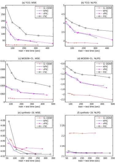
6.5 G-DDM Versus FIC and PIC

We compared prediction accuracy of G-DDM with FIC and PIC. We only considered global hyper-parameters for DDM because FIC and PIC cannot incorporate local hyperhyper-parameters. Since each of the compared methods has different tuning parameters, it is hard to compare these methods using prediction accuracy measures (MSE and NLPD) for a fixed set of tunning parameters. Instead, we considered MSE and NLPD as a function of the total computation time required. To obtain the prediction accuracy measures for different computation times, we tried several different settings of experiments and presented the best accuracies of each method for given computation times: for DDM, we varied the number of equally sized subdomains (m) and the number of control points

q while keeping the degrees of freedom p the same as q; we tested two versions of PIC having

different domain decomposition schemes: k-means clustering (denoted by kPIC) and regular grids meshing (denoted by rPIC), and for each version, we varied the total number of subdomains (m) and the number of inducing inputs (M); for FIC, we varied the number of inducing inputs (M). We see that each of the compared methods has one major tuning parameter mainly affecting their training and test times; it is m for DDM, or M for FIC and PIC. In order to obtain one point in Figure 6, we first fixed the major tuning parameter for each method, and then changed the remaining parameters to get the best accuracy for a given computation time.

In this empirical study, for G-DDM, a set of the global hyperparameters was learned by mimizing (23). In FIC, the global hyperparameters, together with the locations of the inducing in-puts, were determined by maximizing its marginal likelihood function. For PIC, we tested several options: learning the hyperparameters and inducing inputs by maximizing the PIC approximated marginal likelihood; learning the hyperparameters by maximizing the PIC approximated marginal likelihood, whereas learning the inducing inputs by the FIC approximated likelihood; or learning the hyperparameters by the FIC approximated marginal likelihood, whereas learning the inducing inputs by the PIC approximated marginal likelihood. Theoretically, the first option should be the best choice. However, as discussed in Section 5, due to the non-linear and non-convex nature of the likelihood function, an optimization algorithm may converge to a local optimum and thus yields a suboptimal solution. Consequently, it is not clear which option’s local optimum produces the best performance. According to our empirical studies, for theTCOdata set, the first option gave the best result, while for theMOD08-CLdata set, the third option was the best. We present the results based on the empirically best result.

0 100 200 300 400 500 12 14 16 18 20 22 24

# of subdomains (a) TCO. MSE.

0 100 200 300 400 500 600 4 4.05 4.1 4.15 4.2 4.25

# of subdomains (b) synthetic−2d. MSE.

0 100 200 300 400 500 2.7 2.75 2.8 2.85 2.9 2.95 3

# of subdomains (c) TCO. NLPD.

0 100 200 300 400 500 600 2.21 2.215 2.22 2.225

# of subdomains (d) synthetic−2d. NLPD.

0 100 200 300 400 500 0 5 10 15 20

# of subdomains (e) TCO. MSM.

0 100 200 300 400 500 600 −0.1 0 0.1 0.2 0.3 0.4 0.5

# of subdomains (f) synthetic−2d. MSM. G−DDM L−DDM local GP G−DDM L−DDM local GP G−DDM L−DDM local GP G−DDM L−DDM local GP G−DDM L−DDM local GP G−DDM L−DDM local GP

0 100 200 300 400 500 600 6 8 10 12

x 10−4

# of subdomains (a) MOD08−CL. MSE.

0 100 200 300 400 500 600 6 8 10 12

x 10−4

# of subdomains (b) MOD08−CL with holes. MSE.

0 100 200 300 400 500 600 −2.5 −2.4 −2.3 −2.2 −2.1 −2 −1.9 −1.8 −1.7

# of subdomains (c) MOD08−CL. NLPD.

0 100 200 300 400 500 600 −2.5 −2.4 −2.3 −2.2 −2.1 −2 −1.9 −1.8 −1.7

# of subdomains (d) MOD08−CL with holes. NLPD.

0 100 200 300 400 500 600 0 0.5 1 1.5 2 2.5

x 10−3

# of subdomains (e) MOD08−CL. MSM.

0 100 200 300 400 500 600 0 0.5 1 1.5 2 2.5

x 10−3

# of subdomains (f) MOD08−CL with holes. MSM. G−DDM L−DDM local GP G−DDM L−DDM local GP G−DDM L−DDM local GP G−DDM L−DDM local GP G−DDM L−DDM local GP G−DDM L−DDM local GP