Assessing Approximate Inference for Binary Gaussian Process Classification

Assessing Approximate Inference for

Binary Gaussian Process Classification

Malte Kuss [email protected]

Carl Edward Rasmussen [email protected]

Max Planck Institute for Biological Cybernetics Spemannstraße 38

72076 T¨ubingen, Germany

Editor: Ralf Herbrich

Abstract

Gaussian process priors can be used to define flexible, probabilistic classification models. Unfor-tunately exact Bayesian inference is analytically intractable and various approximation techniques have been proposed. In this work we review and compare Laplace’s method and Expectation Prop-agation for approximate Bayesian inference in the binary Gaussian process classification model. We present a comprehensive comparison of the approximations, their predictive performance and marginal likelihood estimates to results obtained by MCMC sampling. We explain theoretically and corroborate empirically the advantages of Expectation Propagation compared to Laplace’s method.

Keywords: Gaussian process priors, probabilistic classification, Laplace’s approximation,

expec-tation propagation, marginal likelihood, evidence, MCMC

1. Introduction

In recent years models based on Gaussian process (GP) priors have attracted much attention in the machine learning community. Whereas inference in the GP regression model with Gaussian noise can be done analytically, probabilistic classification using GPs is analytically intractable, see Ras-mussen and Williams (2006) for a general overview. Several approaches to approximate Bayesian inference have been suggested, including Laplace’s method, Expectation Propagation (EP), varia-tional approximations and Markov chain Monte Carlo (MCMC) sampling, some of these in con-junction with generalisation bounds, online learning schemes and sparse approximations (e.g. Neal, 1998; Williams and Barber, 1998; Gibbs and MacKay, 2000; Opper and Winther, 2000; Csat´o and Opper, 2002; Seeger, 2002; Lawrence et al., 2003).

Despite the abundance of recent work on probabilistic GP classifiers, most experimental studies provide only anecdotal evidence, and no clear picture has yet emerged, as to when and why which algorithm should be preferred. Thus, from a practitioners point of view it is unclear what the method of choice is for probabilistic GP classification. In this work, we set out to understand and compare two of the most wide-spread approximations: Laplace’s method and Expectation Propagation (EP). We also compare to a sophisticated, but computationally demanding MCMC scheme, which be-comes exact in the limit of long running times. We do not address issues of sparsification but stick to comparing the two types of approximation.

In any practical application of GPs in classification (usually multiple) parameters of the covariance function (hyper-parameters) have to be handled. Bayesian model selection provides a consistent framework for setting such parameters. Therefore, it is essential to evaluate the accuracy of the marginal likelihood approximations as a function of the hyper-parameters, in order to assess the practical usefulness of the approach. The related question of whether the marginal likelihood cor-relates well with the generalisation performance cannot be answered in general but depends on the appropriateness of the model for a given data set. However, we do assess this empirically for two data sets.

Secondly, we need to assess the quality of the approximate probabilistic predictions. In the past, the probabilistic nature of the GP predictions has not received much attention, the focus being mostly on classification error rates. This unfortunate state of affairs is caused primarily by typical benchmarking problems being considered outside of a realistic context. The ability of a classifier to produce class probabilities or confidences, have obvious relevance in most areas of application, e.g. medical diagnosis and ROC analysis. We evaluate the predictive distributions of the approxi-mate methods, and compare to the MCMC gold standard.

2. The Gaussian Process Model for Binary Classification

In this section we describe the Gaussian process model for binary classification (GPC). Let y_∈ {−1,1_}denote the class label corresponding to an input x. The GPC model is discriminative in the sense that it models p(y_|x)which for fixed x is a Bernoulli distribution. The probability of success

p(y=1_|x)is related to an unconstrained latent function f(x)which is mapped to the unit interval by a sigmoidal transformation, e.g. the logit or the probit. Both mappings are relatively similar around zero but show different tail behaviour. We will not examine the difference in this study. For reasons of analytic convenience (for the EP algorithm) we exclusively use the probit model

p(y=1_|x) =Φ(f(x)), where Φ denotes the cumulative density function of the standard normal distribution.

In the GPC model Bayesian inference is performed about the latent function f in the light of observed data

D

=_{(yi,xi)|i=1, . . . ,m}. Let fi= f(xi)and f= [f1, . . . ,fm]>be shorthand for the values of the latent function and y= [y1, . . . ,ym]>and X= [x1, . . . ,xm]>collect the class labels and inputs respectively.

Given the latent function, the class labels are independent Bernoulli variables, so the joint like-lihood factorises:

p(y_|f) =

m

∏

i=1

p(yi|fi) (1)

and depends on f only through its value at the corresponding observed inputs. For the probit model the individual likelihood terms become p(yi|fi) =Φ(yifi), due to the symmetry ofΦ.

As prior over functions f we use a zero-mean Gaussian process (GP) prior (O’Hagan, 1978). A GP is a stochastic process where each input x has an associated random variable f(x). The joint distribution of function values corresponding to any set of inputs X is multivariate Gaussian

p(f_|X,θ) =

N

(f_|0_{,K). The covariance matrix is defined element-wise, Ki j =k(xi,xj,θ) where k}

is a positive definite covariance function parameterised byθ. Note that by choosing a covariance function we introduce hyper-parameters θ to the prior. The zero-mean GP prior encodes that a

For details on covariance functions and their implications on the prior over functions see for example Abrahamsen (1997) or Rasmussen and Williams (2006, ch. 4).

Using Bayes’ rule the posterior distribution over the latent function values f for given hyper-parametersθbecomes:

p(f_|

D

,θ) = p(y|f)p(f|X,θ) p(

D

_|θ) =

N

(f_|0_,K) p(

D

_|θ)

m

∏

i=1

Φ(yifi) (2)

which is non-Gaussian. Properties of the posterior will be described in Section 5.

The main purpose of classification models is to predict the class label y_∗for test inputs x_∗. The distribution of the latent function value can be computed by marginalisation:

p(f_∗|

D

,θ,x_∗) = Z

p(f_∗|f,X,θ,x_∗)p(f_|

D

,θ)df, (3)

and by computing the expectation:

p(y_∗|

D

,θ,x_∗) = Z

p(y_∗|f_∗)p(f_∗|

D

,θ,x_∗)d f_∗ (4)

the predictive distribution is obtained, which is again a Bernoulli distribution. The first term in the right hand side of equation (3) is Gaussian and obtained by conditioning the joint Gaussian prior distribution.

Unfortunately, neither the posterior eq. (2) p(f_|

D

,θ), the predictive distribution eq. (4) p(y_∗=

1_|

D

,θ,x_∗)nor the marginal likelihood eq. (7) p(

D

_|θ)can be computed analytically, so approxima-tions are needed. For the GPC model approximaapproxima-tions are either based on a Gaussian approximation

q(f_|

D

,θ) =

N

(f_|m,A)to the posterior p(f_|

D

,θ)or involve Markov chain Monte Carlo (MCMC) sampling.

A key insight is that a Gaussian approximation to the posterior implies a GP approximation to the posterior process, which gives rise to an approximate predictive distribution for test cases. Intro-ducing the approximate Gaussian posterior into eq. (3) gives the approximate posterior q(f_∗|

D

,θ,x_∗) =

N

(f_∗|µ_∗,σ2

∗), with mean and variance:

µ_∗ = k>_∗K−1m (5a)

σ2

∗ = k(x∗,x∗)−k>∗(K−1−K−1AK−1)k∗, (5b)

where k_∗= [k(x1,x_∗), . . . ,k(xm,x_∗)]> is a vector of prior covariances between x_∗and the training inputs X. For the probit likelihood the approximate predictive probability (4) of x_∗ belonging to class 1 can be computed analytically:

q(y_∗=1_|

D

,θ,x_∗) = Z

Φ(f_∗)

N

(f_∗|µ_∗,σ2

∗)d f∗=Φ

µ

∗ √

1+σ2

∗

. (6)

The parameters m and A of the posterior approximation can be found using Laplace’s method (Section 3) or by Expectation Propagation (Section 4).

However, a model selection approach can be implemented by selectingθmaximising the marginal likelihood (evidence):

p(

D

_|θ) = Z

p(y_|f)p(f_|X,θ)df (7) which can be understood as a measure of the agreement between the model and observed data (Kass and Raftery, 1995; MacKay, 1999). This approach is called maximum likelihood II (ML-II) type hyper-parameter estimation and motivates the need for computing the marginal likelihood. Laplace’s method as well as Expectation Propagation provide an approximation to the marginal likelihood (7) and so approximate ML-II hyper-parameter estimation can be implemented in both approximation schemes.

3. Laplace’s Method

Williams and Barber (1998) describe Laplace’s method to find a Gaussian

N

(f_|m,A)approximation to the posterior over latent function values (2) for fixedθ(although they use the logit likelihood). Let ln

L

(f) = ln p(y_|f)denote the log likelihood and:

ln

Q

(f_|

D

,θ) =ln

L

(f)₋1

2ln|K| − 1 2f

>_K−1_f

−m₂ ln(2π) (8)

the unnormalised log posterior. Laplace’s approximation is found by a second order Taylor expan-sion:

ln

Q

(f_|

D

,θ)_'ln

Q

(m)₋1

2(m−f)

>_A−1_(m

−f) (9)

around the mode of the (log) posterior:

m=argmax f∈Rm

ln

Q

(f_|

D

,θ). (10)

Since both the likelihood and the prior are log-concave the posterior is also log-concave and uni-modal. Let:

∇fln

Q

= ∇fln

L

(f)−K−1f (11a)

∇∇fln

Q

= ∇∇fln

L

(f)−K−1 (11b)

denote the gradient and the Hessian. The mode is conveniently found using Newton’s method, iterating:

f _← f₋(∇∇fln

Q

(f))−1∇fln

Q

(f), (12) which usually converges rapidly to m. The covariance matrix:

A = ₋ ∇∇fln

Q

(m) −1

= (K−1+W)−1 (13)

is approximated by the curvature at the mode, equal to the negative inverse Hessian, where W=

−∇∇fln

L

.

This approximation also facilitates an approximation to the marginal likelihood:

p(

D

_|θ) = Z

p(y_|f)p(f_|X,θ)df = Z

Algorithm 1 Laplace’s approximation for GPC Given:θ,

D

, x_∗

Initialise f (e.g. f_←0_{), compute K fromθand X} repeat

f←f−(∇∇fln

Q

(f))−1∇fln

Q

(f) until convergence of f

m_←f

A←(K−1₋∇∇

fln

Q

(m))−1

Compute log marginal likelihood ln q(

D

_|θ)by (15), and predictions q(y_∗=1_|

D

,θ,x_∗)using (6).

Substituting ln

Q

by its Taylor approximation (9) the Gaussian integral can be solved. The resulting approximate log marginal likelihood is:

ln p(

D

_|θ) _' ln q(

D

_|θ) = ln

Q

(m) +m

2 ln(2π) + 1

2ln|A| (15)

and the derivative of this quantity w.r.t.θcan be derived and used for optimisation (e.g. using conju-gate gradient methods) in an ML-II type setting. See Algorithm 1 for an overview and Appendix A for details about our implementation.

4. Expectation Propagation

Minka (2001) proposed the iterative Expectation Propagation (EP) algorithm which can by applied to GPC. EP finds a Gaussian approximation q(f_|

D

,θ) =

N

(f_|m,A) to the posterior p(f_|

D

,θ) by moment matching of approximate marginal distributions. The starting point is an approximation mimicking the factorising structure:

p(f_|

D

,θ) = p(f|X,θ) p(

D

_|θ)

m

∏

i=1

p(yi|fi) '

p(f_|X,θ) q(

D

_|θ)

m

∏

i=1

t(fi,µi,σ2_i,Zi) = q(f|

D

,θ), (16) where throughout we use p to denote exact quantities and q approximations, and the terms:

t(fi,µi,σ2_i,Zi) = Zi

N

(fi|µi,σ2i) (17) are called site functions. Note that the site functions are approximating the likelihood (which nor-malizes over observations yi), with a Gaussian in fi, so we cannot expect the site functions to normalize, hence the explicit term Zi is necessary. For notational convenience we hide the site

pa-rameters µi,σ2i and Ziand write t(fi)instead. From (17) the Gaussian approximation (16) has mean and covariance:

q(f_|

D

,θ) =

N

(f_|m,A), where m = AΣ−1_{µ, and A = (K}−1₊Σ−1₎−1_{, (18)}

whereµ= (µ1, . . . ,µm)>andΣ=diag(σ21, . . . ,σ2m)collect site function parameters. The EP algo-rithm iteratively visits each site function in turn, and adjusts the site parameters to match moments of an approximation to the posterior marginals. The kth moment of fiunder the posterior is:

hf_ik_i = 1

p(

D

_|θ) Z

f_ikp(y_|f)p(f_|X,θ)df = 1 p(

D

_|θ)

Z

where:

p\i(fi) =

Z

∏

j6=i

p(yj|fj)p(f|X,θ)df\i (20)

is called the cavity distribution and f\i_{denotes f without f}

i. The marginalisation required to compute the exact cavity distribution is intractable for the GPC model. The key step in the EP algorithm is to replace the intractable exact cavity distribution with a tractable approximation based on the site functions:

q\i(fi) =

Z

∏

j6=i

t(fj)p(f|X,θ)df\i. (21)

The approximate cavity function comes in the form of an unnormalised Gaussian q\i(fi)∝

N

(fi|µ\i,σ2_\i).

Multiplying both sides by t(fi):

q\i(fi)t(fi) =

Z

N

(f_|0,K)

m

∏

j=1

t(fj)df\i ∝

N

(fi|mi,Aii), (22)

and basic Gaussian identities give the parameters:

σ2

\i= (Aii)−

1

−σ−i 2

−1

and µ\i=σ2_\i

mi

Aii−

µi

σ2

i

, (23)

of the approximate cavity function.

The core idea of EP is to adjust the site parameters µi,σiand Ziso that the approximate posterior marginal using the exact likelihood approximates as well as possible the posterior marginal based on the site function:

q\i(fi)p(yi|fi) ' q\i(fi)t(fi,µi,σ2i,Zi) (24) by matching the zeroth, first and second moments. Recall that matching of moments minimizes Kullback-Leibler (KL) divergence.1 For the probit likelihood p(y_i|fi) =Φ(yifi)the k=0,1,2 mo-ments of the left hand side can be computed analytically

m0 = Φ

yµ

\i

√ 1+σ2

\i

= Φ(z), (25a)

m1 = µ\i+

σ2

\i

N

(z|0,1)

Φ(z)y√1+σ2

\i

, (25b)

m2 = 2µ\im1−µ2\i+σ

2

\i−

zσ4_\i

N

(z|0,1)

Φ(z)(1+σ2

\i)

, (25c)

where z=yµ\i/

√ 1+σ2

\i. By equating these moments with those of the right hand side of (24) the

update equations for the site parameters become

σ2

i = (m2−m21)−1−σ−\i2

−1

, (26a)

µi = σ2i

m1(σ−\i2+σ−

2

i )−

µ\i

σ2

\i

, (26b)

Zi = m0

q

2π(σ2_\i+σ2i)exp

(µi−µ\i)2

2(σ2_\i+σ2i) !

. (26c)

Algorithm 2 EP for Gaussian process classification Given:θ,

D

, x_∗

Initialise: A_←K and site parametersσ2_i and µi

repeat

for i=1,. . . ,m do

Compute parameters (23) of cavity Compute moments (25)

Update the site parameters using (26) Update m and A according to (18)

end for

until The site parameters converged

Compute log marginal likelihood ln q(

D

_|θ)by (27), and predictions q(y_∗=1_|

D

,θ,x_∗)using (6).

In the application of EP, one may generally not have a guarantee that the new site variance in (26a) is non-negative; however, in the GPC model with probit likelihood, one can show that variance is always positive. Once we have new values for µi andσ2i we have to update m and A according to (18), which in practise is done using rank-one updates, to save computation.

The EP algorithm iteratively updates the site parameters as shown in Algorithm 2. Although we cannot prove the convergence of EP, we conjecture that it always converges for GPC with probit likelihood, and have never encountered an exception.

Finally the approximate log marginal likelihood can be obtained from the normalization of (16), giving

ln p(

D

_|θ) _' ln q(

D

_|θ) = ln

Z

q(f_|X,θ)

m

∏

i=1

t(fi)df (27)

=

n

∑

i=1

ln Zi− 1

2ln|K+Σ| − 1 2µ

>_(K+Σ₎−1_µ−m

2 ln(2π).

Perhaps this is not the standard way to compute an approximation to the marginal likelihood used elsewhere, but it seems the most natural given the approximation. The derivatives of the log marginal likelihood can be computed in order to implement ML-II parameter estimation ofθ. Algorithm 2 summarises the computations, more details on implementing EP for GPC can be found in Ap-pendix B.

5. Structural Properties of the Posterior

In the previous sections we described the GPC model and two alternative approximation schemes for finding a Gaussian approximation to the posterior. This section provides more details on the properties of the posterior which is compared to the structure of the respective approximations.

Figure 1(a) provides a one-dimensional illustration. The prior

N

(f_|0,52_{) combined with the}

probit likelihood (y=1) results in a skewed posterior. Intuitively, the likelihood cuts off the f values which have the opposite sign of y. The mode of the posterior remains relatively close to the origin, while the mass is placed over positive values in accordance with the observation. Laplace’s approximation peaks at the posterior mode, but places far too much mass over negative values of

−40 0 4 8 0.02

0.04 0.06 0.08 0.1 0.12 0.14 0.16

p(f|y)

−4 0 4 8 0

0.2 0.4 0.6 0.8 1

f

p(y|f)

Likelihood p(y|f) Prior p(f) Posterior p(f|y) Laplace q(f|y) EP q(f|y)

(a) (b)

Figure 1: Panel (a) provides a one-dimensional illustration of approximations. The prior

N

(f_|0,52)

combined with the probit likelihood(y=1)results in a skewed posterior. The likelihood uses the right axis, all other curves use the left axis. In Panel (b) we caricature a high dimensional zero-mean Gaussian prior as an ellipse. The gray shadow indicates that for a high dimension Gaussian most of the mass lies in a thin shell. For large latent signals, the likelihood essentially cuts off regions which are incompatible with the training labels (hatched area), leaving the upper right orthant as the posterior. The dot represents the mode of the posterior, which is relatively unaffected by the truncation and remains close to the origin.

posterior moments, which results in a larger mean and a more accurate placement of probability mass compared to Laplace’s approximation.

Structural properties of the posterior in higher dimensions can best be understood by examining its construction. The prior is a correlated m-dimensional Gaussian

N

(f_|0_{,K)centred at the origin.}

Each likelihood term p(y_i|fi)softly truncates the half-space from the prior that is incompatible with the observed label, see Figure 1(b). The resulting posterior is unimodal and skewed, similar to a multivariate Gaussian truncated to the orthant containing y. The mode of the posterior remains close to the origin, while the mass is placed in accordance with the observed class labels. Addi-tionally, high dimensional Gaussian distributions exhibit the property that most probability mass is contained in a thin ellipsoidal shell—depending on the covariance structure—away from the mean (MacKay, 2003, ch. 29.2). Intuitively this occurs since in high dimensions the volume grows ex-tremely rapidly with the radius. As an effect the mode becomes less representative (typical) for the prior distribution as the dimension increases. For the GPC posterior this property persists: the mode of the posterior distribution stays relatively close to the origin, still being unrepresentative for the posterior distribution, while the mean moves to the mass of the posterior making mean and mode differ significantly.

0 1

2

3 0 0.5

1 1.5

2 2.5

3

0

x

2

x₁

p(x

1

,x2

)

0 1 2 3

x₁

p(x

1

)

0 2 4 6

0 0.05 0.1 0.15 0.2 0.25 0.3 0.35 0.4 0.45

x i

p(x

i

)

(a) (b) (c)

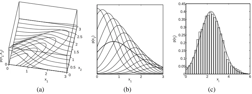
Figure 2: Panel (a) illustrates a bivariate normal distribution truncated to the positive quadrant. The lines describe slices through the probability density function for fixed x2-values. Panel (b)

shows the marginal distribution of p(x1)(thick line) obtained by (numerical) integration over x2, which—intuitively speaking—corresponds to an averaging of the slices (thin

lines) from Panel (a). Panel (c) shows a histogram of samples of a marginal distribution of an high-dimensional truncated Gaussian. The line describes a Gaussian with mean and variance estimated from the samples.

to the origin, such that the approximation will overlap with regions having practically zero posterior mass. As an effect the amplitude of the approximate latent posterior GP will be underestimated systematically, leading to overly cautious predictive distributions.

The EP approximation does not rely on a local expansion, but assumes that the marginal distri-butions of the posterior can be well approximated by Gaussians. As described above the posterior is similar to a high dimensional multivariate normal distribution truncated to one orthant. Although the posterior is skew and truncated, marginals of such a distribution can be relatively similar to a Gaussian.

As a low dimensional illustration the marginal distribution of a bivariate normal is shown in Figure 2(a-b). Depending on the covariance structure, the mode of the marginal distribution moves away from the origin and the distribution appear similar to a truncated univariate Gaussian.

In order to inspect the marginals of a truncated high-dimensional multivariate normal distri-bution we made an additional synthetic experiment. We constructed a 767 dimensional Gaussian

N

(x_|0_{,C)with a covariance matrix having one eigenvalue of 100 with eigenvector}1_{, and all other}

eigenvalues are 1. We then truncate this distribution such that all xi ≥0. Note that the mode of the truncated Gaussian is still at zero, whereas the mean moved towards the remaining mass. Metropolis-Hastings sampling was used to generate samples from this truncated multivariate distri-bution. Figure 2(c) shows a normalised histogram of samples from a marginal distribution of one

xi. The samples agree very well with a Gaussian approximation. Note that Laplace’s method would be completely inappropriate for approximating a truncated multivariate normal distribution.

6. Markov Chain Monte Carlo

Markov chain Monte Carlo (MCMC) may be too slow for many practical applications, but has the advantage that it becomes exact in the limit of long runs. Thus, MCMC can provide a gold standard by which to measure the two analytic methods of the previous sections. Computing the predictions via an MCMC estimate of (3) and (4) is relatively straight forward and covered in Section 6.1.

Good MCMC estimates of the marginal likelihood are, however, notoriously difficult to obtain, being equivalent to the free-energy estimation problem in physics (Gelman and Meng, 1998). In Section 6.2 we explain the use of Annealed Importance Sampling (AIS), which can be seen as a sophisticated elaboration of Thermodynamic Integration, for this task.

6.1 Hybrid MCMC Sampling

Hybrid Monte Carlo (HMC) sampling as proposed by Duane et al. (1987) is a computationally efficient sampling technique which exploits gradient information of the target distribution. Detailed accounts are given by Neal (1993, ch. 5.2) and Liu (2001, ch. 9). MacKay (2003, ch. 30) also provides pseudo-code; we do not repeat the details here.

HMC can be used to generate samples from the posterior p(f_|θ,

D

), while only the unnormalised log posterior (8) and its derivatives are required. As described in the previous section, the exact posterior (2) takes the form of a (correlated) Gaussian (the GP prior), which is (softly) truncated by the constraints imposed by the training labels through the likelihood. To ease the sampling task by reducing correlations, we first do a linear transformation into new g=L−1f variables, such that g is white w.r.t. K, where K=LL> is the Cholesky decomposition. Given samples from the posterior, we generate test-latents from the Gaussian p(f_∗|f,X,θ,x_∗)for use in a simple Monte Carlo estimate of (4).

6.2 Annealed Importance Sampling

The marginal likelihood (7) comes in the form of an m dimensional integral where m is the number of data points. A simple approach would be to use importance sampling with the EP or Laplace’s approximation of the posterior as proposal distribution. However, for the GPC model the resulting importance weights show enormous variances, making simple importance sampling useless for this task (MacKay, 2003, ch. 29).

Neal (2001) describes Annealed Importance Sampling (AIS), which we will use to estimate the marginal likelihood in the GPC model. Instead of solving the integral (7) directly, a sequence of easier quantities is computed. We define:

Zt =

Z

p(y_|f)τ(t)p(f_|X,θ)df (28)

where τ(t) is an inverse temperature schedule such that τ(0) =0 and τ(T) =1. The trick is to rewrite the marginal likelihood Z=p(

D

_|θ)as a fraction and expand:

Z = ZT Z0

= ZT

ZT₋1 ZT−1 ZT₋2···

Z1 Z0

Algorithm 3 Annealed Importance Sampling

Given: Temperature scheduleτ

for r=1, . . . ,R do

Sample f0from the prior

N

(f|0,K) for t=1, . . . ,T do

Sample ft from q(f|

D

,τ(t),θ)by HMC Compute ln(Zt/Zt−1)using (31) end for

Compute Zrusing (32)

end for

Return ln Z=ln _R1∑R_r=1Zr

where Z0 =1 since the prior normalises. Each term in (29) is approximated using importance

sampling using samples from q(f_|

D

,θ,τ(t))∝p(y_|f)τ(t)_p(f|X,θ): Zt

Zt−1 =

Z _p(y|f)τ(t)_p(f|_X,θ)

p(y_|f)τ(t−1)_p(f|X,θ)q(f|

D

,θ,τ(t−1))df (30a)

' 1

S

S

∑

i=1

p(y_|fi)τ(t)−τ(t−1) (30b)

where fi are samples from q(f|

D

,θ,τ(t)), which we generate using HMC. Using a single sample

S=1 and a large number of temperatures, the log of each ratio is:

ln(Zt/Zt₋1) ' τ(t)−τ(t−1)

ln p(y_|ft) (31)

where ft is the only sample at temperatureτ(t). Combining (29) with (31) we obtain the desired:

ln Z_' T

∑

t=1

ln(Zt/Zt−1). (32)

In all our experiments we useτ(t) = (t/T)4 _{for t=0, . . . ,8000. Using this temperature schedule}

we found that the sampling spends most of its efforts at temperatures with high variance of (31) such that the variance of (32) is relatively small. Note that this was only examined on the data sets we use below and only for certain values of θ. So far, we have described Thermodynamic Integration, which gives an unbiased estimate in the limit of slow temperature changes. In AIS the bias caused by finite temperature schedules is removed by combining multiple estimates by their geometric mean (see Algorithm 3). In the experiments we combine the estimates of R=3 runs of Thermodynamic Integration.

7. Experiments

In this section we compare and inspect approximations for GPC using various benchmark data sets. The primary focus is not to optimise the absolute performance of GPC models but to compare the relative accuracy of approximations and to validate the arguments given in Section 5.

In all the GPC experiments we use a covariance function of the form:

k(x,x0,θ) =σ2exp ₋₂1_`2 x−x0

2

−8 −6 −4 −2 0 2 4 0

0.2 0.4 0.6 0.8 1

x

p(y = 1|x)

Class 1 Class −1 Laplace p(y|X) EP p(y|X) True p(y|X)

(a)

−8 −6 −4 −2 0 2 4

−10 −5 0 5 10 15

x

f(x)

Laplace p(f|X) EP p(f|X)

(b)

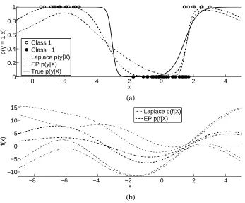
Figure 3: Synthetic classification problem: Panel (a) illustrates the classification task, the gen-erating p(y_|x) and two approximations thereof obtained by Laplace’s method and EP. Panel (b) illustrates the approximate predictive distributions p(f_∗|

D

,θ,x_∗) _'

N

(f_∗|µ_∗,σ2

∗)of latent function values showing the mean µ∗and the range of±2σ∗.

such that θ = [σ, `]. We refer to σ2 as the signal variance and to ` as the characteristic length-scale. Note that for many classification tasks it may be reasonable to use an individual length scale parameter for every input dimension (ARD). Nevertheless, for the sake of presentability we use the above covariance function and we believe the conclusions to be independent of this choice.

Both analytic approximations have a computational complexity which is cubic

O

(m3)as com-mon acom-mong non-sparse GP models due to inversions m_×m matrices. In our implementations

Laplace’s method and EP need similar running times, on the order of a few minutes for several hundred data-points. Making AIS work efficiently requires some fine-tuning and a single estimate of p(

D

_|θ)can take several hours for data sets of a few hundred examples, but this could conceivably be improved upon.

7.1 Synthetic Classification Problem

We computed Laplace’s and the EP approximation for the ML-II estimated value ofθthat max-imised Laplace’s approximation to the marginal likelihood (15). Note that this particular choice ofθ

should be in favour of Laplace’s method. Figure 3 shows the resulting classifiers and the underlying latent functions. In Figure 3(a) the approximations to p(y|x)appear to be similar for positive x but we observe an appreciable discrepancy for negative values. Laplace’s approximation gives an un-reasonably high predictive uncertainty, which is caused by a significant overlap of the approximate predictive distribution p(f_∗|

D

,θ,x_∗)_'

N

(f_∗|µ_∗,σ2

∗)with zero as shown in Figure 3(b). However,

note that both approximations agree on the sign of the predictive mean.

7.2 Ionosphere Data

The data consists of 351 examples in 34 dimensions. We standardised the inputs X to zero mean and unit variance. The training set is a random subset of size m=200 leaving the remaining 151 instances out as a test set.

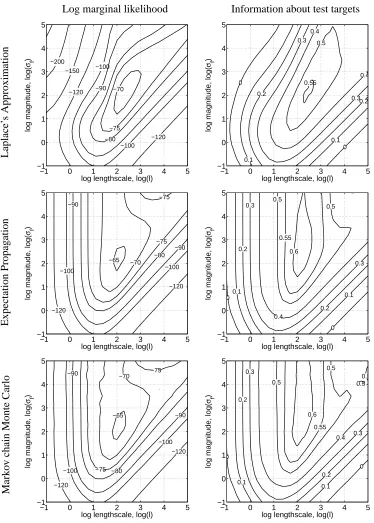
We do an exhaustive investigation on a regular 21_×21 grid of values for the log hyper-parameters. For eachθon the grid we compute the approximated log marginal likelihood by Laplace’s method (15), EP (27) and AIS. Additionally we compute the predictive performance on the test set. As performance measure we use the average information in bits of the predictions about the test targets in excess of that of random guessing. Let p∗=p(y_∗=1_|x_∗) be the model’s prediction, then we average:

I(p∗_i,yi) =yi+₂1log2(p∗i) +

1−yi

2 log2(1−p∗i) +H (34) over all test cases, where H is the entropy of the training set labels. Results are shown in Figure 4.

For all three approximation techniques we see an agreement between marginal likelihood esti-mates and test performance, which justifies the use of ML-II parameter estimation. But the shape of the contours and the values differ between the methods. The contours for Laplace’s method appear to be slanted compared to EP. The estimated marginal likelihood estimates of EP and AIS agree very well.2 The EP predictions contain as much information about the test cases as the MCMC predictions and significantly more than for Laplace’s method.

Note that for small signal variances (roughly ln(σ2)<0) Laplace’s method and EP give very similar results. A possible explanation is that for small signal variances the likelihood does not

truncate the prior but only down-weights the tail that disagrees with the observation. As an effect

the posterior will be less skewed and both approximations will lead to similar results.

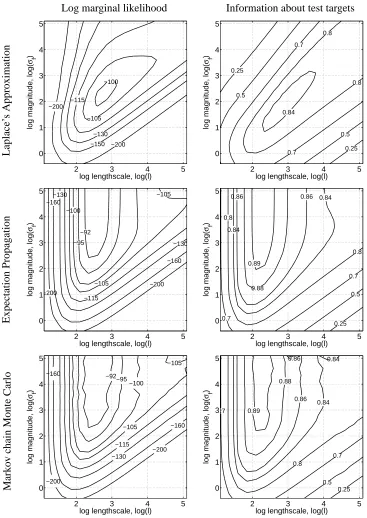
7.3 USPS Digits

We define a binary sub-problem from the USPS digit data3by considering 3’s vs. 5’s. We repeated the experiments described in the previous section for a slightly modified grid ofθ. Comparing the results shown in Figure 5 leads to similar results as mentioned above. The EP and MCMC results agree very well, given that the marginal likelihood comes as a 767 dimensional integral.

We now take a closer look at the approximations q(f_|

D

,θ) =

N

(f_|m,A)for a given value ofθ. We have chosen the values ln(σ) =3.35 and ln(`) =2.85 which are between the ML-II estimates of EP and Laplace’s method. Comparing the respective means of the approximations in Figure 6(a) we

2. Note that the agreement between the two seems to be limited by the accuracy of the AIS runs, as judged by the regularity of the contour lines; the tolerance is less than one unit on a (natural) log scale.

Log marginal likelihood Information about test targets L ap la ce ’s A p p ro x ima tio n −200 −150 −120 −120 −100 −100 −90 −80 −75 −70

log lengthscale, log(l)

log magnitude, log(

σ f

)

−1 0 1 2 3 4 5

−1 0 1 2 3 4 5 0 0 0.1 0.1 0.2 0.2 0.3 0.3 0.4 0.4 0.5 0.55

log lengthscale, log(l)

log magnitude, log(

σ f

)

−1 0 1 2 3 4 5

−1 0 1 2 3 4 5 E x p ec ta tio n P ro p ag atio n −120 −120 −100 −100 −90 −90 −80 −75 −75 −70 −65

log lengthscale, log(l)

log magnitude, log(

σ f

)

−1 0 1 2 3 4 5

−1 0 1 2 3 4 5 0

00.1 0.1

0.2 0.2 0.3 0.3 0.4 0.5 0.5 0.55 0.6

log lengthscale, log(l)

log magnitude, log(

σ f

)

−1 0 1 2 3 4 5

−1 0 1 2 3 4 5 M ar k o v ch ain M o n te C ar lo −120 −120 −100 −100 −90 −90 −80 −75 −75 −70 −65

log lengthscale, log(l)

log magnitude, log(

σ f

)

−1 0 1 2 3 4 5

−1 0 1 2 3 4 5 0 0 0.1 0.1 0.2 0.2 0.3 0.3 0.4 0.5 0.5 0.5 0.5 0.55 0.6

log lengthscale, log(l)

log magnitude, log(

σ f

)

−1 0 1 2 3 4 5

−1 0 1 2 3 4 5

Log marginal likelihood Information about test targets L ap la ce ’s A p p ro x ima tio n −200 −200 −150 −130 −115 −105 −100

log lengthscale, log(l)

log magnitude, log(

σ f

)

2 3 4 5

0 1 2 3 4 5 0.25 0.25 0.5 0.5 0.7 0.7 0.8 0.8 0.84

log lengthscale, log(l)

log magnitude, log(

σ f

)

2 3 4 5

0 1 2 3 4 5 E x p ec ta tio n P ro p ag atio n −200 −200 −160 −160 −130 −130 −115 −105 −105 −100 −95 −92

log lengthscale, log(l)

log magnitude, log(

σ f

)

2 3 4 5

0 1 2 3 4 5 0.25 0.5 0.7 0.7 0.8 0.8 0.84 0.84 0.86 0.86 0.88 0.89

log lengthscale, log(l)

log magnitude, log(

σ f

)

2 3 4 5

0 1 2 3 4 5 M ar k o v ch ain M o n te C ar lo

2 3 4 5

0 1 2 3 4 5

log lengthscale, log(l)

log magnitude, log(

σ f ) −92₋₉₅ −100 −105 −105 −115 −130 −160 −160 −200 −200 0.25 0.5 0.7 0.7 0.8 0.84 0.84 0.86 0.86 0.88 0.89

log lengthscale, log(l)

log magnitude, log(

σ f

)

2 3 4 5

0 1 2 3 4 5

−40 −20 0 20 40 −40

−30 −20 −10 0 10 20 30 40

m Laplace

m EP

Class 5 Class 3

−30 −20 −10 0

−20 −15 −10 −5 0

ln(w) Laplace

−ln(

σ

2 ) EP

Class 5 Class 3

(a) (b)

0 0.5 1

0 0.5 1

p* MCMC

p* Laplace & EP

Laplace p* EP p*

0 0.5 1

0 0.5 1

p* MCMC

p* Laplace & EP

Laplace p* EP p*

(c) (d)

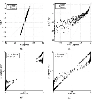
Figure 6: Comparison of approximations q(f_|

D

,θ) =

N

(f_|m,A)for a given value ofθ. Panel (a) shows a comparison of the means mi. In Panel (b) we compare the elements of the diago-nal matrices WiiandΣii. Panels (c) and (d) compare predictions p∗obtained by MCMC (abscissa) to predictions obtained from Laplace’s method and EP (ordinate). Panel (c) shows predictions on training cases and (d) shows predictions on test cases.

see that the magnitude of the means from the Laplace approximation is much smaller than from EP. The relation appears to be roughly linear. In Figure 6(b) we compare the elements of W andΣ−1

which cause the difference in the approximations (13) and (18) of the posterior covariance matrix A. We observe that the relatively large entries in W are larger than the corresponding entries inΣ−1_,

but in total W contains more small values thanΣ−1_{. The exact effect on the posterior covariance}

Figures 6(c-d) compare the predictive uncertainty p∗ resulting from the respective approxima-tions to MCMC predicapproxima-tions. For both training and test set we observe that EP and MCMC agree very well, while Laplace’s method shows over-conservative predictions.

−15 −10 −5 0 5

0 0.05 0.1 0.15 0.2

f MCMC samples Laplace p(f|D) EP p(f|D)

−400 −30 −20 −10 0 10

0.01 0.02 0.03 0.04 0.05 0.06 0.07

f MCMC samples Laplace p(f|D) EP p(f|D)

(a) (b)

Figure 7: Two marginal distributions p(f_i|

D

,θ)from the posterior. For Panel (a) we picked the

fi for which the posterior marginal is maximally skewed (see again Figure 1). The true posterior is approximated by a normalised histogram of 9000 samples of fiobtained by MCMC sampling. Panel (b) shows a case where EP and Laplace’s approximation differ significantly.

We now inspect the marginal distributions p(fi|

D

,θ)of single latent function values under the posterior approximation. We use hybrid MCMC to generate 9000 samples from the posterior of f for the aboveθ. For Laplace’s method and EP the approximated distribution is

N

(f_i|mi,Aii)where

m and A are found by the respective approximation techniques.

In general we observe that the marginal distributions of MCMC samples agree very well with the respective marginal distributions of the EP approximation. This supports the claim made in Section 5 where we argued that the marginal distributions of the posterior can be very similar to Gaussians, even if the posterior is a skew distribution. For Laplace’s approximation we find the mean to be underestimated and the marginal distributions to overlap with zero far more than the EP approximations. Figure 7(a) displays the marginal distribution and its approximations for which the MCMC samples show maximal skewness. Figure 7(b) shows a typical example where the EP approximation agrees very well with the MCMC samples. We show this particular example because under the EP approximation q(yi =1|

D

,θ)<0.1% but Laplace’s approximation gives

q(yi=1|

D

,θ)'18%.

7.4 Lower Bound Approximation

in-−250 −200

−150

−120 −120

−100 −100

−90 −90

−80 −80

−75 −75

−70

log lengthscale, log(l)

log magnitude, log(

σ f

)

Lower bound on log marginal likelihood

−1 0 1 2 3 4 5

−1 0 1 2 3 4 5

−200 −200

−160 −160

−130 −130

−115 −115

−105 −100

log lengthscale, log(l)

log magnitude, log(

σ f

)

Lower bound on log marginal likelihood

2 3 4 5

0 1 2 3 4 5

(a) Ionosphere (b) USPS 3’s vs. 5’s

Figure 8: Lower bound on marginal likelihood. Panel (a) shows the lower bound eq. (35) on the marginal likelihood for the Ionosphere data set (compare to left column of Figure 4). Panel (b) shows the value of the lower bound for the USPS 3’s vs. 5’s (compare to left column of Figure 5)

equality:

ln p(

D

_|θ) = ln

Z

p(y_|f)

N

(f_|0_{,K)df (35a)}

≥

Z

N

(f_|m,A)lnp(y|f)

N

(f|0,K)

N

(f_|m,A) df (35b)

=

m

∑

i=1 Z

N

(fi|mi,Aii)lnΦ(yifi)d fi

−1₂m>K−1m₋1

2tr(K

−1_{A) +}1

2ln|K

−1_A

|+m

2 . (35c)

Note that the one dimensional integrals in eq. (35c) have to be solved using numerical integration methods.

In sparse EP methods the Gaussian approximation is based on only a subset of observations and so the evidence (27) may be a bad approximation of the total evidence since it does not take all available data into account. Assume that the m points are only a subset of of a total of m0 observations. The lower bound (35c) can be extended to a lower bound on all m0 observations by including all points in the one dimensional integrals over the individual log likelihood terms.

respectively). However, the maxima of the lower bounds correspond to sub-optimal predictive per-formances compared to the maxima of the approximate marginal likelihood (27) (compare to the second row in Figures 4 and 5 respectively). Therefore for non-sparse EP approximations the use of (27) seems advisable, which is also computationally advantageous.

7.5 Benchmark Data Sets

In this section we compare the performance of Laplace’s method and Expectation Propagation for GPC on several well known benchmark problems for binary classification.

The Ionosphere, the Wisconsin Breast Cancer, and the Sonar data sets are taken from Hettich et al. (1998). The Leptograpsus Crabs and the Pima Indians Diabetes data sets were described by Ripley (1996). Note that for the Crabs data set we use the sex (not the colour) of the crabs as target variable. The largest data set in the comparison are the 3’s vs. 5’s from the USPS handwritten digits described above.

We standardise the inputs X to zero mean and unit variance. All data sets are randomly split into 10 folds of which one at a time is left out as a test set to measure the predictive performance of a model trained (or selected) on the remaining nine folds.

For GPC we implement model selection by ML-II hyper-parameter estimation. We use a con-jugate gradient optimisation routine to find a minimum

θML=argmin

θ −

ln q(

D

_|θ) (36)

of the negative log marginal likelihood approximated by Laplace’s method (15) and EP (27) respec-tively. For the respectiveθMLthe approximations

N

(f_|m,A)are computed and predictions are made for the left out test set. From the predictive distributions the average information (34) is computed and averaged over the ten folds. Furthermore the average error rate E is reported, which equals the average percentage of erroneous class assignments if prediction is understood as a decision problem with symmetric costs (thresholding the predictive uncertainty at 1/2).

In order to have a better absolute impression of the predictive performance we report the results of support vector machines (SVM) (Sch¨olkopf and Smola, 2002). We use the LIBSVM implemen-tation of C-SVM by Chang and Lin (2001) with a radial basis function kernel which is equivalent to the covariance function (33) up to the signal variance parameter. The values of the length scale parameter`and the regularisation parameter C are found by an inner loop of 5-fold cross-validation on the nine training folds respectively. We manually refine the parameter grids and repeat the cross-validation procedure until the performance stabilises.

We use the technique described by Platt (2000) to estimate predictive probabilities from an SVM. This is implemented by fitting a sigmoidal mapping from the unthresholded output of the SVM to the unit interval. The parameters of the mapping are estimated on the test set in the inner loop of 5-fold cross-validation.

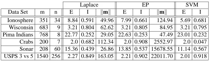
Results are summarised in Table 1. Comparing Laplace’s method to EP the latter shows to be more accurate both in terms of error rate and information. While the error rates are relatively similar the predictive distribution obtained by EP shows to be more informative about the test targets. As to be expected by now, the length of the mean vector _km_k shows much larger values for the EP approximations. Comparing EP and SVM the results are mixed.

Laplace EP SVM

Data Set m n E I _km_k E I _km_k E I

Ionosphere 351 34 8.84 0.591 49.96 7.99 0.661 124.94 5.69 0.681 Wisconsin 683 9 3.21 0.804 62.62 3.21 0.805 84.95 3.21 0.795 Pima Indians 768 8 22.77 0.252 29.05 22.63 0.253 47.49 23.01 0.232 Crabs 200 7 2.0 0.682 112.34 2.0 0.908 2552.97 2.0 0.047 Sonar 208 60 15.36 0.439 26.86 13.85 0.537 15678.55 11.14 0.567 USPS 3 vs 5 1540 256 2.27 0.849 163.05 2.21 0.902 22011.70 2.01 0.918

Table 1: Results for benchmark data sets. The first three columns give the name of the data set, number of observation m and dimension of inputs n. For Laplace’s method and EP the table reports the average error rate E, the average information I (34) and the average length km_kof the mean vector of the Gaussian approximation. For SVMs the error rate and the average information about the test targets are reported.

mean function (5a) at the test locations, which in turn depend on m only. Therefore the error rate is less sensitive to the accuracy of the approximation to the posterior, but of course depends on the ML-II estimated hyper-parameters, which differ between the methods. Also in the example shown in Figure 3(b) it can be observed that the latent mean functions differ but their sign matches very accurately.

For the Crabs data set all methods show the same error rate but the information content of the predictive distributions differs dramatically. For some test cases the SVM predicts the wrong class with large certainty. Because the mapping of the unthresholded output of the SVM to the predictive probability is estimated from a left out set, the mapping can be poor if too few errors are observed on this.

8. Conclusions

Our experiments reveal serious differences between Laplace’s method and EP when used in GPC models. The results corroborate the considerations about the two approximations based on the structure of the posterior given in Section 5. Although only a handful of data sets have been used in the study, we believe the conclusions to be well-founded and generally valid.

The EP approximation has shown to give results very close to MCMC both in terms of predictive distributions and marginal likelihood estimates. We have shown and explained why the marginal distributions of the posterior can be well approximated by Gaussians.

Further, the marginal likelihood values obtained by Laplace’s method and EP differ systemat-ically which will lead to different results of ML-II hyper-parameter estimation. The discrepancies are similar for different tasks. We were able to exemplify that the EP approximation of the marginal likelihood is accurate. To show this we described how AIS can be used to obtain unbiased estimates of the marginal likelihood for Gaussian process models.

In the experiments summarised in Table 1 we compared the predictive accuracy of GPC to sup-port vector machines. While the SVMs show a tendency to give lower error rates, the information contained in predictive distributions seems comparable. Conceptually GPC comes with the advan-tage that the Bayesian model selection can be used to set hyper-parameters by ML-II estimation, while the parameters of an SVM usually have to be set by cross-validation (gradient based methods exist, see e.g. Chapelle et al. (2002)).

In summary, we found that EP is the method of choice for approximate inference in binary GPC models, when the computational cost of MCMC is prohibitive. Very good agreement is achieved for both predictive probabilities and marginal likelihood estimates. In contrast, the Laplace approx-imation is so inaccurate that we advise against its use, especially when predictive probabilities are to be taken seriously.

Acknowledgments

Both authors acknowledge support by the German Research Foundation (DFG) through grant RA 1030/1. We would like to thank Tobias Pfingsten, Jeremy Hill and Matthias Seeger for comments and discussions.

Appendix A. Implementation of Laplace’s Approximation

In Sections 3 we described Laplace’s method for approximate inference in the GPC model and sketched the corresponding computations in Algorithm 1. In this appendix we describe our imple-mentation of the method in more detail. See also the appendices of Williams and Barber (1998).

Computing Laplace’s approximation

N

(f_|m,A) for given θ the main computational effort is involved in finding the maximum of the unnormalised log posterior ln

Q

(eq. (8)). Our implementa-tion uses Newton’s method to find the mode. In each Newton step the vector f is updated according to

ft+1 = ft₋(∇∇fln

Q

(ft))−1∇fln

Q

(ft) (37a) = (K−1_+W)−1_(Wft_+∇

fln

L

(ft)) (37b)

until convergence of f to the mode m. To ensure convergence the update is accepted if the value of the target function increases, otherwise the the step size is shortened until ln

Q

(ft+1_)>ln

_Q

_(ft_).

Computationally Newtons’s method is dominated by the repeated inversion of the Hessian. Since K can be poorly conditioned we use the identity

(K−1+W)−1=K₋KW12(I+W 1

2KW

1 2)−1W

1

such that only the well conditioned, positive definite matrix(I+W12KW 1

2)has to be inverted. In our implementation the inverse is computed from a Cholesky decomposition of this matrix. Note that W is a diagonal matrix with positive entries, so computing W12 is trivial.

Note that implementing the Newton updates (37) only requires the product of the inverse Hes-sian times the gradient which can be computed more efficiently using an iterative conjugate gradient method (Golub and Van Loan, 1989, ch. 10).

Having found the mode m the marginal likelihood approximation (15) and its derivatives can be computed. The approximate marginal likelihood takes the form

ln q(

D

_|θ) = ln

Q

(m) +m

2ln(2π) + 1

2ln|A| (39a)

= ln

L

(m)₋1

2m

>_K−1_m−1

2ln|I+KW|. (39b)

To avoid the direct inversion of K in the second term of (39b) we use the recurrence relation (37b). Let a=K−1m then by substituting (38) into (37b) we obtain:

a= (I₋W12(I+_W 1

2_KW

1 2)−1_W

1

2K)(Wm+∇_fln

L

(m)) ₍₄₀₎ such that m>K−1m=m>a. The determinant in eq. (39b) can be rewritten

ln_|I+KW_|=lnI+W 1

2_KW

1

2 ₍₄₁₎

and computed from the Cholesky decomposition, that was used to calculate the inverse in eq. (38). Note that if M=LL>is a Cholesky decomposition then ln_|M_|=2∑ln Lii.

During ML-II estimation (36) of hyper-parameters the approximate log marginal likelihood (39) is maximised as a function ofθ. Our implementation is based on a conjugate gradient optimisation routine such that we also need to compute the derivatives of (39b) with respect to the elements ofθ.

The dependency of the approximate marginal likelihood onθis two-fold:

∂ln q(

D

_|θ) ∂θi

=

∑

k,l

∂ln q(

D

_|θ) ∂Kkl

∂Kkl

∂θi

+∂ln q(

D

|θ) ∂m>

∂m ∂θi

(42)

there is a direct dependency via the terms involving K and an implicit dependency through the change in m (see also Williams and Barber (1998, Appendix B)).

The explicit derivative of eq. (39b) due to the direct dependency of the covariance matrix is

∑

k,l

∂ln q(

D

_|θ) ∂Kkl

∂Kkl

∂θi

= 1

2m

>_K−1∂K ∂θi

K−1m₋1

2tr

(I+KW)−1∂K ∂θi

W

(43)

where the first term is computed using a (40) and the inverse in the second term can be rewritten as

(I+KW)−1=I₋(K−1+W)−1W (44)

where the inverse (38) is already known.

The implicit derivative accounts for the dependency of eq. (39b) onθdue to change in the mode

m. Differentiating eq. (39a) with respect to m reduces to∂ln_|A_|/∂m since m is the maximum of ln

Q

and therefore∂ln

Q

/∂m vanishes.

∂ln q(

D

_|θ) ∂m>

∂m ∂θi

= ₋1

2

∂|K−1_+W| ∂m>

∂m ∂θi

= ₋1

2(K

−1_+W)−1 ∂W ∂m>

∂m ∂θi

The dependency of m onθiis obtained by differentiating (11a) at m:

0=∇fln

L

(m)−K−1m =⇒ m=K∇fln

L

(m) (46)

so

∂m ∂θi

= ∂K

∂θi

∇fln

L

(m) +K∇∇fln

L

(m) ∂m ∂θi

= (I+KW)−1∂K

∂θi

∇fln

L

(m) (47)

and we have both terms necessary to compute the gradient (42).

To compute the predictive probability p_∗=p(y_∗=1_|x_∗)for a test input x_∗the predictive distri-bution (5) of the latent function value is

N

(f_∗|µ_∗,σ2

∗)where

µ_∗ = k>_∗K−1m=k>_∗a (48a)

σ2

∗ = k(x∗,x∗)−k>∗W 1 2(I+W

1

2KW

1 2)−1W

1 2k

∗ (48b)

and p_∗can be computed from eq. (6).

Due to the Cholesky decomposition in (38) computing Laplace’s approximation is

O

(m3). How-ever, following the implementation we described in this section a Cholesky decomposition has to be computed once per Newton step and all other quantities can be computed from it in at most

O

(m2). The number of Newton steps necessary depends on the convergence criterion, the initialisation of f and the hyper-parametersθ.

Appendix B. Implementation of Expectation Propagation

In this appendix we describe details of our implementation of EP as described in Section 4 and summarised in Algorithm 2. See also the appendices of Seeger (2003).

In our implementation the site functions (17) are parameterised in terms of natural parameters

σ−2

i andσ−i 2µi. For givenθthe algorithm starts by initialising A=K andσ−i 2=0 andσ−i 2µi=0. The algorithm proceeds by updating the site parameters in random order. In each sweep every site function is updated following equations (23), (25), and (26). After each update of a site function the effect on m and A has to be computed according to (18). The change in A can be computed using a rank one update. Letδbe the change inσ−_i 2due to the update and eithe vector whose ith entry is 1 and all other 0. The relation

(K−1+Σ−1₊δe_ie>

i )−1=A−Aei(Aii+δ−1)−1e>i A (49)

can be used to update A. Each single update is

O

(m2)and repeated m times per sweep, such that the EP algorithm is

O

(m3)in time. Because of accumulating numerical errors, after a complete sweep over all site functions we recompute the matrix A from scratch. For numerical stability we rewrite

A= (K−1+Σ−1₎−1_=K−KΣ−12(I+Σ−21_KΣ−21)−1Σ−12_{K (50)} and compute the inverse from the Cholesky decomposition of(I+Σ−12KΣ−12).

After convergence the approximate log marginal likelihood (27) can be computed and its partial derivatives with respect to the hyper-parameters:

∂ln q(

D

_|θ) ∂θi

=₋1

2tr

∂K

∂θi

(K+Σ₎−1_−(K+Σ₎−1_µµ>_(K+Σ₎−1

which do not depend on the Zi(Seeger, 2005).

The inverse of K+Σ_{can be computed from the inverse in eq. (50):}

(K+Σ₎−1₌Σ−12(I+Σ−21_KΣ−12)−1Σ−12 . ₍₅₂₎

For computing the log marginal likelihood (27) also the determinant|K+Σ_{|has to be computed.}

By rewriting

ln_|K+Σ_|=ln(|Σ_||I+Σ−1_{K|) =ln|}Σ_|+ln|I+Σ−12KΣ− 1

2| (53)

we obtain an expression in which the first term is a determinant of a diagonal matrix and the second term can be computed from the Cholesky decomposition that was used to compute the inverse in eq. (50).

To compute the predictive probability p_∗=p(y_∗=1_|x_∗)for a test input x_∗the predictive distri-bution (5) of the latent function value is

N

(f_∗|µ_∗,σ2

∗)where

µ_∗ = k>_∗(K+Σ₎−1_{µ (54a)}

σ2

∗ = k(x∗,x∗)−k>∗(K+Σ)−1k∗ (54b)

and p_∗can be computed from eq. (6).

The EP algorithm is of computational complexity

O

(m3) due to the computations for updat-ing A. However, per sweep the computation of A (50) and the m rank one updates sum to more computational effort compared to Laplace’s method.

References

P. Abrahamsen. A review of Gaussian random fields and correlation functions. Technical Report 917, Norwegian Computing Center, Oslo, 1997.

C.-C. Chang and C.-J. Lin. LIBSVM: A library for Support Vector Machines, 2001.

http://www.csie.ntu.edu.tw/_∼cjlin/libsvm.

O. Chapelle, V. Vapnik, O. Bousquet, and S. Mukherjee. Choosing multiple parameters for support vector machines. Machine Learning, 46(1):131–159, 2002.

W. Chu and Z. Ghahramani. Gaussian processes for ordinal regression. Journal of Machine

Learn-ing Research, 6:1019–1041, 2005.

L. Csat´o and M. Opper. Sparse online Gaussian processes. Neural Computation, 14(2):641–669, 2002.

S. Duane, A. D. Kennedy, B. J. Pendleton, and D. Roweth. Hybrid Monte Carlo. Physics Letters B, 195(2):216–222, 1987.

A. Gelman and X.-L. Meng. Simulating normalizing constants: From importance sampling to bridge sampling to path sampling. Statistical Science, 13(2):163–185, 1998.

M. N. Gibbs and D. J. C. MacKay. Variational Gaussian process classifiers. IEEE Transactions on

Neural Networks, 11(6):1458–1464, 2000.

G. H. Golub and C. F. Van Loan. Matrix Computations. John Hopkins University Press, Baltimore, second edition, 1989.

S. Hettich, C. L. Blake, and C. J. Merz. UCI repository of machine learning databases, 1998.

http://www.ics.uci.edu/_∼mlearn/MLRepository.html.

R. E. Kass and A. E. Raftery. Bayes factors. Journal of the American Statistical Association, 90 (430):773–795, 1995.

N. Lawrence, M. Seeger, and R. Herbrich. Fast sparse Gaussian process methods: The informa-tive vector machine. In S. Becker, S. Thrun, and K. Obermayer, editors, Advances in Neural

Information Processing Systems 15, pages 609–616, Cambridge, MA, 2003. The MIT Press.

J. S. Liu. Monte Carlo Strategies in Scientific Computing. Springer, New York, 2001.

D. J. C. MacKay. Comparison of approximate methods for handling hyperparameters. Neural

Computation, 11(5):1035–1068, 1999.

D. J. C. MacKay. Information Theory, Inference and Learning Algorithms. Cambridge University Press, Cambridge, UK, 2003.

T. P. Minka. A Family of Algorithms for Approximate Bayesian Inference. PhD thesis, Department of Electrical Engineering and Computer Science, MIT, 2001.

R. M. Neal. Regression and classification using Gaussian process priors. In J. M. Bernardo, J. O. Berger, A. P. Dawid, and A. F. M. Smith, editors, Bayesian Statistics 6, pages 475–501. Oxford University Press, 1998.

R. M. Neal. Annealed importance sampling. Statistics and Computing, 11:125–139, 2001.

A. O’Hagan. Curve fitting and optimal design for prediction. Journal of the Royal Statistical Society,

Series B, 40(1):1–42, 1978.

M. Opper and O. Winther. Gaussian processes for classification: Mean-field algorithms. Neural

Computation, 12(11):2655–2684, 2000.

J. C. Platt. Probabilities for SV machines. In A. J. Smola, P. L. Bartlett, B. Sch¨olkopf, and D. Schu-urmans, editors, Advances in Large Margin Classifiers, pages 61–73. The MIT Press, Cambridge, MA, 2000.

C. E. Rasmussen and C. K. I Williams. Gaussian Processes for Machine Learning. The MIT Press, Cambridge, MA, 2006. In press.

B. D. Ripley. Pattern Recognition and Neural Newtorks. Cambridge University Press, Cambridge, UK, 1996.

B. Sch¨olkopf and A. J. Smola. Learning with Kernels. The MIT Press, Cambridge, MA, 2002.

M. Seeger. PAC-Bayesian generalisation error bounds for Gaussian process classification. Journal

of Machine Learning Research, 3:233–269, 2002.

M. Seeger. Bayesian Gaussian Process Models: PAC-Bayesian Generalisation Error Bounds and

Sparse Approximations. PhD thesis, University of Edinburgh, 2003.

M. Seeger. Expectation propagation for exponential families, 2005. Note obtainable from

http://www.kyb.tuebingen.mpg.de/_∼seeger.

C. K. I. Williams and D. Barber. Bayesian classification with Gaussian processes. IEEE