Multi-task Sparse Structure Learning
with Gaussian Copula Models
Andr´e R. Gon¸calves [email protected]
Fernando J. Von Zuben [email protected]
School of Electrical and Computer Engineering University of Campinas
S˜ao Paulo, Brazil
Arindam Banerjee [email protected]
Computer Science Department
University of Minnesota - Twin Cities Minneapolis, USA
Editor:Urun Dogan, Marius Kloft, Francesco Orabona, and Tatiana Tommasi
Abstract
Multi-task learning (MTL) aims to improve generalization performance by learning multi-ple related tasks simultaneously. While sometimes the underlying task relationship struc-ture is known, often the strucstruc-ture needs to be estimated from data at hand. In this paper, we present a novel family of models for MTL, applicable to regression and classification problems, capable of learning the structure of tasks relationship. In particular, we consider a joint estimation problem of the tasks relationship structure and the individual task pa-rameters, which is solved using alternating minimization. The task relationship revealed by structure learning is founded on recent advances in Gaussian graphical models endowed with sparse estimators of the precision (inverse covariance) matrix. An extension to include flexible Gaussian copula models that relaxes the Gaussian marginal assumption is also pro-posed. We illustrate the effectiveness of the proposed model on a variety of synthetic and benchmark data sets for regression and classification. We also consider the problem of com-bining Earth System Model (ESM) outputs for better projections of future climate, with focus on projections of temperature by combining ESMs in South and North America, and show that the proposed model outperforms several existing methods for the problem.
Keywords: multi-task learning, structure learning, Gaussian copula, probabilistic graph-ical model, sparse modeling
1. Introduction
Kim and Xing, 2010; Kumar and Daume III, 2012; Yang et al., 2013). Meanwhile MTL has been applied to problems ranging from object detection in computer vision, going through web image and video search (Wang et al., 2009), and achieving multiple microarray data set integration in computational biology (Widmer and R¨atsch, 2012).
Much of the existing work in MTL assumes the existence of a priori knowledge about the task relationship structure (see Section 2). However, in many problems there is only a high level understanding of those relationships, and hence the structure of the task relationship needs to be estimated from the data. Recently, there have been attempts to explicitly model the relationship and incorporate it into the learning process (Zhang and Yeung, 2010; Zhang and Schneider, 2010; Yang et al., 2013). In the majority of these methods, the tasks dependencies are represented as unknown hyper-parameters in hierarchical Bayesian models and are estimated from the data. As will be discussed in Section 2, many of these methods are either computationally expensive or restrictive on dependence structure complexity.
Instructure learning, we estimate the (conditional) dependence structures between ran-dom variables in a high-dimensional distribution, and major advances have been achieved in the past few years (Banerjee et al., 2008; Friedman et al., 2008; Cai et al., 2011; Wang et al., 2013). In particular, assuming sparsity in the conditional dependence structure, i.e., each variable is dependent only on a few others, there are estimators based on convex (sparse) optimization which are guaranteed to recover the correct dependence structure with high probability, even when the number of samples is small compared to the number of variables.
In this paper, we present a family of models for MTL, for regression and classification problems, which are capable of learning the structure of task relationships and parameters for individual tasks. The problem is posed as a joint estimation where parameters of the tasks and relationship structure are learned using alternating minimization. This paper is an extension of our early work (Gon¸calves et al., 2014), as it further includes improvements on the task relationship modeling and can now handle a wider spectrum of problems.
The relationship structure is modeled by either imposing a prior over the features across tasks (Section 3.3) or assuming correlated residuals (Section 3.7). We can use of a vari-ety of methods from the structure learning literature to estimate the relationships. The formulation can be extended to Gaussian copula models (Liu et al., 2009; Xue and Zou, 2012), which are more flexible as it does not rely on strict Gaussian assumptions and has shown to be more robust to outliers. The resulting estimation problems are solved using suitable first order methods, including proximal updates (Beck and Teboulle, 2009) and alternating direction method of multipliers (Boyd et al., 2011). Based on our modeling, we show that MTL can benefit from advances in the structure learning area. Moreover, any future development in the area can be readily used in the context of MTL.
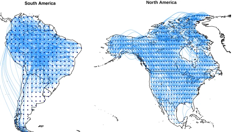
In addition to evaluation on synthetic and benchmark data sets, we consider the problem of predicting air surface temperature in South and North America. The goal here is to combine outputs from Earth System Models (ESMs) reported by various countries to the Intergovernmental Panel on Climate Change (IPCC), where the regression problem at each geographical location forms a task. The weight on each model at each location forms the “skill” of that model, and the hope is that outputs from skillful models in each region can be more reliable for future projections of temperature. MSSL is able to identify geographically nearby regions as related tasks, which is meaningful for temperature prediction, without any previous knowledge of the spatial location of the tasks, and outperforms baseline approaches. The remainder of the paper is structured as follows. Section 2 briefly discusses the related work in multi-task learning. Section 3 presents an overview and gentle introduction to the proposed multi-task sparse structure learning (MSSL) approach. Section 3.3 discusses a specific form of MSSL where the task structure dependence is learned based on the task coefficients. The MSSL is extended to the Gaussian copula MSSL in Section 3.6. Section 3.7 discusses another specific form of MSSL where the task structure dependence is learned based on the task residuals. Section 4 presents experimental results on regression and classification using synthetic, benchmark, and climate data sets. We conclude in Section 5.
Notation. We denote bymthe number of tasks,dthe problem dimension, supposed to be the same for all learning tasks, andnk the number of samples for thek-th task. Xk∈Rnk×d and yk ∈ Rnk×1 are the input and output data for the k-th task. Let W ∈ Rd×m be the parameter matrix, where columns are vector parameters wk ∈ Rd, k = 1, ..., m, for the tasks. (x)+= max(0, x). LetS+p be the set of p×ppositive semidefinite matrices. For any matrixA, tr(A) is the trace operator,kAk1andkAkF are the`1-norm and Frobenius norm ofA, respectively. A◦B denotes the Hadamard (element-wise) product of the matricesA
and B. Ip is the p×p identity matrix and 0p×p is a matrix full of zeros. For anm-variate
random variableV = (V1, ..., Vm), we denote byV\{i,j} the set of marginals exceptiand j.
2. Related Work
MTL has attracted a great deal of attention in the past few years and consequently many algorithms have been proposed (Evgeniou and Pontil, 2004; Argyriou et al., 2007; Xue et al., 2007; Jacob et al., 2008; Obozinski et al., 2010; Zhou et al., 2011b; Zhang and Yeung, 2010; Yang et al., 2013; Gon¸calves et al., 2014). We will present a general view of the methods and discuss in more details those that are more related to ours.
The majority of the proposed methods fall into the class of regularized multi-task learn-ing, which has the form
min W
m X
k=1
nk
X
i=1
` f(xik,wk), yki
!
+R(W),
where `(·) is the loss function such as squared, logistic, and hinge loss; R(W) is a reg-ularization function for W that can be designed to enforce some sharing of information between tasks. In such a context, the goal of MTL is to estimate the tasks parameters
W= [w1, ...,wm], while taking into account the underlying relationship among tasks.
tasks. Some methods assume a fixed structure a priori, while others try to estimate it from the data. In the following we present a representative set of methods from these categories.
2.1 MTL with All Tasks Related
One class of MTL methods assumes that all tasks are related and the information about tasks are selectively shared among all tasks, with the hypothesized structure of the param-eter matrixW controlling how the information is shared.
Evgeniou and Pontil (2004) considered the scenario that all tasks are related in a way that the model parameters are close to some mean model. Motivated by the sparsity inducing property of the `1-norm (Tibshirani, 1996), the idea of structured sparsity has been widely explored in MTL algorithms. Argyriou et al. (2007) assumed that there exists a subset of features that is shared for all the tasks and imposed an`2,1−norm penalization on the matrix W to select such set of features. In the dirty-model proposed in Jalali et al. (2010) the matrix W is modeled as the sum of a group sparse and an element-wise sparse matrix. The sparsity pattern is imposed by `q and `1-norm regularizations. Similar
decomposition was assumed in Chen et al. (2010), but thereWis a sum of an element-wise sparse (`1) and a low-rank (nuclear norm) matrix. The assumption that a low-dimensional subspace is shared by all tasks is explored in Ando et al. (2005), Chen et al. (2009), and Obozinski et al. (2010). For example, in Obozinski et al. (2010) a trace norm regularization on W was used to select the common low-dimensional subspace.
2.2 MTL with Cluster Assumption
Another class of MTL methods assumes that not all tasks are related, but instead the relatedness is in a group (cluster) structure, that is, mutually related tasks are in the same cluster, while unrelated tasks belong to different clusters. Information is shared only by those tasks belonging to the same cluster. The problem then involves estimating the number of clusters and the matrix encoding the assignment cluster information.
In Bakker and Heskes (2003) task clustering was enforced by considering a mixture of Gaussians as a prior over task parameters. Evgeniou et al. (2005) proposed a task clustering regularization to encode cluster information in the MTL formulation. Xue et al. (2007) employed a Dirichlet process prior over the task coefficients to encourage task clustering and the number of clusters was someway automatically determined by the prior.
2.3 MTL with Dependence Structure Learning
Recently, there have been some proposals to estimate and incorporate the dependence among the tasks into the learning process. These methods are the most related to ours.
in the task parameter learning step, therefore, the inverse of the covariance matrix needed to be computed at every iteration. We, on the other hand, do not constrain the complexity of our model and also learn the inverse of the covariance matrix directly, which tends to be more stable than computing covariance and then inverting it.
Zhang and Schneider (2010) also used a matrix-variate normal prior over W. The two matrix hyper-parameters explicitly represent the covariance among the features (assuming the same feature relationships in all tasks) and covariance among the tasks, respectively. Sparse inducing penalization on the inverse covariance Ω of both is added into the for-mulation. Unlike Zhang and Yeung (2010), both matrices are learned in an alternating minimization algorithm and can be computationally prohibitive in high dimensional prob-lems due to the cost of modeling and estimating the feature covariance.
Yang et al. (2013) also assumed a matrix normal prior for W. However, the row and column covariance hyperparameters have a Matrix Generalized Inverse Gaussian (MGIG) prior distribution. The mean of matrixWis factorized as the product of two matrices that also has matrix-variate normal distribution as a prior. The model inference is done via a variational Expectation Maximization (EM) algorithm. Due to the lack of a closed form expression to compute statistics of the MGIG distribution, the method resort to the use of sampling techniques, which can be slow for high-dimensional problems.
Rothman et al. (2010) also enforced sparsity on bothW andΩ. Similar to our residual-based MSSL formulation, it differs in two aspects: (i) our formulation allows a richer class of conditional distributionp(y|x), namely distributions in the exponential family, rather than simply Gaussian; and (ii) we employ a semiparametric Gaussian copula model to capture task relationship, which does not rely of Gaussian assumption on the marginals and have shown to be more robust to outliers (Liu et al., 2012), then traditional Gaussian model used in Rothman et al. (2010). As will be seen in the experiments, the MSSL method with copula models produced more accurate predictions. Rai et al. (2012) extended the formulation in Rothman et al. (2010) to model feature dependence, additionally to the task dependence modeling. However, it is computationally prohibitive for high-dimensional problems, due to the cost of estimating another precision matrix for feature dependence.
Zhou and Tao (2014) used copula as a richer class of conditional marginal distributions
p(yk|x). As copula models express the joint distribution p(y|x) from the set of marginal
distributions, this formulation allows marginals to have arbitrary continuous distributions. Output correlation is exploited via the sparse inverse covariance in the copula function, which is estimated by a procedure based on proximal algorithms. Our method also covers a rich class of conditional distributions, the exponential family that includes Gaussian, Bernoulli, Multinomial, Poisson, and Dirichlet, among others. We use Gaussian copula models to capture tasks dependence, instead of explicitly modeling marginal distributions.
3. Multi-task Sparse Structure Learning
3.1 Structure Estimation in Gaussian Graphical Models
Here we describe the undirected graphical model used to capture the underlying linear dependence structure of our multi-task learning framework.
LetV = (V1, . . . , Vm) be anm-variate random vector with joint distributionp(V). Such
distribution can be characterized by an undirected graphG = (V,E), where the vertex set
V represents them covariates of V and edge set E represents the conditional dependence relations between the covariates of V. If Vi is conditionally independent of Vj given the
other variables, then the edge (i, j) is not in E. AssumingV ∼ N(0,Σ), the missing edges correspond to zeros in the inverse covariance matrix orprecision matrix given byΣ−1 =Ω, i.e., (Σ−1)ij = 0 ∀(i, j)∈/ E (Lauritzen, 1996).
Classical estimation approaches (Dempster, 1972) work well when m is small. Given, that we have n i.i.d. samples v1, . . . , vn from the distribution, the empirical covariance
matrix is Σˆ = n1 Pn
i=1(vi−v¯)
>(v
i −v¯), where ¯v = 1nPni=1vi. However, when m > n, ˆ
Σ is rank-deficient and its inverse cannot be used to estimate the precision matrix Ω. Nonetheless, for a sparse graph, i.e. most of the entries in the precision matrix are zero, several methods exist to estimateΩ(Friedman et al., 2008; Boyd et al., 2011).
3.2 MSSL Formulation
For ease of exposition, let us consider a simple linear model for each task: yk =Xkwk+ξk
where wk is the parameter vector for task k and ξk denotes the residual error. The
pro-posed MSSL method estimates both the task parameterswk for all tasks and the structure dependence, based on some information from each task. Further, the dependence structure is used as inductive bias in thewklearning process, aiming at improving the generalization
capability of the tasks.
We investigate and formalize two ways of learning the relationship structure (a graph indicating the relationship among the tasks), represented by Ω: (a) modeling Ω from the task specific parameters wk,∀k = 1, ..., m and (b) modeling Ω from the residual errors
ξk,∀k= 1, ..., m. Based on how we model Ω, we propose p-MSSL (from tasks parameters) and r-MSSL (from residual error). Both models are discussed in the following sections.
At a high level, the estimation problem in such MSSL approaches takes the form:
min
W,Ω0 L((Y,X),W) +B(W,Ω) +R1(W) +R2(Ω), (1) whereL(·) denotes suitable task specific loss function,B(·) is the inductive bias term, and
R1(·) andR2(·) are suitable sparsity inducing regularization terms. The interaction between parameterswk and the relationship matrixΩis captured by the B(·) term. Notably, when Ωk,k0 = 0, the parameters wk and wk0 have no influence on each other. Sections 3.3 to 3.7
delineate the modeling details behind MSSL algorithms and how it leads to the solution of the optimization problem in (1).
3.3 Parameter Precision Structure
scenario, we propose to use the precision matrix Ω ∈ Rm×m in order to capture pairwise
partial correlations between tasks.
In the parameter precision structure based MSSL (p-MSSL) model we assume that features across tasks (rows wjˆ of the matrixW) follows a multivariate Gaussian distribution with zero mean and covariance matrix Σ, i.e., ˆwj ∼ N(0,Σ) ∀j= 1, ..., d, where Σ−1=Ω.
The problem of interest is to estimate both the parameters w1, . . . ,wm and the precision
matrix Ω. By imposing such a prior over the rows of W, we are capable of explicitly estimating the dependency structure among the tasks via the precision matrix Ω.
With a multivariate Gaussian prior over the rowsof W, its posterior can be written as
p(W|(X,Y),Ω)∝ m Y k=1 nk Y i=1
p yikxik,w>k
d Y
j=1
p( ˆwj|Ω), (2)
where the first term in the right hand side denotes the conditional distribution of the response given the input and parameters, and the second term denotes the prior overrows
of W. In this paper, we consider the penalized maximization of (2), assuming that the parameter matrix W and the precision matrix Ω are sparse, i.e., contain few non-zero elements. In the following, we provide two specific instantiations of this model. First, we consider a Gaussian conditional distribution, wherein we obtain the well known least squares regression problem (Section 3.3.1). Second, for discrete labeled data, choosing a Bernoulli conditional distribution leads to a logistic regression problem (Section 3.3.2).
3.3.1 Least Squares Regression
Assume that
p ykixik,wk
=N1
yik
w
>
kxik, σ2k
,
where it is considered for ease of exposition that the variance of the residualsσ2k= 1,∀k= 1, ..., m, though it can be incorporated in the model and learned from the data. We can write this optimization problem as minimization of the negative logarithm of (2), which corresponds to a regularized linear regression problem
min
W,Ω0
1 2 m X k=1 nk X i=1
w>kxik−yki2
−d
2log|Ω|+ 1
2tr(WΩW
>).
Further, assuming that Ω and W are sparse, we add `1-norm regularizers over both parameters. In the case one task has a much larger number of samples compared to the others, it may dominate the empirical loss term. To avoid such bias we modify the cost function and compute the weighted average of the empirical losses of the form
min W,Ω0
m X k=1 1 nk nk X i=1
w>kxik−yik 2
−dlog|Ω|+λ0tr(WΩW>) +λ1kWk1+λ2kΩk1, (3)
independence, that is, Ωij = 0 if and only ifwi⊥⊥wj|W\{i,j}. Then, enforcing sparsity on
Ωwill highlight the conditional independence among tasks parameters.
In this formulation, the term involving the trace of the outer product tr(WΩW>) affects therows of W, such that if Ωij 6= 0, thenwi andwj are constrained to be similar.
Although the problem is not jointly convex on W andΩ, it is in fact biconvex, that is, fixingΩthe problem is convex onW, and vice-versa. So, the associated biconvex function in problem (3) is split into two convex functions exhibited in (4a) and (4b). Then, one can use an alternating optimization procedure that updates W and Ω by fixing one of them and solving the corresponding convex optimization problem (Gorski et al., 2007), given by
fΩ(W;X,Y, λ0, λ1) =
m X
k=1 1
nk nk
X
i=1
(w>kxik−yki)2+λ0tr(WΩW>) +λ1kWk1, (4a)
fW(Ω;X,Y, λ0, λ2) =λ0tr(WΩW>)−dlog|Ω|+λ2kΩk1. (4b) The alternating minimization algorithm proceeds as described in Algorithm 1. The procedure is guaranteed to converge to a partial optimum Gorski et al. (2007), since the original problem (3) is biconvex and convex in each argument ΩandW.
Algorithm 1:Multitask Sparse Structure Learning (MSSL) algorithm
Data: {Xk,yk}mk=1. // training data for all tasks
Input: λ0, λ1, λ2 >0. // penalty parameters chosen by cross-validation
Result: W,Ω. // estimated parameters
begin
/* Ω0 is initialized with identity matrix and */
/* W0 with random numbers in [-0.5,0.5]. */
InitializeΩ0 and W0 t= 1
repeat
W(t+1)= argmin
W fΩ(t)(W) // optimize W with Ω fixed
Ω(t+1)= argmin
Ω fW(t+1)(Ω) // optimize Ω with W fixed
t=t+ 1
untilstopping condition met end
Update for W: The update step involving (4a) is an `1−regularized quadratic problem. Thus the problem is an`1-penalized quadratic optimization program, which we solve using established proximal gradient descent methods such as FISTA (Beck and Teboulle, 2009). TheW-step can be seen as a general case of the formulation in Subbian and Banerjee (2013) in the context of climate model combination, where in our proposalΩis any positive definite precision matrix, rather than a fixed Laplacian matrix as in Subbian and Banerjee (2013). In the class of proximal gradient methods the cost function h(x) is decomposed as
typically non-smooth. The accelerated proximal gradient iterates as follows
zt+1 :=wtk+ωt wtk−wtk−1 wkt+1 :=proxρtg zt+1−ρt∇f zt+1
, (5)
whereωt∈[0,1) is an extrapolation parameter andρt is the step size. Theωtparameter is chosen as ωt= (ηt−1)/ηt+1, with ηt+1 = (1 +
p
1 + 4η2
t)/2 as done in Beck and Teboulle
(2009) and ρt can be computed by a line search. The proximal operator associated with the`1-norm is the soft-thresholding operator
proxρt(x)i = (|xi| −ρt)+sign(xi) (6) The convergence rate of the algorithm is O(1/t2) (Beck and Teboulle, 2009). Considering the squared loss, the gradient for the weights of thek-th task is computed as
∇f(wk) =
1
nk
(X>kXkwk−X>kyk) +λ0ψk, (7)
where ψk is thek-th column of matrix Ψ= 2WΩ= ∂W∂ tr(WΩW>). Note that the first two terms of the gradient, which come from the loss function, are independent for each task and then can be computed in parallel.
Update for Ω: The update step for Ω involving (4b) is known as the sparse inverse covariance selection problem and efficient methods have been proposed recently (Banerjee et al., 2008; Friedman et al., 2008; Boyd et al., 2011; Cai et al., 2011; Wang et al., 2013). Re-writing (4b) in terms of the sample covariance matrixS, the minimization problem is
min
Ω0 λ0tr(SΩ)−log|Ω|+
λ2
d kΩk1, (8)
where S = 1dW>W. This formulation will be useful to connect to the Gaussian copula extension in the next section. As λ2 is a user defined parameter, the factor 1d can be incorporated intoλ2.
To solve the minimization problem (8) we use an efficient Alternating Direction Method of Multiplies (ADMM) algorithm (Boyd et al., 2011). ADMM is a strategy that is intended to blend the benefits of dual decomposition and augmented Lagrangian methods for con-strained optimization. It takes the form of adecomposition-coordinationprocedure, in which the solutions to small local problems are coordinated to find a solution to a large global problem. We refer interested readers to Boyd et al. (2011) in its Section 6.5 for details on the derivation of the updates.
In ADMM, we start by forming the augmented Lagrangian function of the problem (8)
Lρ(Θ,Z,U) =λ0tr(SΘ)−log|Θ|+λ2kZk1+
ρ
2kΘ−Z+Uk 2
F − ρ
2kUk 2
F, (9)
Given the matrix S(t+1) = 1d(W(t+1))>W(t+1) and setting Θ0 = Ω(t), Z0 = 0m×m, and U0 =0m×m, the ADMM for the problem (8) consists of the iterations:
Θl+1= argmin
Θ0 λ0tr(S
l+1Θ)−log|Θ|+ρ
2kΘ−Z
l+Ulk2
F (10a)
Zl+1= argmin
Z λ2kZk1+
ρ
2kΘ
l+1−Z+Ulk2
F (10b)
Ul+1=Ul+Θl+1−Zl+1. (10c)
The output of the ADMM is Ωt+1=ΘL, whereL is the number of steps for convergence. Each ADMM step can be solved efficiently. For the Θ-update, we can observe, from the first order optimality condition of (10a) and the implicit constraint Θ 0, that the solution consists basically of a singular value decomposion.
The Z-update (10b) can be computed in closed form, as follows
Zl+1 =Sλ2/ρ
Θl+1+Ul
, (11)
where Sλ2/ρ(·) is an element-wise soft-thresholding operator (Boyd et al., 2011). Finally,
the updates for U in (10c) are already in closed form.
3.3.2 Log Linear Models
As described previously, our model can also be applied to classification. Let us assume that
p ykixik,wk
= Be
yki
h
w>kxik
,
whereh(·) is the sigmoid function, and Be(p) is a Bernoulli distribution. Therefore, following the same construction as in Section 3.3.1, parametersWand Ωcan be obtained by solving the following minimization problem:
min W,Ω0
m X
k=1
1
nk nk X
i=1
yikw
>
kx i
k−log(1 +e
wk>xik
)+λ0tr(WΩW
>
)−dlog|Ω|+λ1kWk1+λ2kΩk1. (12)
The loss function is the logistic loss, where we have considered a 2-class classification set-ting. In general, we can consider any generalized linear model (GLM) (Nelder and Baker, 1972), with different link functions h(·), and therefore different probability densities, such as Poisson, Multinomial, and Gamma, for the conditional distribution. For any such model, our framework requires the optimization of an objective function of the form
min W,Ω0
m X
k=1
L(yk,Xkwk) +λ0tr(WΩW>)−dlog|Ω|+λ1kWk1+λ2kΩk1, (13)
whereL(·) is a convex loss function obtained from a GLM.
3.4 p-MSSL Interpretation as Using a Product of Distributions as Prior
From a probabilistic perspective, sparsity can be enforced using the so-called sparsity pro-moting priors, such as the Laplacian-like (double exponential) prior (Park and Casella, 2008). Accordingly, instead of exclusively assuming a multivariate Gaussian distribution as a prior for the rows of tasks parameter matrixW, we can consider an improper prior which consists of the product of multivariate Gaussian and Laplacian distributions, of the form
pGL
ˆ
wj|µ,Ω, λ0, λ1
∝ |Ω|1/2exp
−λ0
2 ( ˆwj−µ)
>Ω( ˆw
j−µ)
exp
−λ1
2 kwˆjk1
, (14)
where we introduced the λ0 parameter to control the strength of the Gaussian prior. By changingλ0 andλ1, we alter the relative effect of the two component priors in the product. Setting λ0 to one and λ1 to zero, we return to the exclusive Gaussian prior as in (2). Hence,p-MSSL formulation in (3) can be seen exactly (assuming sparse precision matrix in Gaussian prior) as a MAP inference of the conditional posterior distribution (withµ= 0)
p
W|(X,Y),Ω ∝ K Y k=1 Nk Y i=1
Nyik|wk>xik, σ2
YD
j=1
pGL
ˆ
wj|Ω, λ0, λ1
. (15)
Equivalently, the p-MSSL with GLM formulation as in (13) can be obtained by replacing the conditional Gaussian in (15) by another distribution in the exponential family.
3.5 Adding New Tasks
Suppose now that, after estimating all the tasks parameters and the precision matrix, a new task arrives and needs to be trained. This is known as the asymmetric MTL problem (Xue et al., 2007). Clearly, it will be computationally prohibitive in real applications to re-run the MSSL every time a new task arrives. Fortunately, MSSL can easily incorporate the new learning task into the framework using the information from the previous trained tasks.
After the arrival of the new task ˜m, where ˜m = m+ 1, the extended sample covari-ance matrix S˜, computed from the parameter matrix W, and the precision matrix Ω˜ are partitioned in the following form
˜
Ω=
Ω11 ω12 ω>12 ω22
˜ S=
S11 s12
s>12 s22
whereS11andΩ11are the sample covariance and precision matrix, respectively, correspond-ing to the previous tasks, which have already been trained and will be kept fixed durcorrespond-ing the estimation of the parameters associated with the new task.
Letwm˜ be the set of parameters associated with the new task ˜mandW˜ = [Wmwm˜]d×m˜, whereWm is the matrix with the task parameters of all previousm tasks. For the learning of wm˜, we modify problem (4a) to include only those terms on which wm˜ depends
fΩ˜(wm˜;Xm˜,ym˜, λ0, λ1) = 1
nm˜
nm˜
X
i=1
(w>m˜xim˜ −yim˜)2+λ0tr(W˜Ω ˜˜W>) +λ1kwm˜k1, (16)
Recall that the task dependence learning problem (8) is equivalent to solving a graphical Lasso problem. Based on Banerjee et al. (2008), Friedman et al. (2008) proposed a block coordinate descent method which updates one column (and the corresponding row) of the matrixΩ˜ per iteration. They show that if ˜Ωis initialized with a positive semidefinite matrix, then the final (estimated) ˜Ω matrix will be positive semidefinite, even if d > m. Setting initial values of ω12 as zero and ω22 as one (the new task is supposed to be conditionally independent on all other previous tasks), the extended precision matrixΩ˜ is assured to be positive semidefinite. From Friedman et al. (2008),ω12 andω22are obtained as:
ω12=−βˆθ22 (17a)
ω22= 1/(θ22−θ>12βˆ), (17b) where ˆβ is computed from
ˆ
β:= arg min α
n1
2k
˜
Ωm1/2α−Ω˜m−1/2s12k22+δkαk1
o
, (18)
where η > 0 and δ > 0 are sparsity regularization parameters; and θ>12 = ˜Ω−111βˆ and
θ22=s22+δ. See Friedman et al. (2008) for further details. The problem (18) is a simple Lasso formulation for which efficient algorithms have been proposed (Beck and Teboulle, 2009; Boyd et al., 2011). Then to learn the coefficients for the new task ˜mand its relationship with the previous tasks, we iterate over solving (16) and (17) until convergence.
3.6 MSSL with Gaussian Copula Models
In the Gaussian graphical model associated with the problem (4b) the rows of the weight matrix W are assumed to be normally distributed. As such assumption may not hold in some cases, we need a more flexible model. A promising candidate is the copula model.
Copulas are class of flexible multivariate distributions that are expressed by its univari-ate marginals and a copula function that describes the dependence structure between the variables. Consequently, copulas decompose a multivariate distribution into its marginal distributions and the copula function connecting them. Copulas are founded on Sklar (1959) theorem which states that: any m-variate distribution f(V1, ..., Vm) with continuous marginal functions f1, ..., fm can be expressed as its copula function C(·) evaluated at its marginals, that is, f(V1, ..., Vm) =C(f1(V1), ..., fm(Vm)) and, conversely, any copula func-tion C(·) with marginal distributions f1, ..., fm defines a multivariate distribution. Several
copulas have been described, which typically exhibit different dependence properties. Here, we focus on the Gaussian copula that adopts a balanced combination of flexibility and interpretability that has attracted a lot of attention (Xue and Zou, 2012).
3.6.1 Gaussian Copula Distributions
The Gaussian copula CΣ0 is the copula of an m-variate Gaussian distribution Nm(0, Σ0)
withm×mpositive definite correlation matrix Σ0 C(V1, ..., Vm;Σ0) = ΦΣ0
Φ−1(V1), ...,Φ−1(Vm)
where Φ−1 is the inverse of a standard normal distribution function and ΦΣ0 is the joint
distribution function of a multivariate normal distribution with mean vector zero and co-variance matrix equal to the correlation matrix Σ0. Note that without loss of generality, the covariance matrixΣ0 can be viewed as a correlation matrix, as observations can be re-placed by their normal-scores. Therefore, Sklar’s theorem allows to construct a multivariate distribution with non-Normal marginal distributions and the Gaussian copula.
A more general formulation of the Gaussian copula is the semiparametric Gaussian copulas (Liu et al., 2009; Xue and Zou, 2012), which allows the marginals to follow any non-parametric distribution.
Definition 1 (Semiparametric Gaussian copula models) Let f = {f1, ..., fm} be a set of continuous monotone and differentiable univariate functions. An m-dimensional random variable V = (V1, ..., Vm) has a semiparametric Gaussian Copula distribution if the joint distribution of the transformed variable f(V) follows a multivariate Gaussian distribution with correlation matrix Σ0, that is, f(V) = (f1(V1), ..., fm(Vm))>∼ Nm(0,Σ0).
From the definition we notice that the copula does not have requirements on the marginal distributions as long the monotone continuous functionsf1, ..., fm exist.
The semiparametric Gaussian copula model is completely characterized by two unknown parameters: the correlation matrix Σ0 (or its inverse, the precision matrix Ω0 = (Σ0)−1) and the marginal transformation functions f1, ..., fm. The unknown marginal distributions
can be estimated by existing nonparametric methods. However, as will be seen next, when estimating the dependence parameter is the ultimate aim, one can directly estimate Ω0
without explicitly computing the functions.
LetZ= (Z1, ..., Zm) = (f(V1), ..., f(Vm)) be a set of latent variables. By the assumption
of joint normality of Z, we know that Ω0ij = 0 ⇐⇒ Zi ⊥⊥ Zj|Z\{i,j}. Interestingly, Liu
et al. (2009) showed that Zi ⊥⊥ Zj|Z\{i,j} ⇐⇒ Vi ⊥⊥ Vj|V\{i,j}, that is, variables V and
Z share exactly the same conditional dependence graph. As we focus on sparse precision matrix, to estimate the parameterΩ0 we can resort to the`1-penalized maximum likelihood method, the graphical Lasso problem (8).
Let r1i, ..., rni be the rank of the samples from variable Vi and the sample mean ¯rj =
1
n
Pn
i=1rij = n+12 . We start by reviewing the Spearman’sρ and Kendal’sτ statistics:
(Spearman’s ρ) ˆρij =
Pn
t=1(rti−r¯i)(rtj−r¯j)
pPn
t=1(rti−r¯i)2·Pnt=1(rtj−¯rj)2
, (20a)
(Kendall’sτ) ˆτij =
2
n(n−1)
X
1≤t≤t0≤n
sign(vti−vt0i)(vtj−vt0j)
. (20b)
We observe that Spearman’s rho is computed from the ranks of the samples and Kendall’s correlation is based on the concept of concordance of pairs, which in turn is also computed from the ranks ri. Therefore, both measures are invariant to monotone transformation of
the original samples and rank-based correlations such as Spearman’s ρ and Kendal’s τ of the observed variablesV and the latent variablesZ are identical. In other words, if we are only interested in estimating the precision matrixΩ0, we can treat the observed variableV
To connect Spearman’sρand Kendal’sτ rank-based correlation to the underlying Pear-son correlation in the graphical Lasso formulation (8) of the inverse covariance selection problem, for Gaussian random variables a result due to Kendall (1948) is used:
ˆ
Sρij =
(
2 sin π6ρˆij
, i6=j
1 , i=j ,
ˆ
Sτij =
(
sin π2τˆij
, i6=j
1 , i=j.
We then replace S in (8) by ˆSρ or ˆSτ and the same ADMM proposed in Section 3.3.1 is applied. The MSSL algorithms with Gaussian copula models are called p-MSSLcop and
r-MSSLcop, for the parameter and residual-based versions, respectively.
Liu et al. (2012) suggested that the SGC models can be used as a safe replacement of the popular Gaussian graphical models, even when the data are truly Gaussian. Compared with the Gaussian graphical model (8), the only additional cost of the SGC model is the computation of the m(m−1)/2 pairs of Spearman’s ρ or Kendal’s τ statistics, for which efficient algorithms have complexityO(mlogm).
Other copula distributions also exist, such as the Archimedean class of copulas (McNeil and Neˇslehov´a, 2009), which are useful to model tail dependence. Nevertheless, Gaussian copula is a compelling distribution for expressing the intricate dependency graph structure.
3.7 Residual Precision Structure
In the residual structure based MSSL, called r-MSSL, the relationship among tasks will be modeled in terms of partial correlations among the errors ξ = (ξ1, . . . , ξm)>, instead
of considering explicit dependencies between the coefficients w1, . . . ,wm for the different
tasks. To illustrate this idea, let us consider the regression scenario whereY = (y1, . . . ,ym)
is a vector of desired outputs for each task, and X= (X1, . . . ,Xm)> are the covariates for them tasks. The assumed linear model can be denoted by
Y=XW+ξ, (21)
where ξ = Y−XW ∼ N(0,Σ0). In this model, the errors are not assumed to be i.i.d., but vary jointly over the tasks following a Gaussian distribution with precision matrix
Ω= (Σ0)−1. Finding the dependence structure among the tasks now amounts to estimating the precision matrix Ω. Such models are commonly used in spatial statistics (Mardia and Marshall, 1984) in order to capture spatial autocorrelation between geographical locations. We adopt the framework in order to capture “loose coupling” between the tasks by means of a dependence in the error distribution. For example, in domains such as climate or remote sensing, there often exist noise autocorrelations over the spatial domain under consideration. Incorporating this dependence by means of the residual precision matrix is therefore more interpretable than the explicit dependence among the coefficients in W.
Following the above definition, the multi-task learning framework can be modified to incorporate the relationship between the errorsξ. We assume that the coefficient matrixW
is fixed, but unknown. Sinceξfollows a Gaussian distribution, maximizing the likelihood of the data, penalized with a sparse regularizer over Ω, reduces to the optimization problem
min W,Ω0
m X
k=1
1
nk
kyk−Xkwkk22
!
−dlog|Ω|+λ0tr
(Y−XW)Ω(Y−XW)>+λ1kWk1+λ2kΩk1. (22)
and Ω, thus a partial optimum will be found (Gorski et al., 2007). Fixing W, the problem of estimating Ω is exactly the same as (8), but with the interpretation of capturing the conditional dependence among the residuals instead of the coefficients. The problem of estimating the tasks coefficientsW will be slightly modified due to the change in the trace term, but the algorithms presented in Section 3.3.1 can still be used. Further, the model can be extended to losses other than the squared loss, used here due to the fact that ξ follows a Gaussian distribution.
Two instances of MSSL have been provided, p-MSSL and r-MSSL, along with their Gaussian copula versions,p-MSSLcopandr-MSSLcop. In summary,p-MSSL andp-MSSLcop can be applied to both regression and classification problems. On the other hand,r-MSSL and r-MSSLcop, can only be applied to regression problems, as the residual error of a classification problem is clearly non-Gaussian.
3.8 Complexity Analysis
The complexity of an iteration of the MSSL algorithms can be measured in terms of the complexity of its W-step and Ω-step. Each iteration of the FISTA algorithm in the W -step involves the element-wise operations, for both thez-update and the proximal operator, which takes O(md) operations each. Gradient computation of the squared loss with trace penalization involves matrices multiplication which costs O(max(mn2d, dm2)) operations for dense matrix W and Ω, but can be reduced as both matrices are sparse. We are assuming that all tasks have the same number of samplesn.
In an ADMM iteration, the dominating operation is clearly the SVD decomposition when solving the subproblem (10a). It costs O(m3) operations. The other two steps amount to element-wise operations which costsO(m2) operations. As mentioned previously, the copula-based MSSL algorithms have the additional cost of O(mlog(m)) for computing Kendal’sτ or Spearman’s ρ statistics.
The memory requirements includeO(md) for thez and previous weight matrixW(t−1) in theW-step andO(m2) for the dual variableUand the auxiliary matrixZin the ADMM for the Ω-step. We should mention that the complexity is evidently associated with the optimization algorithms used for solving problems 4a and 4b.
4. Experimental Results
In this section we provide experimental results to show the effectiveness of the proposed framework for both regression and classification problems.
4.1 Regression
We start with experiments on synthetic data and then move to the problem of predicting land air temperature in South and North America by the use of multi-model ensemble.
Tasks
1 2 3 4 5 6 7 8 9 10
RMSE
1 1.5 2 2.5 3 3.5 4
p-MSSL OLS
Figure 1: RMSE per task comparison between
p-MSSL and Ordinary Least Square over 30 independent runs. p-MSSL gives better per-formance on related tasks (1-4 and 5-10).
0.02 0.015 0.01
λ
1
0.005 0 0.3 0.2
λ
2
0.1 1.59 1.63
1.57 1.65
1.64
1.6
1.58 1.62
1.61
0
RMSE
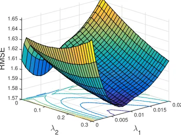
Figure 2: Average RMSE error on the test set of synthetic data for all tasks varying pa-rameters λ2 (controls sparsity on Ω) and λ1 (controls sparsity on W).
4.1.1 Synthetic Data set
We created a synthetic data set with 10 linear regression tasks of dimension D=Dr+Du,
where Dr and Du are the number of relevant and non-relevant (unnecessary) variables,
respectively. This is to evaluate the ability of the algorithm to discard non-relevant features. We usedDr= 30 andDu = 5. For each task, the relevant input variablesX0kare generated
i.i.d. from a multivariate normal distribution, X0k ∼ N(0,IDr). The corresponding output variable is generated as yk = X0kwk+ξ where ξi ∼ N(0,1),∀i = 1, ..., nk. Unnecessary
variables are generated as X00k ∼ N(0,IDu). Hence, the total synthetic input data of the
k-th task is formed as the concatenation of both set of variables, Xk = [X0k X00k]. Note
that only the relevant variables are used to produce the output variableyk. The parameter vectors for all tasks are chosen so that tasks 1 to 4 and 5 to 10 form two groups. Parameters for tasks 1-4 were generated as: wk =wabk+ξ, whereis the element-wise Hadamard
product; and for tasks 5-10: wk=wbbk+ξ, whereξ =N(0,0.2IDr). Vectorswaandwb are generated fromN(0,IDr), whilebk∼ U(0,1) are uniformly distributedDr-dimensional random vectors. In summary, we have two clusters of mutually related tasks. We train the
p-MSSL model with 50 data instances and test it on 100 data instances.
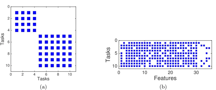
Figure 1 shows the RMSE error for p-MSSL and for the case where Ordinary Least Squares (OLS) was applied individually for each task. As expected, sharing information among related tasks improves prediction accuracy. p-MSSL does well on related tasks 1 to 4 and 5 to 10. Figures 3a and 3b depict the sparsity pattern of the task parametersW and the precision matrixΩ estimated by thep-MSSL algorithm. As can be seen, our model is able to recover the true dependence structure among tasks. The two clusters of tasks were clearly revealed, indicated by the filled squares, meaning non-zero entries in the precision matrix, and then, relationship among tasks. Additionally,p-MSSL was able to discard most of the irrelevant features (last five) intentionally added into the synthetic data set.
Tasks
0 2 4 6 8 10
Tasks
0
2
4
6
8
10
(a)
Features
0 10 20 30
Tasks
0
5
10
(b)
Figure 3: Sparsity pattern of the p-MSSL estimated parameters on the synthetic data set: (a) precision matrix Ω; (b) weight matrixW. The algorithm identified the true task relationship in (a) and removed most of the non-relevant features (last five columns) in (b).
data set. The best solution is with a sparse precision matrix, as we can see in Figure 2 (smallest RMSE with λ2 > 0). We should mention that as we increase λ1 we encourage sparsity on W and, as a consequence, it becomes harder for p-MSSL to capture the true relationship among the column vectors (tasks parameters), since it learns Ωfrom W. This drawback is overcome in ther-MSSL algorithm, in which the precision matrix is estimated from the residuals instead of being estimated from the task parameters directly.
4.1.2 Combining Earth System Models
An Earth System Model (ESM) is a complex mathematical representation of the major climate system components (atmosphere, land surface, ocean, and sea ice), and their in-teractions. They are run as computer simulations, to predict climate variables such as temperature, pressure, and precipitation over multiple centuries. Several ESMs have been proposed by climate science institutes from different countries around the world.
The forecasts of future climate variables as predicted by these models have high vari-ability, which in turn introduces uncertainty in analysis based on these predictions. One of the reasons for such uncertainty in the response of the ESMs comes from the model variability due to the fact that ESMs implements certain climatic process in different ways. Then, suitably combining outputs from multiple ESMs can greatly reduce the variability. Another equally important source of uncertainty is due to initial conditions. As ESMs are non-linear dynamic systems, changes in initial conditions can lead to different realizations of climate. In this work we focus only on the model variability. Modeling uncertainty from initial conditions is an ongoing work.
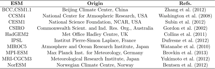
ESM Origin Refs. BCC CSM1.1 Beijing Climate Center, China Zhang et al. (2012)
CCSM4 National Center for Atmospheric Research, USA Washington et al. (2008) CESM1 National Science Foundation, NCAR, USA Subin et al. (2012) CSIRO Commonwealth Scient. and Ind. Res. Org., Australia Gordon et al. (2002) HadGEM2 Met Office Hadley Centre, UK Collins et al. (2011) IPSL Institut Pierre-Simon Laplace, France Dufresne et al. (2012) MIROC5 Atmosphere and Ocean Research Institute, Japan Watanabe et al. (2010) MPI-ESM Max Planck Inst. for Meteorology, Germany Brovkin et al. (2013) MRI-CGCM3 Meteorological Research Institute, Japan Yukimoto et al. (2012)
NorESM Norwegian Climate Centre, Norway Bentsen et al. (2012)
Table 1: Description of the Earth System Models used in the experiments.
Canada contrasts with the semi-arid climate in western United States and Mexico’s central area. The Rocky Mountains have a large impact in land’s climate, and temperature signifi-cantly varies due to topographic effects (elevation and slope) (Kinel et al., 2002). Southeast of the United States is characterized by its subtropical humid climate with relatively high temperatures and an evenly distributed precipitation throughout the year.
For the experiments we use 10 ESMs from the CMIP5 data set (Taylor et al., 2012). De-tails about the ESMs data sets are listed in Table 1. The global observation data for surface temperature is obtained from the Climate Research Unit (CRU) at the University of East Anglia. Both, ESM outputs and observed data are the raw temperatures (not anomalies) measured in degree Celsius. We align the data from the ESMs and CRU observations to have the same spatial and temporal resolution, using publicly available climate data opera-tors (CDO). For all the experiments, we used a 2.5o×2.5ogrid over latitudes and longitudes in South and North America, and monthly mean temperature data for 100 years, 1901-2000, with records starting from January 16, 1901. In other words, we have two data sets: (1) South America with 250 spatial locations; and (2) North America with 490 spatial locations over land. Data sets and code are available at: bitbucket.org/andreric/mssl-code. For the MTL framework, each geographical location represents a task (regression problem).
From an MTL perspective, the two data sets have different levels of difficulty. North America data set has almost twice the number of tasks as compared to South America, so that we discuss the performance of MSSL in problems with high number of tasks. It brings new challenges to MTL methods. On the other hand, South America has a more diverse cli-mate, which makes task dependence structure more complex. Preliminary results on South America were published in Gon¸calves et al. (2015) employing a high-level description format.
Baselines and Evaluation: We consider the following eight baselines for comparison and evaluation of MSSL performance for the ESM combination problem. The first two baselines (MMA and Best-ESM) are commonly used in climate sciences due to their stability and simple interpretation. We will refer to these baselines and MSSL as the “models” in the sequel and the constituent ESMs as “submodels”. Four well known MTL methods were also added in the comparison. The eight baselines are:
2. Best-ESM: uses the predicted outputs of the best ESM in the training phase (lowest RMSE). This baseline is not a combination of submodels, but a single ESM instead.
3. Ordinary Least Squares (OLS): performs an ordinary least squares regression for each geographic location, independently of the others.
4. Spatial Smoothing Multi Model Regression (S2M2R): proposed by Subbian and Banerjee (2013) to deal with ESM outputs combination, can be seen as a special case of MSSL with the pre-defined dependence matrixΩequal to the Laplacian matrix.
5. MTL-FEAT (Argyriou et al., 2007): all the tasks are assumed to be related and share a low-dimensional feature subspace. The following two methods, 6 and 7, can be seen as relaxations of this assumption. We used the code provided in MALSAR package (Zhou et al., 2011a).
6. Group-MTL (Kang et al., 2011): groups of related tasks are assumed and tasks be-longing to the same group share a common feature representation. The code was taken from the author’s homepage: http://www-scf.usc.edu/~zkang/GoupMTLCode.zip.
7. GO-MTL (Kumar and Daume III, 2012): founded on a relaxation of the group idea in Kang et al. (2011) by allowing subspaces shared by each group to overlap between them. We obtained the code directly from the authors.
8. MTRL (Zhang and Yeung, 2010): the covariance matrix among tasks coefficients is captured by imposing a matrix-variate normal prior over the coefficient matrix W. The non-convex MAP problem is relaxed and an alternating minimization procedure is proposed to solve the convex problem. The code was taken from author’s homepage:
http://www.comp.hkbu.edu.hk/~yuzhang/codes/MTRL.zip.
Methodology
We assume here that sub-models skills are stationary, that is, the coefficient associated with each sub-model does not change over time. To have an overall measure of the capa-bility of the method, we considered scenarios with different amount of data available for training. For each scenario, the same number of training data (columns of Table 2) are used for all tasks, and the remaining data is used for test. Starting from one year of temperature measures (12 samples), we increase till ten years of data for training. The remained data was used as test set. For each scenario 30 independent runs are performed. Therefore, the results are reported as the average and standard deviation of RMSE for all scenarios.
Results
Tasks
0 50 100 150 200 250
Tasks 0 50 100 150 200 250 Laplacian matrix South America Tasks
0 50 100 150 200 250
Tasks 0 50 100 150 200 250
Learned Precision matrix South America
Tasks 0 100 200 300 400
Tasks 0 50 100 150 200 250 300 350 400 450 Laplacian matrix North America Tasks 0 100 200 300 400
Tasks 0 50 100 150 200 250 300 350 400 450
Learned Precision matrix North America
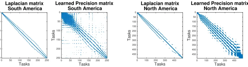
Figure 4: Laplacian matrix (on grid graph) assumed by S2M2R and the precision matrix learned by r-MSSLcop on both South and North America. r-MSSLcop can capture spatial relations beyond immediate neighbors. While South America is densely connected in the Amazon forest area (corresponding to top left corner) along with many spurious connections, North America is more spatially smooth.
precipitation and S2M2R may not succeed in those problems. On the other hand, MTL methods are general enough and in principle can be used for any climate variable. In the realm of MTL methods, all the four MSSL instantiations outperform the four other MTL contenders. It is worth observing that the two MSSL methods based on Gaussian Copula models provided smaller RMSE than the two with Gaussian models, particularly for problems with small training sample size. As Gaussian Copula models are more flexible, it is able to capture a wider range of task dependences than ordinary Gaussian models.
Similar behavior is observed in North America data set, except for the fact that MMA does much better than Best-ESM for all training sample settings. Again, all the four MSSL instantiations provided better future temperature projection. We also note that the residual-based structure dependence modeling with Gaussian Copula,r-MSSLcop, produced slightly better results than the other three MSSL instantiations. As will be left clear in Figures 4 and 6, residual-based MSSL coherently captures related geographical locations, indicating that it can be used as an alternative to parameter-based task dependence modeling.
Figure 4 shows the precision matrix estimated by the r-MSSLcop algorithm and the Laplacian matrix assumed by S2M2R in both South and North America. Blue dots means negative entries in the matrix, while red, positive. Interpreting the entries of the matrix in terms of partial correlation, Ωij <0 means positive partial correlation between wi and wj, while Ωij > 0 means negative partial correlation. Not only is the precision matrix
forr-MSSLcop able to capture the relationship among a geographical locations’ immediate neighbors (as in a grid graph) but it also recovers relationships between locations that are not immediate neighbors. The plots also provide an information of the range of neighborhood influence, which can be useful in spatial statistics analysis.
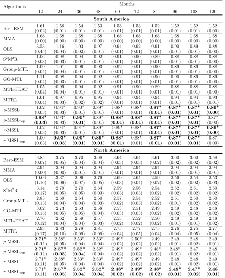
Algorithms Months
12 24 36 48 60 72 84 96 108 120
South America
Best-ESM 1.61 1.56 1.54 1.53 1.53 1.53 1.52 1.52 1.52 1.52
(0.02) (0.01) (0.01) (0.01) (0.01) (0.01) (0.01) (0.01) (0.01) (0.00)
MMA 1.68 1.68 1.68 1.68 1.68 1.68 1.68 1.68 1.68 1.68
(0.00) (0.00) (0.00) (0.00) (0.00) (0.00) (0.00) (0.00) (0.00) (0.00)
OLS 3.53 1.16 1.03 0.97 0.94 0.92 0.91 0.90 0.89 0.88
(0.45) (0.04) (0.02) (0.01) (0.01) (0.01) (0.01) (0.01) (0.01) (0.00)
S2M2R 1.06 0.98 0.94 0.92 0.91 0.90 0.89 0.88 0.88 0.88
(0.03) (0.03) (0.01) (0.01) (0.01) (0.01) (0.01) (0.01) (0.01) (0.00)
Group-MTL 1.09 1.01 0.96 0.93 0.92 0.91 0.90 0.89 0.89 0.88
(0.04) (0.04) (0.01) (0.01) (0.01) (0.01) (0.01) (0.01) (0.01) (0.00)
GO-MTL 1.11 0.98 0.94 0.92 0.92 0.91 0.90 0.90 0.89 0.89
(0.04) (0.03) (0.01) (0.01) (0.01) (0.01) (0.01) (0.01) (0.01) (0.00)
MTL-FEAT 1.05 0.99 0.94 0.92 0.91 0.90 0.89 0.88 0.88 0.88
(0.04) (0.04) (0.01) (0.01) (0.01) (0.01) (0.01) (0.01) (0.01) (0.00)
MTRL 1.01 0.97 0.95 0.95 0.94 0.94 0.94 0.94 0.94 0.93
(0.04) (0.03) (0.02) (0.02) (0.01) (0.01) (0.01) (0.01) (0.01) (0.01)
p-MSSL 1.02 0.94* 0.90* 0.89* 0.88* 0.88* 0.87* 0.87* 0.87* 0.86*
(0.03) (0.03) (0.01) (0.01) (0.01) (0.01) (0.01) (0.01) (0.01) (0.00)
p-MSSLcop 0.98* 0.93* 0.90* 0.89* 0.88* 0.88* 0.87* 0.87* 0.87* 0.87*
(0.03) (0.03) (0.01) (0.01) (0.01) (0.01) (0.01) (0.01) (0.01) (0.00)
r-MSSL 1.02 0.94* 0.91* 0.89* 0.89* 0.88* 0.87* 0.87* 0.87* 0.86*
(0.03) (0.03) (0.01) (0.01) (0.01) (0.01) (0.01) (0.01) (0.01) (0.00)
r-MSSLcop
1.00 0.93* 0.90* 0.89* 0.88* 0.88* 0.87* 0.87* 0.87* 0.87
(0.03) (0.03) (0.01) (0.01) (0.01) (0.01) (0.01) (0.01) (0.01) (0.00)
North America
Best-ESM 3.85 3.75 3.70 3.68 3.64 3.64 3.61 3.60 3.60 3.58
(0.07) (0.05) (0.04) (0.04) (0.03) (0.03) (0.02) (0.02) (0.02) (0.02)
MMA 2.94 2.94 2.94 2.94 2.94 2.94 2.94 2.94 2.94 2.94
(0.00) (0.00) (0.01) (0.01) (0.01) (0.01) (0.01) (0.01) (0.01) (0.01)
OLS 10.06 3.37 2.96 2.79 2.69 2.64 2.59 2.56 2.54 2.53
(1.16) (0.09) (0.07) (0.05) (0.03) (0.04) (0.02) (0.02) (0.02) (0.03)
S2M2R 3.14 2.79 2.70 2.64 2.59 2.56 2.54 2.52 2.51 2.50
(0.17) (0.05) (0.05) (0.03) (0.03) (0.03) (0.02) (0.02) (0.02) (0.02)
Group-MTL 2.83 2.69 2.64 2.60 2.57 2.54 2.52 2.51 2.50 2.50
(0.13) (0.04) (0.04) (0.03) (0.02) (0.03) (0.02) (0.01) (0.02) (0.02)
GO-MTL 3.02 2.73 2.63 2.58 2.53 2.51 2.49 2.49 2.48 2.48
(0.15) (0.05) (0.05) (0.04) (0.03) (0.03) (0.02) (0.02) (0.02) (0.02)
MTL-FEAT 2.76 2.62 2.59 2.57 2.53 2.52 2.50 2.49 2.49 2.48
(0.12) (0.04) (0.04) (0.03) (0.02) (0.02) (0.02) (0.01) (0.01) (0.02)
MTRL 2.93 2.83 2.78 2.81 2.75 2.77 2.75 2.76 2.75 2.77
(0.17) (0.10) (0.09) (0.09) (0.04) (0.05) (0.04) (0.04) (0.05) (0.04)
p-MSSL 2.71* 2.58* 2.53* 2.53* 2.49* 2.50* 2.49 2.49 2.48 2.49
(0.11) (0.05) (0.04) (0.04) (0.02) (0.02) (0.02) (0.01) (0.02) (0.01)
p-MSSLcop 2.71* 2.57* 2.52* 2.52* 2.49* 2.49* 2.48* 2.48* 2.47 2.48
(0.11) (0.05) (0.04) (0.04) (0.02) (0.02) (0.02) (0.01) (0.02) (0.01)
r-MSSL 2.71* 2.58* 2.53* 2.53* 2.49* 2.49* 2.49 2.48 2.48 2.49
(0.11) (0.05) (0.04) (0.04) (0.02) (0.02) (0.02) (0.01) (0.02) (0.01)
r-MSSLcop
2.71* 2.57* 2.52* 2.52* 2.48* 2.49* 2.48* 2.48* 2.47* 2.48
(0.11) (0.05) (0.04) (0.04) (0.02) (0.02) (0.02) (0.01) (0.02) (0.01)
Table 2: Mean and standard deviation over 30 independent runs for several amounts of monthly data used for training. The symbol ”∗” indicates statistically significant (t-test, P
60° S 40° S 20° S 0° MMA: Average RMSE=1.68 0 0.5 1 1.5 2
60° S 40° S 20° S 0° Best ESM: Average RMSE=1.53 0 0.5 1 1.5 2
60° S 40° S 20° S 0° OLS: Average RMSE=0.94 0 0.5 1 1.5 2
60° S 40° S 20° S 0° r−MSSLcop: Average RMSE=0.90 0 0.5 1 1.5 2 30 ° N 60 ° N MMA: Average RMSE=2.94 0 0.5 1 1.5 2 2.5 3 3.5 4 30 ° N 60 ° N Best ESM: Average RMSE=3.64 0 0.5 1 1.5 2 2.5 3 3.5 4 30 ° N 60 ° N OLS: Average RMSE=2.69 0 0.5 1 1.5 2 2.5 3 3.5 4 30 ° N 60 ° N r−MSSLcop: Average RMSE=2.48 0 0.5 1 1.5 2 2.5 3 3.5 4
Figure 5: [Best viewed in color] RMSE per location forr-MSSLcopand three common meth-ods in climate sciences, computed using 60 monthly temperature measures for training. It shows thatr-MSSLcopsubstantially reduces RMSE, particularly in Northern South America and Northwestern North America.
performs better because it learns a more appropriate weight combination on the model outputs and incorporates spatial smoothing by learning the task relationship.
Figure 6 presents the dependence structure estimated byr-MSSLcopfor South and North America data sets. Blue connections indicate dependent regions.
We immediately observe that locations in the northwest part of South America are densely connected. This area has a typical tropical climate and comprises the Amazon rainforest which is known for having hot and humid climate throughout the year with low temperature variation (Ramos, 2014). The cold climates which occur in the southernmost parts of Argentina and Chile are clearly highlighted. Such areas have low temperatures throughout the year, but there are large daily variations (Ramos, 2014). An important observation can be made about South America west cost, ranging from central Chile to Venezuela passing through Peru which has one of the driest deserts in the world. These areas are located to the left side of Andes Mountains and are known for arid climate. The average model is not performing well on this region compared to r-MSSLcop. We can see the long lines connecting these coastal regions, which probably explains the improvement in terms of RMSE reduction achieved byr-MSSLcop. The algorithm uses information from related locations to enhance its performance on these areas.
South America
● ●
● ●
● ● ●
● ● ●
● ● ●
● ● ● ●
● ● ● ● ●
● ● ● ● ● ● ●
● ● ● ● ● ● ●
● ● ● ● ● ● ●
● ● ● ● ● ● ● ●
● ● ● ● ● ● ● ● ●
● ● ● ● ● ● ● ● ●
● ● ● ● ● ● ● ● ● ● ● ●
● ● ● ● ● ● ● ● ● ● ● ●
● ● ● ● ● ● ● ● ● ● ● ● ●
● ● ● ● ● ● ● ● ● ● ● ● ● ● ●
● ● ● ● ● ● ● ● ● ● ● ● ● ● ●
● ● ● ● ● ● ● ● ● ● ● ● ● ● ● ● ●
● ● ● ● ● ● ● ● ● ● ● ● ● ● ● ● ● ●
● ● ● ● ● ● ● ● ● ● ● ● ● ● ● ● ● ●
● ● ● ● ● ● ● ● ● ● ● ● ● ● ●
● ● ● ● ● ● ● ● ● ● ● ● ●
● ● ● ● ● ● ● ● ● ● ●
● ● ● ● ● ● ● ● ●
● ● ● ● ● ● ● ●
● ● ● ● ●
North America
●
●●●●
●●●● ●
●●●
●●●●
●●●●●●● ●
●●●●●●●●●● ● ●●
●●●●●●●●●● ●●●●
●●●●●●●●●●●● ●●●●●●
●●●●●●●●●●●● ●●●●●●
● ●●●●●●●●●●●● ●●●●●●●
● ●●●●●●●●●●●● ●●●●●●●●
● ●●●●●●●●●●●● ●●●●●●●●●●●●
● ●●●●●●●●●●●● ●●●●●●●●●●● ●
●● ●●●●●●●●●●●● ●●●●●●●●●● ●
●●● ●●●●●●●●●●●● ●●●● ●●●●●●● ●●
●●●●● ●●●●●●●●●●●● ●●●● ●●●●●●● ●
● ● ●●●●●● ●●●●●●●●●●● ●●●●●●
●●●● ● ●●●●●●●● ●●●●●●●●●●● ●●●●
●●●●●● ●●●●●●●●●●● ●●●●●●●●●●●● ● ●
●●●●●●● ●●●●●●●●●●● ●●●●●●●●●●●● ●●● ●●●●●
●●●●●● ●●●●●●●●●●● ●●●●●●●●●●●● ● ●● ●●●●
●●●●● ● ●● ●●●●●● ●● ●●●●●●●
● ●●●●●● ●●● ●●●●●
●●● ● ● ●●●●●
● ● ●●●●
● ●● ● ●●●●●●
●●●●●●●
Figure 6: Relationships between geographical locations estimated by the r-MSSLcop al-gorithm using 120 months of data for training. The blue lines indicate that connected locations are conditionally dependent on each other. As expected, temperature is very spa-tially smooth, as we can see by the high neighborhood connectivity, although some long range connections are also observed.
surface temperature in these area (Twilley, 2001), that in turn has a strong impact on Gulf of Mexico costal regions.
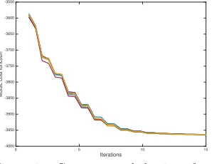
4.1.3 MSSL sensitivity to initial values of W
As discussed earlier, the MSSL algorithms may be susceptible to the choice of initial values of the parameters Ω and W, as the optimization function (3) is not jointly convex on Ω
and W. In this section we analyze the impact of different parameter initializations on the RMSE and the number of non-zero entries in the estimated Ωand W parameters.
Table 3 shows the mean and standard deviation over 10 independent runs with random initialization of W in the interval [-0.5,0.5] for the South America data set. For the Ω
matrix we started with an identity matrix, as it is reasonable to assume tasks independence beforehand. The results showed that the solutions are not sensitive to initial values of
Synt. South North
America America
RMSE 1.14 (2e-6) 0.86 (0) 2.46 (1.6e-4) # nzW 345 (0) 2341 (0.32) 4758 (2.87)
# nzΩ 55(0) 4954 (0.63) 73520 (504.4)
Table 3: p-MSSL sensitivity to initial values of W in terms of RMSE, mean and standard deviation, and num-ber of non-zero entries inWandΩ.
Iterations
0 5 10 15
MSSL cost function
-4000 -3950 -3900 -3850 -3800 -3750 -3700 -3650 -3600 -3550
Figure 7: Convergence behavior of p -MSSL for distinct initializations of the weight matrixW.
4.2 Classification
We test the performance of the p-MSSL on five data sets (six problems) described below. Recall thatr-MSSL can not be applied for classification problems, once it relies on a Gaus-sian assumption of the residuals. This is currently the subject of an ongoing work. All data sets were standardized, then all features have zero mean and standard deviation one.
• Landmine Detection: Data from 19 landmine fields were collected, which have dis-tinct characteristics. Each object in a given data set is represented by a 9-dimensional feature vector and the corresponding binary label (1 for landmine and 0 for clutter) (Xue et al., 2007). The feature vectors are extracted from radar images, concatenating four moment-based features, three correlation-based features, one energy ratio feature and one spatial variance feature. The goal is to classify between mine or clutter.
• Spam Detection: E-mail spam data set from ECML 2006 discovery challenge. It consists of two problems: Problem A with e-mails from 3 different users (2500 e-mails per user); and Problem B with e-mails from 15 distinct users (400 e-mails per user). We performed feature selection to get the 500 most informative variables using the Laplacian score feature selection algorithm (He et al., 2006). The goal is to classify between spam vs. ham. For both problems, we create different tasks for different users. This data set can be found athttp://www.ecmlpkdd2006.org/challenge.html.
• MNISTdata set consists of 28×28-size images of hand-written digits from 0 through 9. We transform this multiclass classification problem by applying the all-versus-all decomposition, leading to 45 binary classification problems (tasks). When a new test sample arrives, a voting scheme is performed among the classifiers. The number of samples for each classification problem is about 15000. This data set can be found at
http://yann.lecun.com/exdb/mnist/.
• Yale-faces: The face recognition data set contains 165 grayscale images with dimen-sion 32x32 pixels of 15 individuals. Similar to MNIST, the problem is also trans-formed by all-versus-all decomposition, totalling 105 binary classification problems (tasks). For each task only 22 samples are available. This data set can be found at
http://vision.ucsd.edu/content/yale-face-database.
Baseline algorithms: Four baseline algorithms were considered in the experiments and the regularization parameters for all algorithms were selected using cross-validation from the set {0.01, 0.1, 1, 10, 100}. The algorithms are:
1. Logistic Regression (LR): learns separate logistic regression models for each task.
2. MTL-FEAT (Argyriou et al., 2007): employs an `2,1-norm regularization term to
capture the task relationship from multiple related tasks constraining all models to share a common set of features.
3. CMTL(Zhou et al., 2011b): incorporates a regularization term to induce clustering between tasks and then share information only to tasks belonging to the same cluster.
4. Low rank MTL (Abernethy et al., 2006): assumes that related tasks share a low dimensional subspace and applies a trace regularization norm to capture that relation.
Results: Table 4 shows the results of each algorithm for all data sets. It was obtained over 10 independent runs using a holdout cross-validation (2/3 for training and 1/3 for test). The performance of each run is measured by the average of the performance of all tasks.
Algorithms Landmine Spam Spam MNIST Letter Yale
3-users 15-users faces
LR 6.01 6.62 16.46 9.80 5.56 26.04
(0.37) (0.99) (0.67) (0.19) (0.19) (1.26)
CMTL 5.98 3.93 8.01 2.06 8.22 9.43
(0.32) (0.45) (0.75) (0.14) (0.25) (0.78)
MTL-FEAT 6.16 3.33 7.03 2.61 11.66 7.15
(0.31) (0.43) (0.67) (0.08) (0.29) (1.60)
Trace 5.75 2.65 5.40 2.27 5.90 7.49
(0.28) (0.32) (0.54) (0.09) (0.21) (1.72)
p-MSSL 5.68 1.90* 6.55 1.96* 5.34* 9.58
(0.37) (0.27) (0.68) (0.08) (0.19) (0.91)
p-MSSLcop 5.68 1.77* 5.32 1.95* 5.29* 5.28*
(0.35) (0.29) (0.45) (0.08) (0.19) (0.45)
Table 4: Average classification error rates and standard deviation over 10 independent runs for all methods and data sets considered. Bold values indicate the best value and the symbol “*” means significant statistical improvement of the MSSL algorithm in relation to the contenders determined by t-test with P<0.05.
![Figure 5: [Best viewed in color] RMSE per location for rods in climate sciences, computed using 60 monthly temperature measures for training](https://thumb-us.123doks.com/thumbv2/123dok_us/9792806.1965052/22.612.100.520.95.266/figure-location-climate-sciences-computed-temperature-measures-training.webp)