Journal of Machine Learning Research 17 (2016) 1-61 Submitted 6/14; Revised 7/15; Published 6/16
How to Center Deep Boltzmann Machines
Jan Melchior [email protected]
Asja Fischer [email protected]
Laurenz Wiskott [email protected]
Institut f¨ur Neuroinformatik Ruhr-Universit¨at Bochum Bochum, D-44801, Germany
Editor:Yoshua Bengio
Abstract
This work analyzes centered Restricted Boltzmann Machines (RBMs) and centered Deep Boltzmann Machines (DBMs), where centering is done by subtracting offset values from visible and hidden variables. We show analytically that (i) centered and normal Boltz-mann Machines (BMs) and thus RBMs and DBMs are different parameterizations of the same model class, such that any normal BM/RBM/DBM can be transformed to an
equiv-alent centered BM/RBM/DBM and vice versa, and that this equivalence generalizes to
artificial neural networks in general, (ii) the expected performance of centered binary BMs/RBMs/DBMs is invariant under simultaneous flip of data and offsets, for any off-set value in the range of zero to one, (iii) centering can be reformulated as a different update rule for normal BMs/RBMs/DBMs, and (iv) using the enhanced gradient is equiv-alent to setting the offset values to the average over model and data mean. Furthermore, we present numerical simulations suggesting that (i) optimal generative performance is achieved by subtracting mean values from visible as well as hidden variables, (ii) centered binary RBMs/DBMs reach significantly higher log-likelihood values than normal binary RBMs/DBMs, (iii) centering variants whose offsets depend on the model mean, like the enhanced gradient, suffer from severe divergence problems, (iv) learning is stabilized if an exponentially moving average over the batch means is used for the offset values instead of the current batch mean, which also prevents the enhanced gradient from severe divergence, (v) on a similar level of log-likelihood values centered binary RBMs/DBMs have smaller weights and bigger bias parameters than normal binary RBMs/DBMs, (vi) centering leads to an update direction that is closer to the natural gradient, which is extremely efficient for training as we show for small binary RBMs, (vii) centering eliminates the need for greedy layer-wise pre-training of DBMs, which often even deteriorates the results independently of whether centering is used or not, and (ix) centering is also beneficial for auto encoders.
Keywords: centering, restricted Boltzmann machine, deep Boltzmann machine, gener-ative model, artificial neural network, auto encoder, enhanced gradient, natural gradient, stochastic maximum likelihood, contrastive divergence, parallel tempering
1. Introduction
In the last decade Restricted Boltzmann Machines (RBMs) got into the focus of attention because they can be considered as building blocks of deep neural networks (Hinton et al., 2006; Bengio, 2009). RBM training methods are usually based on gradient ascent on the
c
melchior, fischer and wiskott
Log-Likelihood (LL) of the model parameters given the training data. Since the gradient is intractable, it is often approximated using Gibbs sampling with only a few steps (Hinton et al., 2006; Tieleman, 2008; Tieleman and Hinton, 2009). Two major problems have been reported when training RBMs.
Firstly, the bias of the gradient approximation introduced by using only a few steps of Gibbs sampling may lead to a divergence of the LL during training (Fischer and Igel, 2010; Schulz et al., 2010; Fischer and Igel, 2011). To overcome the divergence problem Desjardins et al. (2010) and Cho et al. (2010) have proposed to use parallel tempering (Swendsen and Wang, 1986), which is an advanced sampling method that leads to a faster mixing Markov chain and thus to a better approximation of the LL gradient.
Secondly, the learning process is not invariant to the data representation. For example training an RBM on the MNIST data set leads to a better model than training it on 1-MNIST (the data set generated by flipping each bit in MNIST). This is due to missing invariance properties of the gradient with respect to these flip transformations and not due to the model’s capacity, since an RBM trained onMNIST can be transformed in such a way that it models1-MNIST with the same LL. Recently, two approaches have been introduced that address this invariance problem. The enhanced gradient (Cho et al., 2011, 2013b) has been designed as an invariant alternative to the true LL gradient of binary RBMs and has been derived by calculating a weighted average over the gradients one gets by applying any possible bit flip combination on the data set. Empirical results suggest that the enhanced gradient leads to more distinct features and thus to better classification results based on the learned hidden representation of the data. Furthermore, in combination with an adaptive learning rate the enhanced gradient leads to more stable training in the sense that good LL values are reached independently of the initial learning rate. Tang and Sutskever (2011) on the other hand have shown empirically that subtracting the data mean from the visible variables leads to a model that can reach similar LL values on theMNIST and the1-MNIST
data set and comparable results to those of the enhanced gradient.1 Removing the mean from all variables is known as the ‘centering trick’, which was originally proposed for feed forward neural networks (LeCun et al., 1998; Schraudolph, 1998). It has recently also been applied to the visible and hidden variables of Deep Boltzmann Machines (DBM) (Montavon and M¨uller, 2012) where it has been shown to lead to a better conditioned optimization problem. Furthermore, the learned features have shown better discriminative properties and centering has improved the generative properties of locally connected DBMs. A related approach applicable to multi-layer perceptrons where the activation functions of the neurons are transformed to have zero mean and zero slope on average has been proposed by Raiko et al. (2012). The authors could show that the gradient under this transformation gets closer to the natural gradient, which is desirable since the natural gradient follows the direction of steepest ascent in the manifold of probability distributions. Furthermore, the natural gradient is independent of the concrete parameterization of the distributions and is thus clearly the update direction of choice (Amari, 1998). Since the exact natural gradient is intractable already for rather small RBMs, Schwehn (2010) and Ollivier et al. (2011) have trained binary RBMs and Desjardins et al. (2013) binary DBMs using approximations of the natural gradient obtained by Markov chain Monte Carlo methods. However, due to
1. Note that changing the model such that the mean of the visible variables is removed is not equivalent to just removing the mean of the data.
How to Center Deep Boltzmann Machines
the computational overhead the practical relevance of the natural gradient for RBM/DBM training remains questionable. Another approach related to the centering trick is batch normalization, which has recently been proposed by Ioffe and Szegedy (2015) and aims at removing first and second order statistics of the pre synaptic activation in a feed forward network.
In this article2 we give a unified view on centering, revealing that the methods proposed by Cho et al. (2011), Tang and Sutskever (2011), and Montavon and M¨uller (2012) can all be considered as different ways of applying the centering trick to RBMs and DBMs. Furthermore, we analyze the properties and performance of different centering variants. In Section 2, we begin with a brief overview over binary RBMs, the standard learning algorithms, the natural gradient of the LL of RBMs, and the basic ideas used to construct the enhanced gradient. In Section 3, we discuss the theoretical properties of centered RBMs, show that centering can be reformulated as a different update rule for normal RBMs, that the enhanced gradient is a particular form of centering, and finally that centering and its properties naturally extend to DBMs and BMs. Furthermore, in Section 4, we show that centering is an alternative parameterization for arbitrary Artificial Neural Networks (ANNs) in general and we discuss how the parameters of centered and normal ANNs should be initialized. Our experimental setups are described in Section 5 before we empirically analyze the performance of centered RBMs with different initializations, offset parameters, sampling methods, and learning rates in Section 6. This empirical analysis includes a comparison of the centered gradient with the natural gradient and extensive experiments on 10 real world data sets. In addition we have also performed experiments with DBMs and Auto encoders (AEs) on the 10 real work data sets. Finally our work is concluded in Section 7.
2. Restricted Boltzmann Machines
An RBM (Smolensky, 1986) is a bipartite undirected graphical model with a set ofN visible and M hidden variables taking values x = (x1, ..., xN) and h = (h1, ..., hM), respectively. Since an RBM is a Markov random field, its joint probability distribution is given by a Gibbs distribution
p(x,h) = 1
Ze
−E(x,h) ,
with partition functionZ and energyE(x,h). For binary RBMs,x∈ {0,1}N ,h∈ {0,1}M, the energy, which defines the bipartite structure, is given by
E(x,h) = −xTb−cTh−xTWh ,
where the weight matrixW, the visible bias vectorb, and the hidden bias vectorcare the parameters of the model, jointly denoted byθ. The partition function, which sums over all possible visible and hidden states, is given by
Z = X
x
X
h
e−E(x,h) .
2. Previous versions of this work have been published as an eprint (Melchior et al., 2013) and as part of the PhD thesis by Fischer (2014).
melchior, fischer and wiskott
RBM training is usually based on gradient ascent using approximations of the LL gradient
∇θ = ∂hlog (p(x|θ))id
∂θ =−
∂E(x,h)
∂θ
d +
∂E(x,h)
∂θ
m
,
where h·im is the expectation under p(x,h) and h·id is the expectation under p(h|x)pe(x) with empirical distribution pe. We use the notation ∇θ for the derivative of the LL with respect to θ in order to be consistent with the notation used by Cho et al. (2011). For binary RBMs the gradient becomes
∇W = hxhTid− hxhTim ,
∇b = hxid− hxim , ∇c = hhid− hhim .
Common RBM training methods approximateh·im by samples gained by different Markov chain Monte Carlo methods. Sampling k (usually k = 1) steps from a Gibbs chain ini-tialized with a data sample yields Contrastive Divergence (CD) (Hinton et al., 2006). In stochastic maximum likelihood (Younes, 1991), in the context of RBMs also known as Per-sistent Contrastive Divergence (PCD) (Tieleman, 2008), the chain is not reinitialized with a data sample after parameter updates. This has been reported to lead to better gradient approximations if the learning rate is chosen sufficiently small. Fast Persistent Contrastive Divergence (FPCD) (Tieleman and Hinton, 2009) tries to further speed up learning by introducing an additional set of parameters, that is only used for Gibbs sampling during learning. The advanced sampling method Parallel Tempering (PT) (Swendsen and Wang, 1986) introduces additional ‘tempered’ Gibbs chains corresponding to smoothed versions of p(x,h). The energy of these distributions is multiplied by T1, where T is referred to as temperature. The higher the temperature of a chain, the ‘smoother’ the correspond-ing distribution and the faster the chain mixes. Samples may swap between chains with a probability given by the Metropolis Hastings ratio, which leads to better mixing of the original chain with temperature T = 1 (a first theoretical analysis of the mixing rate of PT for sampling in RBMs has been given by Fischer and Igel, 2015). We use PTcto denote the RBM training algorithm that uses Parallel Tempering withctempered chains as a sampling method. Usually only one step of Gibbs sampling is performed in each tempered chain be-fore allowing samples to swap, and a deterministic even odd algorithm (Lingenheil et al., 2009) is used as a swapping schedule. PTcincreases the mixing rate and has been reported to achieve better gradient approximations than CD and (F)PCD (Desjardins et al., 2010; Cho et al., 2010) with the drawback of having a higher computational cost.
See the introductory paper of Fischer and Igel (2014) for a recent review of RBMs and their training algorithms.
2.1 Enhanced Gradient
Cho et al. (2011) have proposed a different way to update parameters during training of binary RBMs, which is invariant to the data representation.
When transforming the state (x,h) of a binary RBM by flipping some of its variables (that is ˜xi = 1−xi, and ˜hj = 1−hj for some i, j), yielding a new state (˜x,h˜), one can
How to Center Deep Boltzmann Machines
transform the parameters θ of the RBM to θ˜such thatE(x,h|θ) =E(˜x,h˜|θ˜) +const and thusp(x,h|θ) =p(˜x,˜h|θ˜). However, if we update the parameters of the transformed model
based on the corresponding LL gradient toθ˜0 =θ˜+η∇θ˜and apply the inverse parameter
transformation to θ˜0, the result differs from θ0 = θ +η∇θ. The described procedure of transforming, updating, and transforming back can be regarded as a different way to updateθ.
Following this line of thought there exist 2N+M different parameter updates correspond-ing to the 2N+M possible binary flips of (x,h). Cho et al. (2011) have proposed the en-hanced gradient as a weighted sum of these 2N+M parameter updates, which for their choice of weighting is given by
∇eW = h(x− hxid)(h− hhid)Tid− h(x− hxim)(h− hhim)Tim , (1)
∇eb = hxid− hxim− ∇eW 1
2(hhid+hhim) , (2)
∇ec = hhid− hhim− ∇eWT1
2(hxid+hxim) . (3)
It has been shown that the enhanced gradient is invariant to arbitrary bit flips of the vari-ables and therefore invariant under the data representation, which has been demonstrated on theMNIST and1-MNIST data set. Furthermore, the authors have reported more stable training under various settings in terms of the LL estimate and classification accuracy.
2.2 Natural Gradient
Following the direction of steepest ascent in the Euclidean parameter space (as given by the standard gradient) does not necessarily correspond to the direction of steepest ascent in the manifold of probability distributions {p(x|θ),θ ∈Θ}, which we are actually interested in. To account for the local geometry of the manifold, the Euclidean metric should be replaced by the Fisher information metric defined by ||θ||I(θ) =pPθkIkl(θ)θl, where I(θ) is the Fisher information matrix (Amari, 1998). Thekl-th entry of the Fisher information matrix for a parameterized distributionp(x|θ) is given by
Ikl(θ) =
∂log (p(x|θ))
∂θk
∂log (p(x|θ))
∂θl
m
,
whereh·im denotes the expectation under p(x|θ). The gradient associated with the Fisher metric is called the natural gradient and is given by
∇nθ = I(θ)−1∇θ .
The inverse Fisher information matrix corrects the direction and length of the standard gra-dient to achieve the largest change of the objective function (here the LL) for an infinitesimal small stepδθfromp(x|θ) top(x|θ+δθ) in terms of the Kullback-Leibler divergence (Amari, 1998). This makes the natural gradient independent of the parameterization leading to an invariance to arbitrary coordinate transformations such as flipping variables, which makes it clearly the update direction of choice.
melchior, fischer and wiskott
For binary RBMs the entries of the Fisher information matrix (Amari et al., 1992; Desjardins et al., 2013; Ollivier et al., 2011) are given by
Iwij,wuv(θ) =I,wuv,wij(θ) = hxihjxuhvim− hxuhvimhxuhvim = Covm(xihj, xuhv) ,
Iwij,bu(θ) =Ibu,wij(θ) = Covm(xihj, xu) ,
Iwij,cv(θ) =Icv,wij(θ) = Covm(xihj, hv) ,
Ibi,bu(θ) =Ibu,bi(θ) = Covm(xi, xu) ,
Icj,cv(θ) =Icv,cj(θ) = Covm(hj, hv) ,
whereCovm(·,·) denotes the covariance under the model distribution. Since these expres-sions involve expectations under the model distribution they are not tractable in general, but can be approximated using MCMC methods (Ollivier et al., 2011; Desjardins et al., 2013). Furthermore, a diagonal approximation of the Fisher information matrix could be used. However, the approximation of the natural gradient for RBMs and DBMs is still com-putationally very expensive so that the practical usability remains questionable (Schwehn, 2010; Ollivier et al., 2011; Desjardins et al., 2013).
3. Centered Restricted Boltzmann Machines
Inspired by the centering trick proposed by LeCun et al. (1998), Tang and Sutskever (2011) have addressed the problem that RBMs perform differently on the MNIST and 1-MNIST
data set by changing the energy of the RBM in a way that the mean of the input data is removed. Montavon and M¨uller (2012) have extended the idea of centering to the visible and hidden variables of DBMs and have shown that centering improves the conditioning of the underlying optimization problem, leading to models with better discriminative properties for DBMs in general and better generative properties in the case of locally connected DBMs. Following their line of thought, the energy for a centered binary RBM where the visible and hidden variables are shifted by the offset parameters µ = (µ1, . . . , µN) and
λ= (λ1, . . . , λM), respectively, can be formulated as
E(x,h) = −(x−µ)Tb−cT (h−λ)−(x−µ)T W(h−λ) . (4)
By setting both offsets to zero one retains the normal binary RBM. Setting µ=hxid and
λ=0leads to the model introduced by Tang and Sutskever (2011), and by settingµ=hxid
and λ = hhid we get a shallow variant of the centered DBM analyzed by Montavon and M¨uller (2012).
The conditional probabilities for a variable taking the value one are given by
p(xi = 1|h) = σ(wi∗(h−λ) +bi) , (5)
p(hj = 1|x) = σ((x−µ)T w∗j+cj) , (6)
whereσ(·) is the sigmoid function, wi∗ represents the ith row, and w∗j the jth column of
the weight matrixW. The LL gradient now takes the form
∇W = h(x−µ)(h−λ)Tid− h(x−µ)(h−λ)Tim , (7)
∇b = hx−µid− hx−µim = hxid− hxim , (8)
∇c = hh−λid− hh−λim = hhid− hhim . (9)
How to Center Deep Boltzmann Machines
∇band∇care independent of the choice of µand λand thus centering only affects∇W. It can be shown (see Appendix A) that the gradient of a centered BM is invariant to flip transformations if a flip ofxi to 1−xi implies a change of µi to 1−µi, and in the case of RBMs a fliphj to 1−hj implies a change ofλj to 1−λj. This holds forµi = 0.5,λj = 0.5 but remarkably also for the expectation values overxiandhj under any distribution. Moreover, if the offsets are set to the expectation values, centered RBMs get also invariant to shifts
Algorithm 1:Training centered RBMs
1 Initialize W ; /* i.e., W← N(0,0.01)N×M */ 2 Initialize µ,λ; /* i.e., µ← hdatai,λ←0.5 */ 3 Initialize b,c; /* i.e., b←σ−1(µ),c←σ−1(λ) */ 4 Initialize η, νµ, νλ ; /* i. e., η, νµ, νλ∈ {0.001, ...,0.1} */ 5 repeat
6 foreachbatchindatado
7 foreachsamplexd inbatchdo
8 Calculatehd=p(h=1|xd) ; /* . Eq. (6) */ 9 Samplexm f rom RBM ; /* i.e., PCD-1, . Eqs. (5), (6) */ 10 Calculatehm =p(h=1|xm) ; /* . Eq. (6) */ 11 Store xm,hd,hm
12 Estimateµbatch; /* i.e. µbatch← hxdi */ 13 Estimateλbatch ; /* i.e. λbatch← hhdi */
/* Transform parameters with respect to the new offsets */
14 b←b+νλW(λbatch−λ) ; /* . Eq. (11), λ˜= (1−νλ)λ+νλλbatch */
15 c←c+νµWT (µbatch−µ) ; /* . Eq. (12), µ˜ = (1−νµ)µ+νµµbatch */
/* Update offsets using exp. moving average with sliding factors
νµ and νλ */
16 µ←(1−νµ)µ+νµµbatch
17 λ←(1−νλ)λ+νλλbatch
/* Update parameters using the gradient with learning rate η */
18 ∇W ← h(xd−µ)(hd−λ)Ti − h(xm−µ)(hm−λ)Ti ; /* . Eq. (7) */
19 ∇b← hxdi − hxmi ; /* . Eq. (8) */
20 ∇c← hhdi − hhmi ; /* . Eq. (9) */
21 W←W+η∇W
22 b←b+η∇b
23 c←c+η∇c
24 until stopping criteria is met;
/* Transform network to a normal binary RBM if desired */
25 b←b−Wλ ; /* . Eq. (11) */
26 c←c−WTµ; /* . Eq. (12) */
27 µ←0
28 λ←0
melchior, fischer and wiskott
of variables (see Section 4). Note that these properties of centered RBMs naturally extend to centered BMs and DBMs (see Section 3.2, Appendix A and B).
If we set µ and λ to the expectation values of the variables, these values may depend on the RBM parameters (think for example about hhid) and thus they might change dur-ing traindur-ing. Consequently, a learndur-ing algorithm for centered RBMs needs to update the offset values to match the expectations under the distribution that has changed through a parameter update. When updating the offsets one needs to transform the RBM parameters such that the modeled probability distribution stays the same. An RBM with offsetsµand
λcan be transformed to an RBM with offsets µ˜ and λ˜ by
˜
W = W , (10)
˜
b = b+W˜λ−λ , (11)
˜c = c+WT (µ˜−µ) , (12)
such that E(x,h|θ,µ,λ) = E(x,h|θ˜,µ˜,λ˜) +const, is guaranteed (see Appendix B for a derivation for a more general BM). Obviously, this can also be used to transform a centered RBM to a normal RBM and vice versa, highlighting that centered and normal RBMs are just different parameterizations of the same model class.
If the intractable model mean is used for an offset, it has to be approximated by samples. Furthermore, when λ is chosen to be hhid or hhim or when µ is chosen to be hxim one could approximate the mean values either using the sampled states or the corresponding conditional probabilities. But due to the Rao-Blackwell theorem an estimation based on the probabilities has lower variance and therefore is the approximation of choice.3
Algorithm 1 shows pseudo code for training a centered binary RBM, where we use h·i to denote the average over samples from the current batch. Thus, for example, we write hxdi for the average value of data samples xd in the current batch, which is used as an approximation for the expectation ofxunder the data distribution, that ishxid. Similarly, hhdi =hp(h=1|xd)i approximateshhid, where p(x=1|h) denotes the vector containing the elementsp(xi = 1|h). Note that in Algorithm 1 the update of the offsets is performed before the gradient is calculated, such that gradient and reparameterization both use the current samples. This is in contrast to the algorithm for centered DBMs proposed by Montavon and M¨uller (2012), where the update of the offsets and the reparameterization follows after the gradient update. Thus, while the gradient still uses the current samples the reparameterization is based on samples gained from the model of the previous iteration. However, the proposed DBM algorithm smooths the offset estimations by an exponentially moving average over the sample means from many iterations, so that the choice of the sample set used for the offset estimation should be less relevant.
In Algorithm 1 an exponentially moving average for the approximation of µis obtained if the corresponding sliding factorνµ is set to 0< νµ<1 or prevented ifνµ= 1 and equiv-alently for λ and νλ. The effects of using an exponentially moving average are empirically analyzed in Section 6.5.
3. This can be proven analogously to the proof of proposition 1 in the work of Swersky et al. (2010).
How to Center Deep Boltzmann Machines
3.1 Centered Gradient
We now use the centering trick to derive a centered parameter update, which can replace the gradient during the training of normal RBMs. Similar to the derivation of the enhanced gradient we can transform a normal RBM to a centered RBM, perform a gradient update, and transform the RBM back (see Appendix B for a derivation for the more general BM). This yields the following parameter updates, which we refer to as centered gradient
∇cW = h(x−µ)(h−λ)Tid− h(x−µ)(h−λ)Tim , (13)
∇cb = hxid− hxim− ∇cWλ , (14)
∇cc = hhid− hhim− ∇cWTµ . (15)
Note that by settingµ= 12(hxid+hxim) andλ= 12(hhid+hhim) the centered gradient becomes equal to the enhanced gradient (see Appendix C). Thus, it becomes clear that the enhanced gradient is a special case of centering. This can also be concluded from the derivation of the enhanced gradient for Gaussian visible variables in (Cho et al., 2013a).
Algorithm 2:Training RBMs using the centered gradient
1 Initialize W ; /* i.e. W← N(0,0.01)N×M */ 2 Initialize µ,λ; /* i.e. µ← hdatai,λ←0.5 */ 3 Initialize b,c; /* i.e. b←σ−1(µ),c←σ−1(λ) */ 4 Initialize η, νµ, νλ ; /* i.e. η, νµ, νλ∈ {0.001, ...,0.1} */ 5 repeat
6 foreachbatchindatado
7 foreachsample xdin batchdo
8 Calculatehd=p(h=1|xd) ; /* . Eq. (6) */ 9 Samplexm f rom RBM ; /* i.e., PCD-1, . Eqs. (5), (6) */ 10 Calculatehm =p(h=1|xm) ; /* . Eq. (6) */ 11 Store xm,hd,hm
12 Estimateµbatch; /* i.e. µbatch← hxdi */ 13 Estimateλbatch ; /* i.e. λbatch← hhdi */
/* Update offsets using exp. moving averages with sliding factors
νµ and νλ */
14 µ←(1−νµ)µ+νµµbatch
15 λ←(1−νλ)λ+νλλbatch
/* Update parameters using the centered gradient with learning
rate η */
16 ∇cW← h(xd−µ)(hd−λ)Ti − h(xm−µ)(hm−λ)Ti ; /* . Eq. (13) */
17 ∇cb← hxdi − hxmi − ∇cWλ; /* . Eq. (14) */
18 ∇cc← hhdi − hhmi − ∇cWTµ; /* . Eq. (15) */
19 W←W+η∇cW
20 b←b+η∇cb
21 c←c+η∇cc
22 until stopping criteria is met;
melchior, fischer and wiskott
The enhanced gradient has been designed such that the weight updates become the difference of the covariances between one visible and one hidden variable under the data and the model distribution. Interestingly, one gets the same weight update for two other choices of offset parameters, either µ = hxid and λ = hhim or µ = hxim and λ = hhid. However, these offsets result in different update rules for the bias parameters.
Algorithm 2 shows pseudo code for training a normal binary RBM using the centered gradient, which is equivalent to training a centered binary RBM using Algorithm 1. Both algorithms can easily be extended to RBMs with other types of units, DBMs and BMs.
3.2 Centered Deep Boltzmann Machines
A DBM (Salakhutdinov and Hinton, 2009) is a deep undirected graphical model with several hidden layers where successive layers have a bipartite connectivity structure. Therefore, a DBM can be seen as a jointly trained stack of several RBMs and thus as a natural extension of RBMs. A centered binary DBM withL layersh(0),· · ·,h(L) (where h(0) corresponds to the visible layer) represents a Gibbs distribution with energy
E h(0),· · ·,h(L)
= −
L X
l=0
h(l)−λ(l)
T
b(l)−
L−1
X
l=0
h(l)−λ(l)
T
W(l) h(l+1)−λ(l+1)
,
where each layer l has a bias b(l), an offset λ(l) and is connected to layer l+ 1 by weight
matrixWl.
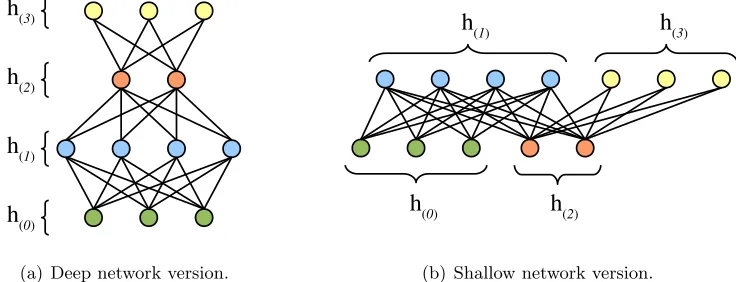
The derivations, proofs and algorithms given in this work for RBMs/BMs automatically extend to DBMs since each DBM can be transformed to an RBM with restricted connections and partially unknown input data. This is illustrated for a DBM with four layers in Figure 1. As a consequence of this relation DBMs can essentially be trained in the same way as RBMs but also suffer from the same problems as described before. The major difference in DBM
(a) Deep network version. (b) Shallow network version.
Figure 1: Example for (a) a DBM or an ANN with four layers h(0),· · · , h(3) and (b) the equivalent two layer shallow version of the same network with restricted connec-tions and unknown inputh(2).
How to Center Deep Boltzmann Machines
training compared to RBM training is that the expectation under the data distribution in the LL gradient of DBMs gets intractable. Due to the partially missing input data the factorization trick used for the calculation of expectation under the data distribution in RBMs cannot be applied anymore. Instead the term is approximated by running a mean field estimation until convergence (Salakhutdinov and Hinton, 2009), which corresponds to approximating the gradient of the variational lower bound of the LL. Furthermore, it is common to pre-train DBMs in a greedy layer wise fashion using RBMs (Salakhutdinov and Hinton, 2009; Hinton and Salakhutdinov, 2012).
4. Centering in Artificial Neural Networks in General
Removing the mean from visible and hidden units was originally proposed for feed forward neural networks (LeCun et al., 1998; Schraudolph, 1998). When this idea was applied to the visible units of RBMs (Tang and Sutskever, 2011) the model was reparameterized such that the probability distribution defined by the normal and centered RBM stayed the same. In this section we generalize this concept to show that centering is an alternative pa-rameterization for arbitrary ANN architectures in general, if the network is reparameterized accordingly. Consider the centered artificial neuron model
oj = φj X
i
wij(ai−µi) +cj !
, (16)
where the outputoj of the jth neuron depends on its activation function φj, bias term cj and weights wij with associated inputsai and their corresponding offsetsµi. Such neurons can be used to construct arbitrary network architectures using undirected, directed and recurrent connections, which can then be optimized with respect to a chosen loss.
Two different ANNs that represent exactly the same functional input-output mapping can be considered as different parameterizations of the same model. Thus, a centered ANN is just a different parameterization of an uncentered ANN if we can show that their functional input-output mappings are the same. This can be guaranteed in general if all corresponding units in a centered and an uncentered ANN have the same mapping from inputs to outputs. If the offset µi is changed to ˜µi = µi+∇µi then the output of the centered artificial neuron (16) becomes
φj X
i
wij(ai−µ˜i) +cj !
= φj X
i
wij(ai−(µi+∇µi)) +cj !
= φj X
i
wij(ai−µi) +cj− X
i
wij∇µi !
,
showing that the unit’s output does not change when changing the offset µi to ˜µi if the unit’s bias parameter cj is reparameterized to ˜cj =cj +Piwij∇µi. This generalizes the reparameterization for RBMs given by Equations (10) – (12) to ANNs. Now, by settingµi or ˜µi to zero it follows that for each normal ANN there exists a centered ANN and vice
versa such that the output of each neuron and thus the functional mapping from input to output of the whole network stays the same. This holds independently of the chosen
melchior, fischer and wiskott
activation functions, loss function and connection types including directed, undirected and recurrent connections.
Moreover, if we guarantee that a shift ofai implies a shift ofµi by the same value (that is, a shift ofai toai+δiimplies a shift ofµitoµi+δi) the neuron’s outputoj gets invariant to shifts of ai. This is easy to see since δi cancels out in Equation (16) if the same shift is applied to both ai and µi, which holds for example if we set the offsets to the mean values of the corresponding variables since hai+δii=haii+δi.
Note that, the original centering algorithm (LeCun et al., 1998; Schraudolph, 1998) did not reparameterize the network, which can cause instabilities especially if the learning rate is large.
4.1 Auto Encoders
An AE or auto-associator (Rumelhart et al., 1986b) is a type of ANN (and can thus be centered) that has originally been proposed for unsupervised dimensionality reduction. Like RBMs, AEs have also been used for unsupervised feature extraction and greedy layer-wise pre-training of deep neural networks (Bengio et al., 2007), and therefore fit well in this study for analyzing centering in ANNs.
In general, an AE consists of a deterministic encoderencode(x), which maps the input
x = (x1, ..., xN) to a hidden representation h = (h1, ..., hM) and a deterministic decoder
decode(h), which maps the hidden representation to the reconstructed input representation
˜
x. The network is optimized such that the reconstructed input ˜x gets as close as possible to the original input xmeasured by a chosen lossL(x,x˜). Common choices for the loss are the mean squared errorhPN
i=1(xi−x˜i)2idfor arbitrary input and the average cross entropy
h−PN
i=1xilog ˜xi+ (1−xi) log(1−x˜i)idfor binary data. AEs are usually trained via back-propagation (Kelley, 1960; Rumelhart et al., 1986a) and they can be seen as feed-forward neural networks where the input patterns are also the desired output patterns. We can therefore define a centered AE by centering the encoder and decoder, which for a centered three layer AE corresponds to
encode(x) = φenc W0(x−µ) +c = h,
decode(h) = φdec(W(h−λ) +b) = ˜x,
with encoder matrix W0, decoder matrix W, encoder bias c, decoder bias b, encoder offsetµ, decoder offsetλ, encoder activation functionφenc and decoder activation function
φdec. It is common to assume tied weights, which means that the encoder matrix is just the transpose of the decoder matrix (W0 = WT). Although this reduces the number of free parameters AEs can still learn trivial representations if the number of hidden units is not chosen to be much smaller than the number of input dimensions or if the network is not regularized. Common regularized variants of AEs are denoising AEs (Vincent et al., 2008), sparse AEs (Olshausen et al., 1996; Poultney et al., 2006; Ng, 2011) and contractive AEs (Bishop, 1995; Rifai et al., 2011).
When choosing the activation functions for the encoder and decoder (that are sigmoid, tangens-hyperbolicus, radial-basis, linear, linear-rectifier, ... ), we have to ensure that the encoder activation function is appropriate for the input data (for example a sigmoid cannot represent negative values). It is worth mentioning that when using the sigmoid function
How to Center Deep Boltzmann Machines
for φenc and φdec and tied weights, the encoder becomes equivalent to Equation (5) and the decoder becomes equivalent to Equation (6). The network structure therefore becomes equivalent to an RBM such that the only difference is the training objective (that is the loss function).
4.2 Initialization of the Model Parameters
It is a common way to initialize the weight matrix of ANNs to small random values to break the symmetry. The bias parameters are often initialized to zero. However, we argue that there exists a more reasonable initialization for the bias parameters.
Hinton (2010) has proposed to initialize the RBM’s visible bias parameterbito ln(pi/(1−
pi)), where pi is the proportion of the data points in which unitiis on (that ispi=hxiid). He has stated that if this is not done, the hidden units are used to activate the ith visible unit with a probability of approximately pi in the early stage of training.
We argue that this initialization is in fact reasonable since it corresponds to the Maxi-mum Likelihood Estimate (MLE) of the visible bias given the data for an RBM with zero weight matrix, given by
b∗= ln
hxid 1− hxid
=−ln
1
hxid −1
=σ−1(hxid) , (17)
where σ−1 is the inverse sigmoid function. Note that the MLE of the visible bias for an
RBM with zero weights is the same whether the RBM is centered or not. The conditional probability of the visible variables of an RBM with this initialization is then given by
p(x=1|h) = σ(σ−1(hxid)) = hxid, where p(x=1|h) denotes the vector containing the
elementsp(xi = 1|h). Thus, the mean of the data is initially modeled only by the bias values and the weights are free to model higher order statistics in the beginning of training. For the unknown hidden variables it is reasonable to assume an initial mean of 0.5 so that the MLE of the hidden bias for an RBM with zero weights is given by c∗ = σ−1(0.5) = 0.0. These considerations still hold approximately if the weights are not zero but initialized to small random values. For bigger initial weight values the model can be initially centered by using the inverse sigmoid of the average hidden activity given the data (c∗ =σ−1(hp(h=1|x)id))
for the hidden biases.
Montavon and M¨uller (2012) have suggested to initialize the bias parameters of centered DBMs to the inverse sigmoid of the initial offset parameters. They have argued that this initialization leads to a good starting point, because it guarantees that the Boltzmann machine is initially centered. Actually, if the initial offsets are set toµi=hxiidandλj = 0.5 the initialization suggested by Montavon and M¨uller (2012) is equal to the initialization to the MLEs as follows from Equation (17).
Note that this initialization is not restricted to RBMs or the sigmoid activation function. Independently of the initial weight matrix we can always set the bias in ANNs to the inverse activation function of the corresponding mean value.
5. Methods
As shown in Section 3 the algorithms described by Cho et al. (2011), Tang and Sutskever (2011) and Montavon and M¨uller (2012) can all be viewed as different ways of applying
melchior, fischer and wiskott
the centering trick. They differ in the choice of the offset parameters and in the way of approximating them, either based on the samples gained from the model in the previous learning step or from the current one, using an exponentially moving average or not. The question arises, how RBMs should be centered to achieve the best performance in terms of the LL. In Section 5 we therefore empirically analyze the different ways of centering and try to achieve a deeper understanding of why centering is beneficial.
For simplicity we introduce the following shorthand notation. The letter d denotes the data mean h·id, m denotes the model mean h·im, a denotes the average of the means
1
2h·id+ 12h·im, and 0 is used if the offsets are set to zero. We indicate the choice of µ in
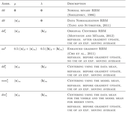
the first and the choice of λ in the second place, for example dm translates to µ = hxid and λ =hhim. We add a superscribedb (before) or l (later/after) to denote whether the reparameterization is performed before or after the gradient update. If the sliding factor in Algorithm 1 or 2 is set to a value smaller than one and thus an exponentially moving average is used, a subscript s (sliding) is added. Thus, we represent the variant of Cho
Abbr. µ λ Description
00 0 0 Normal binary RBM
(Smolensky, 1986)
d0 hxid 0 Data Normalization RBM
(Tang and Sutskever, 2011)
ddl
s hxid hhid Original Centered RBM
(Montavon and M¨uller, 2012) reparam. after gradient update, use of an exp. moving average
aab 0.5 (
hxid+hxim) 0.5 (hhid+hhim) Enhanced gradient RBM (Cho et al., 2011)
reparam. before gradient update, no use of an exp. moving average
ddb
s hxid hhid Centering using the data mean,
reparam. before gradient update, use of an exp. moving average
mmb
s hxim hhim Centering using the model mean,
reparam. before gradient update, use of an exp. moving average
dmb
s hxid hhim Centering using the data mean
for the visible and the model mean for hidden units,
reparam. before gradient update, use of an exp. moving average
Table 1: Look-up table: Abbreviations for the most frequently used algorithms.
How to Center Deep Boltzmann Machines
et al. (2011) byaab, the one of Montavon and M¨uller (2012) byddl
s, the data normalization of Tang and Sutskever (2011) by d0, and the normal binary RBM simply by 00. Table 1 summarizes the abbreviations most frequently used in this paper.
We begin our analysis with experiments on RBMs, where one layer is small enough to guarantee that the exact LL is still tractable. In a first set of experiments we analyze the four algorithms described above in terms of the evolution of the LL during training. In a second set of experiments we analyze the effect of the initializations described in Section 4.2. We proceed with a comparison of the effects of estimating offset values and reparameterizing the parameters before or after the gradient update. Afterwards we analyze the effects of using an exponentially moving average to approximate the offset values in the different algorithms and of choosing other offset values. We then compare the normal and the centered gradient with the natural gradient. Finally, to verify whether the results scale to more realistic problem sizes we compare RBMs, DBMs and AE on ten large data sets.
5.1 Benchmark Problems
We consider twelve different benchmark problems in our detailed analysis, see also Figure 2. TheBars & Stripes (MacKay, 2003) data set consists of patterns of sizeD×Dthat can be generated as follows. First, for each row of a pattern all corresponding pixels are either set to zero or to one with equal probability. Second, with a probability of 0.5 the pattern is rotated by 90 degrees. This leads to N = 2D+1 patterns where the completely uniform patterns occur twice as often as the others. The data set is symmetric in terms of the amount of zeros and ones and thus the flipped and unflipped problems are equivalent. An upper bound of the LL is given by (N −4) ln N1+ 4 ln N2. For our experiments we used
D = 3 or D = 2 (only in Section 6.9) leading to an upper bound of −41.59 and −13.86, respectively.
The Shifting Bar data set is an artificial benchmark problem we have designed to be asymmetric in terms of the amount of zeros and ones in the data. The data set consists of vectors of sizeN where a set ofB successive pixels with cyclic boundary conditions are set to one, the ’bar’, and the others are set to zero. More formally the data set can be generated as follows, beginning with a vector where all pixels are set to zero, an index 0≤i < N is chosen uniformly at random. The pixel with index iand the followingB−1 pixels, which underly cyclic boundary conditions are set to one (that is the pixels with indices{i, (i+ 1) mod N , . . . ,(i+B−1) modN} are set to one). This leads toN different patterns with equal probability, and an upper bound of the LL of Nln N1, the percentage of ones in the data set is NB. For our experiments we used N = 9, B = 1 and its flipped version Flipped Shifting Bar, which we get forN = 9, B = 8, both having an upper LL bound of −19.78.
TheMNIST (LeCun et al., 1998) data set of handwritten digits has become a standard benchmark problem for RBMs. It consists of 60,000 training and 10,000 testing examples of gray value handwritten digits of size 28×28. Usually, in a first preprocessing step the values are normalized to lie in [0,1]. Across different studies the normalized values are then either used directly as input, or the data set is binarized using a threshold of 0.5 or by sampling according to the normalized values that are treated as probabilities.4 In this study
4. In Appendix D we give a an comparison of normal and centered RBMs on the differentMNISTversions.
melchior, fischer and wiskott
(a) 8 out of 16 patterns from theBars & Stripes data set.
(b) All patterns of theShifting Bar data set withN = 9 andB= 1.
(c) Example patterns from theMNIST data set after binarization.
(d) Example patterns from theCaltech 101 Silhouette data set.
Figure 2: Some patterns from the different benchmark problems.
we binarizedMNIST with a threshold of 0.5. The data set contains 13.3% ones, similar to theShifting Bar problem, which for our choice ofN and B contains 11.1% ones. We refer to the data set where each bit ofMNIST is flipped (that is each one is replaced by a zero and vice versa) as 1-MNIST.
The CalTech 101 Silhouettes (Marlin et al., 2010) data set consists of 4100 training, 2307 validation, and 2264 testing examples of binary object silhouettes of size 28×28. The data set contains 55.1% ones, and thus (like in theBars & Stripes problem) the amount of zeros and ones is almost the same. The background pixels take the value one, which is in contrast toMNIST where the background pixels are set to zero.
In some experiments we also considered the eightUCI binary (Larochelle et al., 2010; Larochelle and Murray, 2011) data sets from different domains comprising biological, im-age, text and game-related data. The data sets differ in dimensionality (112 to 500) and size (a few hundred to several thousand examples) and have been separated into training, validation, and test sets. All UCI binary data sets contain less ones than zeros, where the percentage of ones lies between 3.9% and 36.8%.
How to Center Deep Boltzmann Machines
6. Results
For all models in this work the weight matrices were initialized with random values sampled from a Gaussian with zero mean and a standard deviation of 0.01. If not stated otherwise the visible biases, hidden biases, and offsets were initialized as described in Section 4.2.
We began our analysis with experiments on small RBMs where the LL can be calculated exactly, where we used 4 hidden units when modelingBars & Stripes andShifting Bar and 16 hidden units when modelingMNIST. For training we used CD-1, PCD-1 and PTc(with
c = 10 or c = 20) where the c temperatures were distributed uniformly from 0 to 1. For
Bars & Stripes and Shifting Bar full-batch training was performed for 50,000 gradient updates, where the LL was evaluated every 50th gradient update. For modeling MNIST
mini-batch training with a batch size of 100 was performed for 100 epochs, each consisting of 600 gradient updates and the exact LL was evaluated after each epoch. Note that in order to get an unbiased comparison of the different models, we did not use any additional modifications of the update rule like a momentum term, weight decay or an annealing learning rate.
The tables in this work show the maximum average LL and the corresponding standard deviation reached during training averaged over 25 trials. In addition the final average LL reached at the end of training is given in parenthesis to indicate a potential divergence of the LL. For some computational expensive experiments we used only 10 trials, which will be mentioned explicitly. For reasons of readability, the LL values for the big data sets were normalized to the number of training samples. In order to check if the result of the best method within one row differs significantly from the others we performed pairwise signed Wilcoxon rank-sum tests (with p = 0.05). The best results are highlighted in bold. This can be more than one value if the significance test between these values was negative.
6.1 Comparison of the Standard Methods
The comparison of the learning performance of the previously described algorithmsddl
s,aab,
d0, and 00 (using their originally proposed initializations) shows that training a centered RBM leads to significantly higher LL values than training a normal binary RBM (see Table 2 for the results on Bars & Stripes and MNIST and Table 3 for the results on Shifting Bar
and Flipped Shifting Bar).
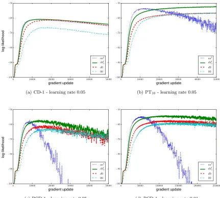
Figure 3 illustrates on the Bars & Stripes data set that centering (aab, ddl
s, and d0) leads to faster learning and higher LL values than normal RBMs (00). This differs from the observations made for DBMs by Montavon and M¨uller (2012), who have found a better generative performance of centering only in the case of locally connected DBMs. Further-more, Figure 3 shows that centering both the visible and the hidden variables (ddl
sandaab)
compared to centering only the visible variables (d0) accelerates learning and leads to a higher LL. This is different from the observations made for RBMs by Tang and Sutskever (2011), who have stated that centering only the visible variables leads to a performance similar to that of the enhanced gradient. Thus centered RBMs where visible and hidden variables are centered can form more accurate models of the data distribution than normal RBMs and centered RBMs where only the visible variables are centered.
It can also be seen from Figure 3 that all methods show divergence in combination with CD and PCD (as described before by Fischer and Igel, 2010, for normal RBMs), which
melchior, fischer and wiskott
is prevented for ddl
s, d0, and 00 when using PT as shown in Figure 3(b). This can be explained by the fact that PT leads to faster mixing Markov chains and thus less biased gradient approximations. The aa algorithm however suffers from severe divergence of the LL when PCD or PT is used, which is even worse than with CD. This divergence problem does occur independently of the choice of the learning rate as indicated by the LL values reached at the end of training (given in parentheses) in Table 2 and Table 3, and which can
0 10000 20000 30000 40000 50000
gradient update −100 −90 −80 −70 −60 −50 lo g-lik el ih oo d aab ddl s d0 00
(a) CD-1 - learning rate 0.05
0 10000 20000 30000 40000 50000
gradient update −100 −90 −80 −70 −60 −50 lo g-lik el ih oo d aab ddl s d0 00
(b) PT10 - learning rate 0.05
0 10000 20000 30000 40000 50000
gradient update −100 −90 −80 −70 −60 −50 lo g-lik el ih oo d aab ddl s d0 00
(c) PCD-1 - learning rate 0.05
0 50000 100000 150000 200000 250000 gradient update −100 −90 −80 −70 −60 −50 lo g-lik el ih oo d aab ddl s d0 00
(d) PCD-1 - learning rate 0.01
Figure 3: Evolution of the average LL on the training data for models with 4 hidden units on the Bars & Stripes data set for the standard centering methods. (a) CD-1 with a learning rate of η = 0.05, (b) PT10 with a learning rate of η = 0.05, (c)
PCD-1 with a learning rate of η = 0.05, and (d) PCD-1 with a learning rate of
η= 0.01.
Ho
w
to
Center
Deep
Bol
tzmann
Ma
chines
Algorithm-η aab ddls d0 00
Bars & Stripes
CD-1-0.1 -61.66 ±1.71 (-69.1) -61.33 ±1.89 (-69.1) -61.73 ±4.19 (-70.9) -66.53 ±3.47 (-78.1) CD-1-0.05 -61.09 ±1.89 (-65.0) -60.82 ±2.31 (-64.2) -61.23 ±3.70 (-65.1) -66.35 ±4.24 (-71.2) CD-1-0.01 -61.08 ±1.60 (-61.1) -61.31 ±1.55 (-61.3) -63.30 ±3.02 (-63.3) -68.56 ±2.94 (-68.6) PCD-1-0.1 -59.05 ±2.07 (-360.6) -58.93 ±2.24 (-102.7) -62.46 ±4.65 (-97.3) -63.28 ±5.61 (-84.3) PCD-1-0.05 -57.25 ±1.51 (-167.4) -57.01 ±1.61 (-65.4) -60.42 ±5.19 (-72.5) -62.29 ±4.84 (-70.6) PCD-1-0.01 -54.86 ±0.98 (-55.3) -56.80 ±0.73 (-56.8) -61.03 ±3.74 (-61.0) -64.61 ±2.95 (-64.6) PT10-0.1 -54.67 ±3.43 (-202.5) -51.99 ±1.13 (-52.2) -56.18 ±5.32 (-56.7) -54.89 ±3.66 (-55.3) PT10-0.05 -53.34 ±0.99 (-70.7) -52.21 ±1.06 (-52.5) -56.54 ±5.82 (-56.6) -56.46 ±4.43 (-56.8) PT10-0.01 -53.63 ±1.25 (-53.8) -56.76 ±0.79 (-56.8) -61.26 ±4.58 (-61.3) -64.71 ±3.52 (-64.7) MNIST
CD-1-0.1 -153.01 ±2.32 (-158.0) -153.46 ±2.45 (-155.5) -153.89 ±2.91 (-155.0) -170.29 ±2.45 (-170.6) CD-1-0.05 -153.07 ±1.51 (-156.0) -152.78 ±3.57 (-153.8) -153.01 ±2.80 (-155.4) -169.43 ±2.95 (-169.7) CD-1-0.01 -152.90 ±1.38 (-152.9) -152.42 ±2.15 (-152.4) -153.77 ±2.54 (-153.8) -172.70 ±1.86 (-172.8) PCD-1-0.1 -150.78 ±1.95 (-174.9) -144.10 ±1.67 (-144.7) -154.64 ±3.14 (-156.6) -183.11 ±8.62 (-183.2) PCD-1-0.05 -146.83 ±1.54 (-163.4) -141.93 ±1.25 (-142.9) -146.86 ±2.08 (-147.5) -185.78 ±6.78 (-185.8) PCD-1-0.01 -143.36 ±0.74 (-144.1) -140.43 ±0.62 (-140.7) -141.88 ±1.02 (-141.9) -193.60 ±4.56 (-193.6) PT10-0.01 -259.50 ±17.54 (<-999) -142.00 ±1.04 (-142.3) -145.84 ±2.49 (-147.4) -152.38 ±3.05 (-152.4)
Table 2: Maximum average LL on the training data for centered and normal RBMs (top) with 4 hidden units on the Bars & Stripes data set and (bottom) with 16 hidden units on the MNIST data set using different sampling methods and learning ratesη. Each LL value is followed by the corresponding standard deviation of the 25 trials and the average LL at the end of training is given in parenthesis.
melchior,
fischer
and
wisk
ott
Algorithm-η aab ddls d0 00
Shifting Bar
CD-1-0.2 -21.04 ±1.41 (-21.9) -20.42 ±0.85 (-20.4) -22.15 ±1.38 (-22.5) -22.32 ±1.46 (-22.6) CD-1-0.1 -21.29 ±1.18 (-21.5) -20.76 ±0.80 (-20.8) -21.35 ±0.95 (-21.4) -21.56 ±0.94 (-21.6) CD-1-0.05 -21.16 ±0.84 (-21.2) -22.74 ±0.65 (-22.7) -26.89 ±0.29 (-26.9) -26.11 ±0.40 (-26.1) PCD-1-0.2 -23.07 ±0.78 (-237.2) -22.48 ±0.85 (-33.6) -23.15 ±1.01 (-31.9) -23.34 ±0.75 (-31.7) PCD-1-0.1 -22.14 ±0.70 (-87.4) -21.92 ±0.66 (-24.0) -22.75 ±0.84 (-23.7) -22.64 ±1.15 (-23.3) PCD-1-0.05 -21.71 ±0.73 (-26.0) -22.53 ±0.55 (-22.5) -26.84 ±0.36 (-26.8) -26.06 ±0.48 (-26.1) PT10-0.2 -21.30 ±0.81 (-31.9) -20.66 ±0.67 (-20.8) -21.47 ±1.13 (-21.6) -22.12 ±1.17 (-22.3) PT10-0.1 -20.84 ±0.62 (-21.5) -20.57 ±0.56 (-20.6) -21.34 ±0.90 (-21.4) -21.21 ±0.93 (-21.2) PT10-0.05 -20.78 ±0.88 (-20.8) -22.42 ±0.69 (-22.4) -26.96 ±0.30 (-27.0) -26.18 ±0.38 (-26.2)
Flipped Shifting Bar
CD-1-0.2 -20.82 ±1.15 (-21.3) -20.73 ±1.06 (-20.8) -22.04 ±1.62 (-22.3) -28.14 ±0.27 (-28.2) CD-1-0.1 -20.85 ±1.05 (-20.9) -20.90 ±0.83 (-20.9) -21.17 ±0.84 (-21.2) -28.35 ±0.04 (-28.4) CD-1-0.05 -21.18 ±0.82 (-21.2) -22.64 ±0.65 (-22.6) -26.85 ±0.34 (-26.9) -28.31 ±0.02 (-28.3) PCD-1-0.2 -22.73 ±0.88 (-310.8) -22.35 ±0.91 (-29.1) -23.48 ±0.84 (-32.6) -28.19 ±0.28 (-28.3) PCD-1-0.1 -22.15 ±0.71 (-88.3) -21.64 ±0.72 (-22.6) -22.38 ±0.88 (-23.2) -28.35 ±0.04 (-28.4) PCD-1-0.05 -21.72 ±0.86 (-25.6) -22.34 ±0.60 (-22.3) -26.90 ±0.34 (-26.9) -28.31 ±0.02 (-28.3) PT10-0.2 -21.13 ±0.72 (-32.4) -20.57 ±0.63 (-20.6) -21.14 ±0.84 (-21.4) -28.17 ±0.26 (-28.2) PT10-0.1 -21.03 ±0.81 (-21.6) -20.73 ±0.74 (-20.8) -21.26 ±0.72 (-21.3) -28.35 ±0.04 (-28.4) PT10-0.05 -21.01 ±0.86 (-21.1) -22.48 ±0.73 (-22.5) -26.87 ±0.35 (-26.9) -28.31 ±0.02 (-28.3)
Table 3: Maximum average LL on the training data for centered and normal RBMs with 4 hidden units on (top) theShifting Bar
data set and (bottom) the Flipped Shifting Bar data set using different sampling methods and learning rates η. Each LL value is followed by the corresponding standard deviation of the 25 trials and the average LL at the end of training is given in parenthesis.
How to Center Deep Boltzmann Machines
also be seen by comparing Figure 3(c) and Figure 3(d). The divergence occurs earlier and is more severe for bigger learning rates, while for the other algorithms we never observed divergence in combination with PT even for very big learning rates and long training time. The reasons for this divergence are discussed in detail in Section 6.4.
The results in Table 3 also demonstrate the flip invariance of the centered RBMs on the
Shifting Bar data set empirically. Whereas00 fails to model the flipped version of the data set correctly,ddl
s,aab, andd0 have approximately the same performance on the flipped and unflipped data set.
6.2 Initialization
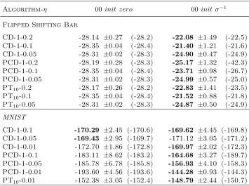
The experiments in this section were done to analyze the effects of different initializations of the parameters as discussed in Section 4.2. First, we trained normal binary RBMs (that is 00) where the visible bias was initialized to zero or to the inverse sigmoid of the data mean. In both cases the hidden bias was initialized to zero. Table 4 shows the results for normal binary RBMs trained on the Flipped Shifting Bar data set, where RBMs with zero initialization failed to learn the distribution accurately. The RBMs using the inverse sigmoid initialization achieved better performance and therefore seem to be less sensitive
Algorithm-η 00 init zero 00init σ−1
Flipped Shifting Bar
CD-1-0.2 -28.14 ±0.27 (-28.2) -22.08 ±1.49 (-22.5) CD-1-0.1 -28.35 ±0.04 (-28.4) -21.40 ±1.21 (-21.6) CD-1-0.05 -28.31 ±0.02 (-28.3) -24.90 ±0.47 (-24.9) PCD-1-0.2 -28.19 ±0.28 (-28.3) -25.17 ±1.32 (-42.3) PCD-1-0.1 -28.35 ±0.04 (-28.4) -23.71 ±0.98 (-26.7) PCD-1-0.05 -28.31 ±0.02 (-28.3) -24.99 ±0.57 (-25.0) PT10-0.2 -28.17 ±0.26 (-28.2) -22.83 ±1.41 (-23.5) PT10-0.1 -28.35 ±0.04 (-28.4) -21.52 ±0.88 (-21.8) PT10-0.05 -28.31 ±0.02 (-28.3) -24.87 ±0.50 (-24.9) MNIST
CD-1-0.1 -170.29 ±2.45 (-170.6) -169.62 ±4.45 (-169.8) CD-1-0.05 -169.43 ±2.95 (-169.7) -171.12 ±3.05 (-171.2) CD-1-0.01 -172.70 ±1.86 (-172.8) -169.97 ±2.02 (-172.3) PCD-1-0.1 -183.11 ±8.62 (-183.2) -164.68 ±3.27 (-189.7) PCD-1-0.05 -185.78 ±6.78 (-185.8) -156.93 ±4.10 (-158.3) PCD-1-0.01 -193.60 ±4.56 (-193.6) -144.28 ±0.93 (-144.3) PT10-0.01 -152.38 ±3.05 (-152.4) -148.79 ±2.44 (-150.7)
Table 4: Maximum average LL on the training data for normal RBMs (top) with 4 hidden units on theFlipped Shifting Bar data set and (bottom) with 16 hidden units on theMNIST data set, where the visible bias is initialized to zero or to the inverse sigmoid of the data mean.
melchior, fischer and wiskott
Algorithm-η ddls init zero ddls init σ−1
Flipped Shifting Bar
CD-1-0.2 -20.76 ±0.95 (-20.8) -20.73 ±1.06 (-20.8) CD-1-0.1 -20.82 ±0.88 (-20.8) -20.90 ±0.83 (-20.9) CD-1-0.05 -22.98 ±0.73 (-23.0) -22.64 ±0.65 (-22.6) PCD-1-0.2 -22.32 ±0.82 (-31.8) -22.35 ±0.91 (-29.1) PCD-1-0.1 -21.75 ±0.60 (-22.6) -21.64 ±0.72 (-22.6) PCD-1-0.05 -22.79 ±0.64 (-22.8) -22.34 ±0.60 (-22.3) PT10-0.2 -20.37 ±0.36 (-20.6) -20.57 ±0.63 (-20.6) PT10-0.1 -20.74 ±0.75 (-20.8) -20.73 ±0.74 (-20.8) PT10-0.05 -22.95 ±0.70 (-22.9) -22.48 ±0.73 (-22.5)
Table 5: Maximum average LL on the training data for centered RBMs (ddl
s) with 4 hidden units on the Flipped Shifting Bar data set, where the visible bias is initialized to zero or to the inverse sigmoid of the data mean.
to the ‘difficulty’ of the data representation. However, the results are not as good as the results of the centered RBMs shown in Table 3. The same observations can be made when training RBMs on the MNIST data set (see Table 4 bottom). The RBMs with inverse sigmoid initialization achieved significantly better results than RBMs initialized to zero in the case of PCD and PT, but still worse compared to the centered RBMs. Furthermore, using the inverse sigmoid initialization allows us to achieve similar performance onMNIST
and 1-MNIST, while the RBM with zero initialization failed to learn the distribution for
1-MNIST at all (results not shown). A visual comparison of the filters of normal RBMs trained on MNIST and 1-MNIST has already been given by Cho et al. (2011) and Tang and Sutskever (2011).
We then trained models using the centering versions dd, aa, and d0 comparing the initialization suggested in Section 4.2 against the initialization to zero. In most cases the results showed no significant difference in terms of the maximum LL reached in trials with different initializations, or slightly better results were found when using the inverse sigmoid in combination with a small learning rate. This can be explained by the better starting point yielded by this initialization. See Table 5 for the results forddl
s on theFlipped Shifting Bar data set as an example. We therefore used the inverse sigmoid initialization in the following experiments since it was beneficial for normal RBMs.
6.3 Reparameterization
To investigate the effects of performing the reparameterization before or after the gradient update during training of centered RBMs , we analyzed the learning behavior of ddb
s (the
algorithm suggested here) andddl
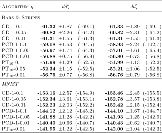
s(the algorithm suggested by Montavon and M¨uller, 2012) on all data sets. The results for RBMs trained on the Bars & Stripes data set and the
MNIST data set are given in Table 6 (top). No significant difference between the two versions can be observed and the same result (not shown) was obtained for theShifting Bar
How to Center Deep Boltzmann Machines
Algorithm-η ddbs ddls
Bars & Stripes
CD-1-0.1 -61.32 ±1.87 (-69.1) -61.33 ±1.89 (-69.1) CD-1-0.05 -60.82 ±2.26 (-64.2) -60.82 ±2.31 (-64.2) CD-1-0.01 -61.31 ±1.55 (-61.3) -61.31 ±1.55 (-61.3) PCD-1-0.1 -59.08 ±1.53 (-94.5) -58.93 ±2.24 (-102.7) PCD-1-0.05 -56.97 ±1.74 (-64.3) -57.01 ±1.61 (-65.4) PCD-1-0.01 -56.88 ±0.75 (-56.9) -56.80 ±0.73 (-56.8) PT10-0.1 -51.99 ±1.29 (-52.5) -51.99 ±1.13 (-52.2) PT10-0.05 -52.34 ±1.15 (-52.5) -52.21 ±1.06 (-52.5) PT10-0.01 -56.76 ±0.77 (-56.8) -56.76 ±0.79 (-56.8) MNIST
CD-1-0.1 -153.16 ±2.57 (-154.9) -153.46 ±2.45 (-155.5) CD-1-0.05 -152.34 ±3.61 (-153.1) -152.78 ±3.57 (-153.8) CD-1-0.01 -152.23 ±2.03 (-152.2) -152.42 ±2.15 (-152.4) PCD-1-0.1 -144.12 ±2.12 (-145.2) -144.10 ±1.67 (-144.7) PCD-1-0.05 -141.88 ±1.28 (-142.2) -141.93 ±1.25 (-142.9) PCD-1-0.01 -140.40 ±0.66 (-140.7) -140.43 ±0.62 (-140.7) PT10-0.01 -141.95 ±1.22 (-142.5) -142.00 ±1.04 (-142.3)
Table 6: Maximum average LL on the training data for RBMs (top) with 4 hidden units on theBars & Stripes data set and (bottom) with 16 hidden units on theMNIST
data set, using the reparameterization before (ddb
s) and after (ddls) the gradient update.
and the Flipped Shifting Bar data set. We therefore reparameterize the RBMs before the gradient update in the remainder of this work. This is also motivated by the fact that the enhanced gradient is only equivalent to centering using the average of model and data mean for visible and hidden offsets if the model is reparameterized before it is updated (that is, the enhanced gradient is equivalent toaab but not toaal).
6.4 Analyzing the Model-Mean-Related Divergence Effect
The severe divergence problem observed when using the enhanced gradient in combination with PCD or PT raises the question whether the problem is induced by setting the offsets to 0.5(hxid+hxim) and 0.5(hhid+hhim) or by bad sampling based estimates of gradient and offsets. We therefore trained centered RBMs with 9 visible and 4 hidden units on the
Bars & Stripes data set using either the exact gradient where only hxim and hhim were approximated by samples or using PT10estimates of the gradient whilehximandhhim were
calculated exactly. Figure 4(a) shows that if the exact gradient is used but the offsets are estimated, no divergence foraain combination with PT is observed and the performance of
aa and dd become almost equivalent. Interestingly, the divergence is also prevented if the gradient is estimated using PT but the offsets are calculated exactly as shown in Figure 4(b).
melchior, fischer and wiskott
0 10000 20000 30000 40000 50000
gradient update
−100 −90 −80 −70 −60 −50
lo
g-lik
el
ih
oo
d
aab
ddb
d0 00
(a) Exact gradient with approximated offsets
0 10000 20000 30000 40000 50000
gradient update
−100 −90 −80 −70 −60 −50
lo
g-lik
el
ih
oo
d
aab(exact means)
(b) PT10with exact means
Figure 4: Evolution of the average LL on the training data for RBMs with 4 hidden units on the Bars & Stripes data set for the standard centering methods. (a) When the exact gradient is used but the offsets are estimated using PT10and (b) when
PT10is used for estimating the gradient but the offsets are calculated exactly. In
both cases the learning rate wasη = 0.05.
Thus, the divergence behavior must be induced by approximating both, gradient and offsets. The fact that the mean under the data distribution can always be calculated exactly might explain why we do not observe divergence for ddin combination with PT.
To further deepen the understanding of the divergence effect we investigated the param-eter evolution during training of RBMs with different offsets. We observed that the change of the offset values between two gradient updates gets extremely large during training when using the model mean. Figure 5(a) shows in an exemplary manner the evolution of the first hidden offset λ1 for a single trial, where the approximated offset forddb is almost constant
while it is rather large for aab and even bigger for mmb (the centering variant that uses the mean of hidden and visible variables under the model distribution as offsets). In each iteration we calculated the exact offsets to estimate the approximation error shown in Fig-ure 5(b). Obviously, there is no approximation error for dd while the error for aa quickly gets large and the error for mm gets even twice as big. In combination with the gradient approximation error this causes the weight matrices foraa and mmto grow extremely big as shown in Figure 5(c). Consistent with the even larger approximation error for the offset estimate ofmm, the divergence formm becomes even worse than that foraa, as shown in Figure 6.
To further confirm that the divergence is not just caused by the additional sampling noise introduced by approximating the offsets, we trained a centered RBM using PT for the gradient approximation while we set the offsets to uniform random values between zero and one in each iteration. The results are shown in Figure 6(a) and demonstrate that even random offset values do not lead to the divergence problems. Thus, the divergence cannot
How to Center Deep Boltzmann Machines
be caused by additional sampling noise but rather by the correlated errors of gradient and offset approximations. To test this hypothesis we investigated mmb where the samples for offset and gradient approximations were taken from different PT sampling processes. The results are shown in Figure 6(b) where no divergence can be observed anymore. While creating two sets of samples for gradient and offset approximations prevents the LL from diverging it almost doubles the computational cost and can therefore not be considered as a reasonable solution in practice. Moreover, using the model mean as offset still leads to
10000 10100 10200 10300 10400 10500
gradient update 0.0
0.2 0.4 0.6 0.8 1.0
λ1
aab
ddb
mmb
(a) Close up of the offset evolution forλ1
0 10000 20000 30000 40000 50000 gradient update
0.0 0.2 0.4 0.6 0.8 1.0
A ve ra ge hi dd en of fs et ap pr ox im at io n er ro
r aab
ddb
mmb
(b) Evolution of the offset approximation error
0 10000 20000 30000 40000 50000 gradient update 0 100 200 300 400 500 600 Fr ob en iu s no rm of th e w ei gh tm at rix aab ddb mmb
(c) Evolution of the weight norm
Figure 5: Evolution of the offsets and weights of different centered variants for RBMs with 4 hidden units during training on Bars & Stripes using PT10. For clearness a
single trial is shown, but the experiments were repeated 25 times and all trials showed qualitatively the same results. (a) Close up of the evolution of offsetλ1
over 500 gradient updates. (b) The evolution of the absolute difference between exact and approximated hidden offset averaged over all hidden units. (c) The evolution of the Frobenius norm of the weight matrices.
melchior, fischer and wiskott
0 10000 20000 30000 40000 50000
gradient update
−34 −32 −30 −28 −26 −24 −22 −20
lo
g-lik
el
ih
oo
d
aab
ddb
mmb
00
(Random means)b
(a) Random offsets
0 20000 40000 60000 80000 100000 gradient update
−34 −32 −30 −28 −26 −24 −22 −20
lo
g-lik
el
ih
oo
d
aab
ddb
mmb
(b) Independent approximations
Figure 6: Evolution of the average LL on the training data for RBMs with 4 hidden units on the Shifting Bars data set using PT10 with a learning rate of η = 0.1. (a)
Normal RBMs, centered RBMs, and centered RBMs with random offset values (denoted by Random meansb). (b) Centered RBMs when the samples for the offset approximations come from a different Markov chain than the samples used for the gradient approximation.
slightly worse final LL values than using the mean under the data distribution. This might be explained by the fact that the additional approximation of the model mean introduces noise while the data mean can be estimated exactly. Note, that the divergence also occurs if either only visible or hidden offsets are set to the PT-approximated model mean, which can be seen for example fordmin Figure 7(b).
Interestingly, the observed initially faster learning speed of mm and aa, which can be seen in Figure 6(a), does not occur anymore when offset and gradient approximation are based on different sample sets. This observation can also be made when the exact gradient is used (see Figure 4a). Thus, the initially faster learning speed seems also be caused by the correlated approximations of gradient and offsets and could be explained by the rapidly growing norm of the weight matrix shown in Figure 5(c), which effectively leads to a bigger step size in the parameter updates.
Note, that divergence can either be caused by using the expectation under the model distribution for the offset approximations as described in this section or by the bias of the gradient approximation introduced by using only a few steps of Gibbs sampling (Fischer and Igel, 2010; Schulz et al., 2010; Fischer and Igel, 2011). The latter can occur for all methods when CD or PCD is used for training. Furthermore, the LL can also decrease on the test data due to overfitting to the training data, which is not divergence in the proper sense.