Robust Kernel Density Estimation
JooSeuk Kim [email protected]
Clayton D. Scott∗ [email protected]
Electrical Engineering and Computer Science University of Michigan
Ann Arbor, MI 48109-2122 USA
Editor: Kenji Fukumizu
Abstract
We propose a method for nonparametric density estimation that exhibits robustness to contamina-tion of the training sample. This method achieves robustness by combining a tradicontamina-tional kernel density estimator (KDE) with ideas from classical M-estimation. We interpret the KDE based on a positive semi-definite kernel as a sample mean in the associated reproducing kernel Hilbert space. Since the sample mean is sensitive to outliers, we estimate it robustly via M-estimation, yielding a robust kernel density estimator (RKDE).
An RKDE can be computed efficiently via a kernelized iteratively re-weighted least squares (IRWLS) algorithm. Necessary and sufficient conditions are given for kernelized IRWLS to con-verge to the global minimizer of the M-estimator objective function. The robustness of the RKDE is demonstrated with a representer theorem, the influence function, and experimental results for density estimation and anomaly detection.
Keywords: outlier, reproducing kernel Hilbert space, kernel trick, influence function, M-estimation
1. Introduction
The kernel density estimator (KDE) is a well-known nonparametric estimator of univariate or multi-variate densities, and numerous articles have been written on its properties, applications, and exten-sions (Silverman, 1986; Scott, 1992). However, relatively little work has been done to understand or improve the KDE in situations where the training sample is contaminated. This paper addresses a method of nonparametric density estimation that generalizes the KDE, and exhibits robustness to contamination of the training sample.1
Consider training data following a contamination model
X1, . . . ,Xn iid
∼(1−p)f0+p f1,
where f0is the “nominal” density to be estimated, f1is the density of the contaminating distribution, and p< 12 is the proportion of contamination. Labels are not available, so that the problem is unsupervised. The objective is to estimate f0 while making no parametric assumptions about the nominal or contaminating distributions.
∗. Also in the Department of Statistics.
Clearly f0 cannot be recovered if there are no assumptions on f0,f1 and p. Instead, we will focus on a set of nonparametric conditions that are reasonable in many practical applications. In particular, we will assume that, relative to the nominal data, the contaminated data are
(a) outlying: the densities f0and f1have relatively little overlap (b) diffuse: f1is not too spatially concentrated relative to f0 (c) not abundant: a minority of the data come from f1
Although we will not be stating these conditions more precisely, they capture the intuition behind the quantitative results presented below.
As a motivating application, consider anomaly detection in a computer network. Imagine that several multi-dimensional measurements X1, . . . ,Xnare collected. For example, each Ximay record
the volume of traffic along certain links in the network, at a certain instant in time (Chhabra et al., 2008). If each measurement is collected when the network is in a nominal state, these data could be used to construct an anomaly detector by first estimating the density f0 of nominal measurements, and then thresholding that estimate at some level to obtain decision regions. Unfortunately, it is often difficult to know that the data are free of anomalies, because assigning labels (nominal vs. anomalous) can be a tedious, labor intensive task. Hence, it is necessary to estimate the nominal density (or a level set thereof) from contaminated data. Furthermore, the distributions of both nom-inal and anomalous measurements are potentially complex, and it is therefore desirable to avoid parametric models.
The proposed method achieves robustness by combining a traditional kernel density estimator with ideas from M-estimation (Huber, 1964; Hampel, 1974). The KDE based on a translation invari-ant, positive semi-definite (PSD) kernel is interpreted as a sample mean in the reproducing kernel Hilbert space (RKHS) associated with the kernel. Since the sample mean is sensitive to outliers, we estimate it robustly via M-estimation, yielding a robust kernel density estimator (RKDE). We de-scribe a kernelized iteratively re-weighted least squares (KIRWLS) algorithm to efficiently compute the RKDE, and provide necessary and sufficient conditions for the convergence of KIRWLS to the RKDE.
We also offer three arguments to support the claim that the RKDE robustly estimates the nominal density and its level sets. First, we characterize the RKDE by a representer theorem. This theorem shows that the RKDE is a weighted KDE, and the weights are smaller for more outlying data points. Second, we study the influence function of the RKDE, and show through an exact formula and numerical results that the RKDE is less sensitive to contamination by outliers than the KDE. Third, we conduct experiments on several benchmark data sets that demonstrate the improved performance of the RKDE, relative to competing methods, at both density estimation and anomaly detection.
Density estimation with positive semi-definite kernels has been studied by several authors. Vap-nik and Mukherjee (2000) optimize a criterion based on the empirical cumulative distribution func-tion over the class of weighted KDEs based on a PSD kernel. Shawe-Taylor and Dolia (2007) provide a refined theoretical treatment of this approach. Song et al. (2008) adopt a different cri-terion based on Hilbert space embeddings of probability distributions. Our approach is somewhat similar in that we attempt to match the mean of the empirical distribution in the RKHS, but our criterion is different. These methods were also not designed with contaminated data in mind.
We show that the standard kernel density estimator can be viewed as the solution to a certain least squares problem in the RKHS. The use of quadratic criteria in density estimation has also been previously developed. The aforementioned work of Song et al. optimizes the norm-squared in Hilbert space, whereas Kim (1995), Girolami and He (2003), Kim and Scott (2010) and Ma-hapatruni and Gray (2011) adopt the integrated squared error. Once again, these methods are not designed for contaminated data.
Previous work combining robust estimation and kernel methods has focused primarily on su-pervised learning problems. M-estimation applied to kernel regression has been studied by various authors (Christmann and Steinwart, 2007; Debruyne et al., 2008a,b; Zhu et al., 2008; Wibowo, 2009; Brabanter et al., 2009). Robust surrogate losses for kernel-based classifiers have also been studied (Xu et al., 2006). In unsupervised learning, a robust way of doing kernel principal com-ponent analysis, called spherical KPCA, has been proposed, which applies PCA to feature vectors projected onto a unit sphere around the spatial median in a kernel feature space (Debruyne et al., 2010). The kernelized spatial depth was also proposed to estimate depth contours nonparametrically (Chen et al., 2009). To our knowledge, the RKDE is the first application of M-estimation ideas in kernel density estimation.
In Section 2 we propose robust kernel density estimation. In Section 3 we present a representer theorem for the RKDE. In Section 4 we describe the KIRWLS algorithm and its convergence. The influence function is developed in Section 5, Section 6 describes a straightforward extension to non-reproducing kernels, and experimental results are reported in Section 7. Conclusions are offered in Section 8. Section 9 contains proofs of theorems. Matlab code implementing our algorithm is available atwww.eecs.umich.edu/˜cscott.
2. Robust Kernel Density Estimation
Let X1, . . . ,Xn∈Rd be a random sample from a distribution F with a density f . The kernel density
estimate of f , also called the Parzen window estimate, is a nonparametric estimate given by
b
fKDE(x) =
1 n
n
∑
i=1kσ(x,Xi)
where kσ is a kernel function with bandwidthσ. To ensure that bfKDE(x) is a density, we assume
the kernel function satisfies kσ(·,·)≥0 andRkσ(x,·)dx=1. We will also assume that kσ(x,x′)
is translation invariant, in that kσ(x−z,x′−z) =kσ(x,x′)for all x,x′, and z.
In addition, we require that kσ be positive semi-definite, which means that the matrix
(kσ(xi,xj))1≤i,j≤mis positive semi-definite for all positive integers m and all x1, . . . ,xm∈Rd.
Well-known examples of kernels satisfying all of the above properties are the Gaussian kernel
kσ(x,x′) =
1
√
2πσ d
exp
−kx−x′k
2 2σ2
the multivariate Student kernel
kσ(x,x′) =
1
√πσ
d
·Γ (ν+d)/2
Γ(ν/2) ·
1+1
ν·k
x−x′k2
σ2
−ν+d
2 ,
and the Laplacian kernel
kσ(x,x′) = cd
σdexp
−kx−σx′k
where cd is a constant depending on the dimension d that ensuresRkσ(x,·)dx=1 (Scovel et al.,
2010).
Every PSD kernel kσis associated with a unique Hilbert space of functions called its reproducing kernel Hilbert space (RKHS) which we will denote
H
, and kσ is called the reproducing kernel ofH
. For every x,Φ(x),kσ(·,x)is an element ofH
, and therefore so too is the KDE. See Steinwart and Christmann (2008) for a thorough treatment of PSD kernels and RKHSs. For our purposes, the critical property ofH
is the so-called reproducing property. It states that for all g∈H
and allx∈Rd, g(x) =hΦ(x),giH. As a special case, taking g=kσ(·,x′), we obtain
kσ(x,x′) =hΦ(x),Φ(x′)iH
for all x,x′ ∈Rd. We also note that, by translation invariance, the functions Φ(x) have constant norm in
H
becausekΦ(x)k2
H =hΦ(x),Φ(x)iH =kσ(x,x) =kσ(0,0).
We will denoteτ=kΦ(x)kH.
From this point of view, the KDE can be expressed as
b
fKDE(·) =
1 n
n
∑
i=1kσ(·,Xi)
=1
n
n
∑
i=1Φ(Xi),
the sample mean of theΦ(Xi)’s in
H
. Equivalently, fbKDE∈H
is the solution ofmin
g∈H
n
∑
i=1kΦ(Xi)−gk2H.
Being the solution of a least squares problem, the KDE is sensitive to the presence of outliers among theΦ(Xi)’s. To reduce the effect of outliers, we propose to use M-estimation (Huber, 1964)
to find a robust sample mean of theΦ(Xi)’s. For a robust loss functionρ(x)on x≥0, the robust
kernel density estimate is defined as
b
fRKDE=arg min g∈H
n
∑
i=1ρ kΦ(Xi)−gkH
. (2)
Well-known examples of robust loss functions are Huber’s or Hampel’sρ. Unlike the quadratic loss, these loss functions have the property thatψ,ρ′is bounded. Huber’sρandψare given by
ρ(x) =
(
ψ(x) =
(
x ,0≤x≤a
a ,a<x, (3)
and Hampel’sρandψare
ρ(x) =
x2/2 ,0≤x<a
ax−a2/2 ,a≤x<b a(x−c)2/2(b−c) +a(b+c−a)/2 ,b≤x<c a(b+c−a)/2 ,c≤x
ψ(x) =
x ,0≤x<a a ,a≤x<b a·(c−x)/(c−b) ,b≤x<c
0 ,c≤x.
(4)
The functionsρ(x),ψ(x), andψ(x)/x are plotted in Figure 1, for the quadratic, Huber, and Hampel losses. Note that while ψ(x)/x is constant for the quadratic loss, for Huber’s or Hampel’s loss, this function is decreasing in x. This is a desirable property for a robust loss function, which will be explained later in detail. While our examples and experiments employ Huber’s and Hampel’s losses, many other losses can be employed.
We will argue below that bfRKDEis a valid density, having the form∑ni=1wikσ(·,Xi)with weights
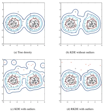
wi that are nonnegative and sum to one. To illustrate the estimator, Figure 2 (a) shows a contour
plot of a Gaussian mixture distribution onR2. Figure 2 (b) depicts a contour plot of a KDE based on a training sample of size 200 from the Gaussian mixture. As we can see in Figure 2 (c) and (d), when 20 contaminating data points are added, the KDE is significantly altered in low density regions, while the RKDE is much less affected.
We remark that the definition of the RKDE does not require that kσ be a reproducing kernel, only that the functionsΦ(x) =kσ(·,x)belong to a Hilbert space. Indeed, almost all of the results presented below hold in this more general setting. However, we restrict our attention to reproducing kernels for two reasons. First, with reproducing kernels, inner products in
H
can be easily computed via the kernel, leading to efficient implementation. Second, the reproducing property allows us to interpret the representer theorem and influence function to infer robustness of the RKDE. With non-reproducing kernels, these interpretations are less clear. The extension to non-RKHS Hilbert spaces is discussed in Section 6, with specific examples.Throughout this paper, we defineϕ(x),ψ(x)/x and consider the following assumptions onρ,
ψ, andϕ:
(A1) ρis non-decreasing,ρ(0) =0, andρ(x)/x→0 as x→0
(A2) ϕ(0),limx→0ψ(xx) exists and is finite (A3) ψandϕare continuous
(A4) ψandϕare bounded
(A5) ϕis Lipschitz continuous
x
ρ
(x
)
Quadratic Huber Hampel
(a)ρfunctions
x
ψ
(x
)
Quadratic Huber Hampel
(b)ψfunctions
x
ψ
(x
)/
x
Quadratic Huber Hampel
(c)ψ(x)/x
Figure 1: The comparison between three differentρ(x),ψ(x), andψ(x)/x: quadratic, Huber’s, and Hampel’s.
3. Representer Theorem
In this section, we will describe how bfRKDE can be expressed as a weighted combination of the
kσ(·,Xi)’s. A formula for the weights explains how a robust sample mean in
H
translates to arobust nonparametric density estimate. We also present necessary and sufficient conditions for a function to be an RKDE. From (2), bfRKDE =arg ming∈HJ(g), where
J(g) =1
n
n
∑
i=1−6 −4 −2 0 2 4 6 −6
−4 −2 0 2 4 6
(a) True density
−6 −4 −2 0 2 4 6 −6
−4 −2 0 2 4 6
(b) KDE without outliers
−6 −4 −2 0 2 4 6 −6
−4 −2 0 2 4 6
(c) KDE with outliers
−6 −4 −2 0 2 4 6 −6
−4 −2 0 2 4 6
(d) RKDE with outliers
Figure 2: Contours of a nominal density (a) and kernel density estimates (b-d) along with data samples from the nominal density (o) and contaminating density (x). 200 points are from the nominal distribution and 20 contaminating points are from a uniform distribution.
First, let us find necessary conditions for g to be a minimizer of J. Since the space over which we are optimizing J is a Hilbert space, the necessary conditions are characterized through Gateaux differentials of J. Given a vector space
X
and a function T :X
→R, the Gateaux differential of T at x∈X
with incremental h∈X
is defined asδT(x; h) =lim
α→0
T(x+αh)−T(x)
IfδT(x0; h) is defined for all h∈
X
, a necessary condition for T to have a minimum at x0 is that δT(x0; h) =0 for all h∈X
(Luenberger, 1997). From this optimality principle, we can establish the following lemma.Lemma 1 Suppose assumptions (A1) and (A2) are satisfied. Then the Gateaux differential of J at g∈
H
with incremental h∈H
isδJ(g; h) =−V(g),hH
where V :
H
→H
is given byV(g) =1
n
n
∑
i=1ϕ(kΦ(Xi)−gkH)· Φ(Xi)−g
.
A necessary condition for g=fbRKDE is V(g) =0.
Lemma 1 is used to establish the following representer theorem, so named because bfRKDE can
be represented as a weighted combination of kernels centered at the data points. Similar results are known for supervised kernel methods (Sch¨olkopf et al., 2001).
Theorem 2 Suppose assumptions (A1) and (A2) are satisfied. Then, b
fRKDE(x) = n
∑
i=1wikσ(x,Xi) (6)
where wi≥0,∑ni=1wi=1. Furthermore,
wi∝ ϕ(kΦ(Xi)−bfRKDEkH). (7)
It follows that bfRKDEis a density. The representer theorem also gives the following interpretation
of the RKDE. Ifϕis decreasing, as is the case for a robust loss, then wiwill be small whenkΦ(Xi)−
b
fRKDEkH is large. Now for any g∈
H
,kΦ(Xi)−gk2H =hΦ(Xi)−g,Φ(Xi)−giH
=kΦ(Xi)k2H −2hΦ(Xi),giH +kgk2H
=τ2−2g(X
i) +kgk2H,
where the last step follows from the reproducing property. Taking g=bfRKDE, we see that wiis small
when bfRKDE(Xi)is small. Therefore, the RKDE is robust in the sense that it down-weights outlying
points.
Theorem 2 provides a necessary condition for bfRKDE to be the minimizer of (5). With an
addi-tional assumption on J, this condition is also sufficient.
Theorem 3 Suppose that assumptions (A1) and (A2) are satisfied, and J is strictly convex. Then (6), (7), and∑ni=1wi=1 are sufficient for bfRKDE to be the minimizer of (5).
Lemma 4 J is strictly convex provided either of the following conditions is satisfied: (i) ρis strictly convex and non-decreasing.
(ii) ρis convex, strictly increasing, n≥3, and K= (kσ(Xi,Xj))ni,j=1is positive definite.
The second condition implies that J can be strictly convex even for the Huber loss, which is convex but not strictly convex.
4. KIRWLS Algorithm and Its Convergence
In general, (2) does not have a closed form solution and bfRKDE has to be found by an iterative
algorithm. Fortunately, the iteratively re-weighted least squares (IRWLS) algorithm used in classical M-estimation (Huber, 1964) can be extended to a RKHS using the kernel trick. The kernelized iteratively re-weighted least squares (KIRWLS) algorithm starts with initial w(i0)∈R, i=1, . . . ,n such that wi(0)≥0 and∑ni=1wi(0)=1, and generates a sequence{f(k)}by iterating on the following procedure:
f(k)= n
∑
i=1w(ik−1)Φ(Xi),
w(ik)= ϕ(kΦ(Xi)−f
(k)k
H)
∑n
j=1ϕ(kΦ(Xj)−f(k)kH)
.
Intuitively, this procedure is seeking a fixed point of Equations (6) and (7). The computation of
kΦ(Xj)−f(k)kH can be done by observing
kΦ(Xj)−f(k)k2H =
D
Φ(Xj)−f(k),Φ(Xj)−f(k)
E
H
=Φ(Xj),Φ(Xj)
H −2
Φ
(Xj),f(k)
H +
f(k),f(k)H.
Since f(k)=∑ni=1wi(k−1)Φ(Xi), we have
Φ
(Xj),Φ(Xj)
H = kσ(Xj,Xj)
Φ
(Xj),f(k)
H =
n
∑
i=1w(ik−1)kσ(Xj,Xi)
f(k),f(k)H = n
∑
i=1n
∑
l=1wi(k−1)wl(k−1)kσ(Xi,Xl).
Recalling thatΦ(x) =kσ(·,x), after the kth iteration
f(k)(x) = n
∑
i=1w(ik−1)kσ(x,Xi).
KIRWLS can also be viewed as a kind of optimization transfer/majorize-minimize algorithm (Lange et al., 2000; Jacobson and Fessler, 2007) with a quadratic surrogate forρ. This perspective is used in our analysis in Section 9.4, where f(k)is seen to be the solution of a weighted least squares problem in
H
.The next theorem characterizes the convergence of KIRWLS in terms of {J(f(k))}∞k=1 and
{f(k)}∞k=1.
Theorem 5 Suppose assumptions (A1) - (A3) are satisfied, andϕ(x)is nonincreasing. Let
S
=g∈H
V(g) =0and{f(k)}∞k=1 be the sequence produced by the KIRWLS algorithm. Then, J(f(k))monotonically decreases at every iteration and converges. Also,
S
6=/0andkf(k)−
S
kH ,infg∈Skf
(k)−gk
H →0
as k→∞.
In words, as the number of iterations grows, f(k) becomes arbitrarily close to the set of stationary points of J, points g∈
H
satisfyingδJ(g; h) =0 ∀h∈H
.Corollary 6 Suppose that the assumptions in Theorem 5 hold and J is strictly convex. Then{f(k)}∞k=1 converges to bfRKDE in the
H
-norm and the supremum norm.Proof Convergence in the
H
-norm follows from the previous result because under strict convexity of J,|S
|=1. Convergence in the supremum norm now follows from the reproducing property and Cauchy-Schwarz because, for any x,|f(k)(x)−bfRKDE(x)|=|hΦ(x),f(k)−bfRKDEiH|
≤τkf(k)−fbRKDEkH.
5. Influence Function for Robust KDE
To quantify the robustness of the RKDE, we study the influence function. First, we recall the traditional influence function from robust statistics. Let T(F)be an estimator of a scalar parameter based on a distribution F. As a measure of robustness of T , the influence function was proposed by Hampel (1974). The influence function (IF) for T at F is defined as
IF(x′; T,F) =lim
s→0
T((1−s)F+sδx′)−T(F)
s ,
where δx′ represents a discrete distribution that assigns probability 1 to the point x′. Basically,
For example, the maximum likelihood estimator for the unknown mean of a Gaussian distribu-tion is the sample mean T(F),
T(F) =EF[X] =
Z
x dF(x). (8)
The influence function for T(F)in (8) is
IF(x′; T,F) =lim
s→0
T((1−s)F+sδx′)−T(F)
s
=x′−EF[X].
Since|IF(x′; T,F)|increases without bound as x′ goes to±∞, the estimator is considered to be not robust.
Now, consider a similar concept for a function estimate. Since the estimate is a function, not a scalar, we should be able to express the change of the function value at every x.
Definition 7 (IF for function estimate) Let T(x; F)be a function estimate based on F, evaluated at x. We define the influence function for T(x; F)as
IF(x,x′; T,F) =lim
s→0
T(x; Fs)−T(x; F)
s
where Fs= (1−s)F+sδx′.
IF(x,x′; T,F) represents the change of the estimated function T at x when we add infinitesimal probability mass at x′to F. For example, the standard KDE is
T(x; F) = bfKDE(x; F) =
Z
kσ(x,y)dF(y) =EF[kσ(x,X)]
where X∼F. In this case, the influence function is
IF(x,x′;fbKDE,F) =lim s→0
b
fKDE(x; Fs)−bfKDE(x; F)
s
=lim
s→0
EFs[kσ(x,X)]−EF[kσ(x,X)]
s
=lim
s→0
−sEF[kσ(x,X)] +sEδx′[kσ(x,X)]
s
=−EF[kσ(x,X)] +Eδx′[kσ(x,X)]
=−EF[kσ(x,X)] +kσ(x,x′). (9)
With the empirical distribution Fn=1n∑ni=1δXi,
IF(x,x′;bfKDE,Fn) =−
1 n
n
∑
i=1kσ(x,Xi) +kσ(x,x′). (10)
To investigate the influence function of the RKDE, we generalize its definition to a general distribution µ, writing fbRKDE(·; µ) = fµwhere
fµ=arg min g∈H
Z
For the robust KDE, T(x,F) = bfRKDE(x; F) =hΦ(x),fFiH, we have the following characterization
of the influence function. Let q(x) =xψ′(x)−ψ(x).
Theorem 8 Suppose assumptions (A1)-(A5) are satisfied. In addition, assume that fFs → fF as
s→0. If ˙fF ,lims→0 fFs−sfF exists, then
IF(x,x′;bfRKDE,F) = f˙F(x)
where ˙fF ∈
H
satisfiesZ
ϕ(kΦ(x)−fFkH)dF
·f˙F
+
Z f˙
F,Φ(x)−fF
H
kΦ(x)−fFk3H
·q(kΦ(x)−fFkH)· Φ(x)−fF
dF(x)
= (Φ(x′)−fF)·ϕ(kΦ(x′)−fFkH). (11)
Unfortunately, for Huber or Hampel’sρ, there is no closed form solution for ˙fF of (11).
How-ever, if we work with Fninstead of F, we can find ˙fFn explicitly. Let
1= [1, . . . ,1]T,
k′= [kσ(x′,X1), . . . ,kσ(x′,Xn)]T,
Inbe the n×n identity matrix, K,(kσ(Xi,Xj))ni=1,j=1be the kernel matrix, Q be a diagonal matrix with Qii=q(kΦ(Xi)−fFnkH)/kΦ(Xi)−fFnk
3
H,
γ= n
∑
i=1ϕ(kΦ(Xi)−fFnkH),
and
w= [w1, . . . ,wn]T,
where w gives the RKDE weights as in (6).
Theorem 9 Suppose assumptions (A1)-(A5) are satisfied. In addition, assume that
• fFn,s → fFn as s→0 (satisfied when J is strictly convex)
• the extended kernel matrix K′based on{Xi}ni=1 S
{x′}is positive definite. Then,
IF(x,x′;bfRKDE,Fn) = n
∑
i=1αikσ(x,Xi) +α′kσ(x,x′)
where
α′=n·ϕ(kΦ(x′)−f
FnkH)/γ
andα= [α1, . . . ,αn]T is the solution of the following system of linear equations:
γIn+ (In−1·wT)TQ(In−1·wT)K
α
= −nϕ(kΦ(x′)−fFnkH)w−α′(In−1·w
T)TQ
−5 0 5 10 15 true
KDE RKDE(Huber) RKDE(Hampel)
(a)
−5 0 5 10 15
KDE RKDE(Huber) RKDE(Hampel) outlier
(b)
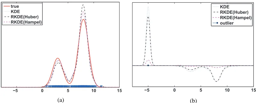
Figure 3: (a) true density and density estimates. (b) IF as a function of x when x′=−5
Note that α′ captures the amount by which the density estimator changes near x′ in response to contamination at x′. Nowα′is given by
α′= ϕ(kΦ(x′)−fFnkH)
1
n∑ n
i=1ϕ(kΦ(Xi)−fFnkH)
.
For a standard KDE, we haveϕ≡1 andα′=1, in agreement with (10). For robustρ,ϕ(kΦ(x′)−
fFnkH)can be viewed as a measure of “inlyingness”, with more inlying points having larger values.
This follows from the discussion just after Theorem 2, which leverages the reproducing property. If the contaminating point x′is less inlying than the average Xi, thenα′<1. Thus, the RKDE is less
sensitive to outlying points than the KDE.
As mentioned above, in classical robust statistics, the robustness of an estimator can be inferred from the boundedness of the corresponding influence function. However, the influence functions for density estimators are bounded even ifkx′k →∞. Therefore, when we compare the robustness of density estimates, we compare how close the influence functions are to the zero function.
Simulation results are shown in Figure 3 for a synthetic univariate distribution. Figure 3 (a) shows the density of the distribution, and three estimates. Figure 3 (b) shows the corresponding influence functions. As we can see in (b), for a point x′in the tails of F, the influence functions for the robust KDEs are overall smaller, in absolute value, than those of the standard KDE (especially with Hampel’s loss). Additional numerical results are given in Section 7.2.
Finally, it is interesting to note that for any density estimator f ,b Z
IF(x,x′;bf,F)dx=lim
s→0 R b
f(x; Fs)dx−
R b
f(x; F)dx
s =0.
Thusα′=−∑n
i=1αi for a robust KDE. This suggests that since fbRKDE has a smaller increase at x′
(compared to the KDE), it will also have a smaller decrease (in absolute value) near the training data. Therefore, the norm of IF(x,x′;bfRKDE,Fn), viewed as a function of x, should be smaller when
6. Generalization to Other Hilbert Spaces
So far, we have focused our attention on PSD kernels and viewed the KDE as an element of the RKHS associated with the kernel. However, the RKDE can be defined in a more general setting. In particular, it is only necessary that the functionsΦ(x) =kσ(·,x)belong to a Hilbert space
H
. Then one can still obtain all the previous results, that is, Lemmas 1 and 4, Theorems 2, 3, 5, 8, and 9, and Corollary 6 (except convergence in the supremum norm). (For Theorems 8 and 9 it is necessary to additionally assume thatkΦ(x)kH is bounded independent of x.) The only necessary change isthat inner products of the formhΦ(x),Φ(x′)iH can no longer be computed as kσ(x,x′). Thus, K in
Lemma 4 (ii), k′,K,K′ in Theorem 9, and various terms in the KIRWLS algorithm should now be computed with the inner product on
H
.It is also interesting to note that this generalization gives a representer theorem for non-RKHS Hilbert spaces. This contrasts with standard approaches to supervised learning that minimize an empirical risk plus regularization term. In those cases, a representer theorem may be more difficult to obtain when the function class is not an RKHS.
There are some examples of non-RKHS Hilbert spaces where the inner product can still be computed efficiently. For example, consider
H
=L2(Rd)and denote˜kσ(x,x′) =hΦ(x),Φ(x′)iL2(Rd) =
Z
kσ(z,x)kσ(z,x′)dz. For the multivariate Gaussian kernel, ˜kσ=k√
2σ. For the multivariate Cauchy kernel (the multivari-ate Student kernel withν=1; see Section 2), it holds that ˜kσ(x,x′) =k2σ(x,x′)(Berry et al., 1996). For the multivariate Laplacian product kernel,
kσ(x,x′) = 1 (2σ)dexp
−kx−σx′k1
,
it is true that
˜kσ(x,x′) = 1 (4σ)d
d
∏
l=1
1+|xl−x′l|
σ
exp
−kx−σx′k1
.
For kernels without a closed-form expression for ˜kσ, the inner product may still be calculated nu-merically. For radially symmetric kernels this entails a simple one-dimensional table, as ˜kσ(x,x′)
depends only onkx−x′k, and these values may be tabulated in advance.
As we noted previously, however, we rely on the reproducing property to deduce robustness of the RKDE from the representer theorem and the influence function. For non-RKHS Hilbert spaces, these arguments are less clear. We have not experimentally investigated non-reproducing kernels, and so cannot comment on the robustness of RKDEs based on such kernels in practice.
7. Experiments
The experimental setup is described in 7.1, and results are presented in 7.2.
7.1 Experimental Setup
7.1.1 DATA
We conduct experiments on 15 benchmark data sets (Banana, B. Cancer, Diabetes, F. Solar, Ger-man, Heart, Image, Ringnorm, Splice, Thyroid, Twonorm, Waveform, Pima Indian, Iris, MNIST), which were originally used in the task of classification. The data sets are available online: see http://www.fml.tuebingen.mpg.de/Members/ for the first 12 data sets and the UCI machine learning repository for the last 3 data sets. There are 100 randomly permuted partitions of each data set into “training” and “test” sets (20 for Image, Splice, and MNIST).
Given X1, . . . ,Xn∼ f = (1−p)·f0+p·f1, our goal is to estimate f0, or the level sets of f0. For each data set with two classes, we take one class as the nominal data from f0 and the other class as contamination from f1. For Iris, there are 3 classes and we take one class as nominal data and the other two as contamination. For MNIST, we choose to use digit 0 as nominal and digit 1 as contamination. For MNIST, the original dimension 784 is reduced to 8 via kernel PCA using a Gaussian kernel with bandwidth 30. For each data set, the training sample consists of n0nominal data and n1contaminating points, where n1=ε·n0forε=0, 0.05, 0.10, 0.15, 0.20, 0.25 and 0.30. Note that eachεcorresponds to an anomaly proportion p such that p=1+εε. n0is always taken to be the full amount of training data for the nominal class.
7.1.2 METHODS
In our experiments, we compare three density estimators: the standard kernel density estimator (KDE), variable kernel density estimator (VKDE), and robust kernel density estimator (RKDE) with Hampel’s loss. For all methods, the Gaussian kernel in (1) is used as the kernel function kσand the kernel bandwidthσis set as the median distance of a training point Xito its nearest neighbor.
The VKDE has a variable bandwidth for each data point,
b
fV KDE(x) =
1 n
n
∑
i=1kσi(x,Xi),
and the bandwidthσiis set as
σi=σ·
η
b fKDE(Xi)
1/2
whereηis the mean of{bfKDE(Xi)}ni=1(Abramson, 1982; Comaniciu et al., 2001). There is another implementation of the VKDE whereσiis based on the distance to its k-th nearest neighbor (Breiman
et al., 1977). However, this version did not perform as well and is therefore omitted.
For the RKDE, the parameters a, b, and c in (4) are set as follows. First, we compute bfmed,
which is the RKDE obtained withρ=| · |, and set di=kΦ(Xi)−bfmedkH. Then, a is set to be the
median of{di}, b the 75th percentile of{di}, and c the 85th percentile of{di}. After finding these
parameters, we initialize w(i0)such that f(1)= bfmedand terminate KIRWLS when |J(f(k+1))−J(f(k))|
J(f(k)) <10− 8.
7.1.3 EVALUATION
at the tasks of density estimation and anomaly detection, respectively. In each case, an appropriate performance measure is adopted. These are explained in detail in Section 7.2. To compare a pair of methods across multiple data sets, we adopt the Wilcoxon signed-rank test (Wilcoxon, 1945). Given a performance measure, and given a pair of methods andε, we compute the difference hibetween
the performance of two density estimators on the ith data set. The data sets are ranked 1 through 15 according to their absolute values|hi|, with the largest|hi|corresponding to the rank of 15. Let R1 be the sum of ranks over these data sets where method 1 beats method 2, and let R2be the sum of the ranks for the other data sets. The signed-rank test statistic T ,min(R1,R2)and the corresponding p-value are used to test whether the performances of the two methods are significantly different. For example, the critical value of T for the signed rank test is 25 at a significance level of 0.05. Thus, if T ≤25, the two methods are significantly different at the given significance level, and the larger of R1and R2determines the method with better performance.
7.2 Experimental Results
We begin by studying influence functions.
7.2.1 SENSITIVITY USING INFLUENCE FUNCTION
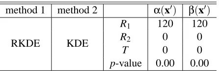
As the first measure of robustness, we compare the influence functions for KDEs and RKDEs, given in (10) and Theorem 9, respectively. To our knowledge, there is no formula for the influence function of VKDEs, and therefore VKDEs are excluded in the comparison. We examineα(x′) =
IF(x′,x′; T,Fn)and
β(x′) =
Z
IF(x,x′; T,Fn)
2 dx
1/2 .
In words,α(x′)reflects the change of the density estimate value at an added point x′andβ(x′)is an overall impact of x′on the density estimate overRd.
In this experiment,εis equal to 0, that is, the density estimators are learned from a pure nominal sample. Then, we take contaminating points from the test sample, each of which serves as an x′. This gives us multipleα(x′)’s andβ(x′)’s. The performance measures are the medians of{α(x′)}
and{β(x′)}(smaller means better performance). The results using signed rank statistics are shown in Table 1. The results clearly states that for all data sets, RKDEs are less affected by outliers than KDEs.
7.2.2 KULLBACK-LEIBLER(KL)DIVERGENCE
Second, we present the Kullback-Leibler (KL) divergence between density estimates bf and f0, DKL(bf||f0) =
Z b
f(x)log bf(x) f0(x)
dx.
This KL divergence is large whenever f estimates fb 0to have mass where it does not. For contami-nation characterized by properties (a), (b), and (c) in the Introduction, we expect this performance measure to capture the robustness of a density estimator.
The computation of DKLis done as follows. Since we do not know the nominal f0, it is estimated
method 1 method 2 α(x′) β(x′)
RKDE KDE
R1 120 120
R2 0 0
T 0 0
p-value 0.00 0.00
Table 1: The signed-rank statistics and p-values of the Wilcoxon signed-rank test using the medians of{α(x′)}and{β(x′)} as a performance measure. If R1 is larger than R2, method 1 is better than method 2.
data set. Then, the integral is approximated by the sample mean, that is,
DKL(bf||f0)≈ 1 n′
n′
∑
i=1log bf(x
′ i)
e f0(x′i)
where{x′i}ni=′1is an i.i.d sample from the estimated density f with nb ′=2n=2(n0+n1). Note that the estimated KL divergence can have an infinite value when ef0(y) =0 (to machine precision) and
b
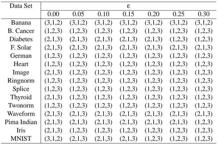
f(y)>0 for some y∈Rd. The averaged KL divergence over the permutations are used as the performance measure (smaller means better performance). In Table 2, the rank of the three methods are shown for each data set andε.
Table 3 summarizes the results using the Wilcoxon signed-rank test. When comparing RKDEs and KDEs, the results show that KDEs have smaller KL divergence than RKDEs withε=0. Asε increases, however, RKDEs estimate f0 more accurately than KDEs. The results also demonstrate that VKDEs are the worst in the sense of KL divergence. Note that VKDEs place a total mass of 1/n at all Xi, whereas the RKDE will place a mass wi<1/n at outlying points.
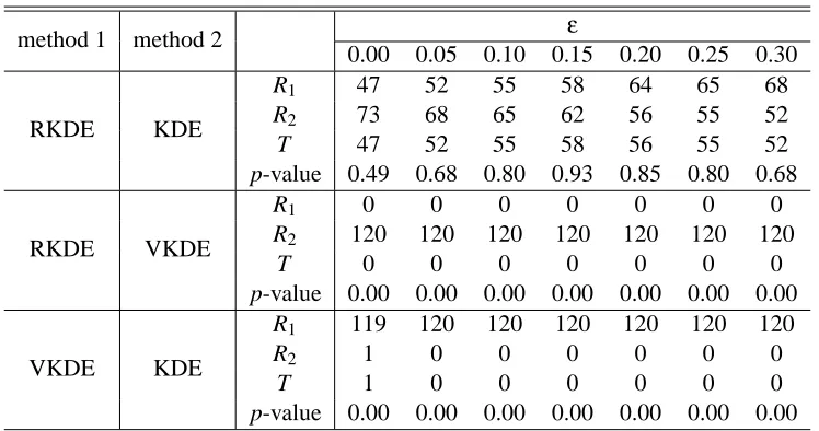
Since KL divergence is not symmetric, we also compute KL divergence between f0and bf ,
DKL(f0||bf) = Z
f0(x)log f0(x)
b f(x)dx =
Z
f0(x)log f0(x)dx− Z
f0(x)logbf(x)dx
This KL divergence is large whenever bf estimates f0not to have mass where it does.
Since f0is the same when comparing different estimate f , we only have to compare the secondb term, which is approximated as
−
Z
f0(x)logbf(x)dx≈ − 1 n′′
n′′
∑
i=1logbf(x′′i),
where{x′′i}ni=′′1 is a separate nominal sample, obtained from the test data. Table 4 and 5 show that with this KL divergence as performance measure, VKDE performs best for almost all data sets and
Data Set ε
0.00 0.05 0.10 0.15 0.20 0.25 0.30 Banana (3,1,2) (3,1,2) (3,1,2) (3,1,2) (3,1,2) (3,1,2) (3,1,2) B. Cancer (1,2,3) (1,2,3) (1,2,3) (1,2,3) (1,2,3) (1,2,3) (1,2,3) Diabetes (2,1,3) (2,1,3) (2,1,3) (2,1,3) (2,1,3) (1,2,3) (1,2,3) F. Solar (2,1,3) (2,1,3) (2,1,3) (2,1,3) (2,1,3) (2,1,3) (2,1,3) German (1,2,3) (1,2,3) (1,2,3) (1,2,3) (1,2,3) (1,2,3) (1,2,3) Heart (1,2,3) (1,2,3) (1,2,3) (1,2,3) (1,2,3) (1,2,3) (1,2,3) Image (2,1,3) (1,2,3) (1,2,3) (1,2,3) (1,2,3) (1,2,3) (1,2,3) Ringnorm (1,2,3) (1,2,3) (1,2,3) (1,2,3) (1,2,3) (1,2,3) (1,2,3) Splice (1,2,3) (1,2,3) (1,2,3) (1,2,3) (1,2,3) (1,2,3) (1,2,3) Thyroid (2,1,3) (1,2,3) (1,2,3) (1,2,3) (1,2,3) (1,2,3) (1,2,3) Twonorm (1,2,3) (1,2,3) (1,2,3) (1,2,3) (1,2,3) (1,2,3) (1,2,3) Waveform (2,1,3) (2,1,3) (2,1,3) (2,1,3) (2,1,3) (2,1,3) (2,1,3) Pima Indian (2,1,3) (2,1,3) (2,1,3) (2,1,3) (2,1,3) (2,1,3) (1,2,3) Iris (2,1,3) (1,2,3) (1,2,3) (1,2,3) (1,2,3) (1,2,3) (1,2,3) MNIST (3,1,2) (2,1,3) (2,1,3) (2,1,3) (1,2,3) (1,2,3) (1,2,3)
Table 2: The ranks of (RKDE, KDE, VKDE) using DKL(fb||f0) as a performance measure. For example, (2, 1, 3) means that KDE performs best, RKDE next, and VKDE worst.
7.2.3 ANOMALYDETECTION
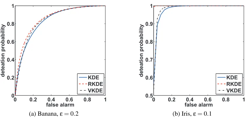
In this experiment, we apply the density estimators in anomaly detection problems. If we had a pure sample from f0, we would estimate f0and use{x :bf0(x)>λ}as a detector. For eachλ, we could get a false negative and false positive probability using test data. By varyingλ, we would then obtain a receiver operating characteristic (ROC) and area under the curve (AUC). However, since we have a contaminated sample, we have to estimate f0robustly. Robustness can be checked by comparing the AUC of the anomaly detectors, where the density estimates are based on the contaminated training data (higher AUC means better performance).
Examples of the ROCs are shown in Figure 4. The RKDE provides better detection probabilities, especially at low false alarm rates. This results in higher AUC. For each pair of methods and each
method 1 method 2 ε
0.00 0.05 0.10 0.15 0.20 0.25 0.30
RKDE KDE
R1 26 67 78 83 94 101 103
R2 94 53 42 37 26 19 17
T 26 53 42 37 26 19 17
p-value 0.06 0.72 0.33 0.21 0.06 0.02 0.01
RKDE VKDE
R1 104 117 117 117 117 119 119
R2 16 3 3 3 3 1 1
T 16 3 3 3 3 1 1
p-value 0.01 0.00 0.00 0.00 0.00 0.00 0.00
VKDE KDE
R1 0 0 0 0 0 0 0
R2 120 120 120 120 120 120 120
T 0 0 0 0 0 0 0
p-value 0.00 0.00 0.00 0.00 0.00 0.00 0.00
Table 3: The signed-rank statistics and p-values of the Wilcoxon signed-rank test using DKL(bf||f0) as a performance measure. If R1is larger than R2, method 1 is better than method 2.
0 0.2 0.4 0.6 0.8 1
0 0.2 0.4 0.6 0.8 1
false alarm
d
e
te
a
ti
o
n
p
ro
b
a
b
il
ity
KDE RKDE VKDE
(a) Banana,ε=0.2
0 0.2 0.4 0.6 0.8 1
0.5 0.6 0.7 0.8 0.9 1
false alarm
d
e
te
a
ti
o
n
p
ro
b
a
b
il
ity
KDE RKDE VKDE
(b) Iris,ε=0.1
Figure 4: Examples of ROCs.
8. Conclusions
Data Set ε
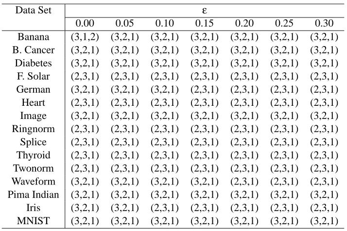
0.00 0.05 0.10 0.15 0.20 0.25 0.30 Banana (3,1,2) (3,2,1) (3,2,1) (3,2,1) (3,2,1) (3,2,1) (3,2,1) B. Cancer (3,2,1) (3,2,1) (3,2,1) (3,2,1) (3,2,1) (3,2,1) (3,2,1) Diabetes (3,2,1) (3,2,1) (3,2,1) (3,2,1) (3,2,1) (3,2,1) (3,2,1) F. Solar (2,3,1) (2,3,1) (2,3,1) (2,3,1) (2,3,1) (2,3,1) (2,3,1) German (3,2,1) (3,2,1) (3,2,1) (2,3,1) (2,3,1) (2,3,1) (2,3,1) Heart (2,3,1) (2,3,1) (2,3,1) (2,3,1) (2,3,1) (2,3,1) (2,3,1) Image (3,2,1) (3,2,1) (3,2,1) (3,2,1) (3,2,1) (3,2,1) (3,2,1) Ringnorm (2,3,1) (2,3,1) (2,3,1) (2,3,1) (2,3,1) (2,3,1) (2,3,1) Splice (2,3,1) (2,3,1) (2,3,1) (2,3,1) (2,3,1) (2,3,1) (2,3,1) Thyroid (2,3,1) (2,3,1) (2,3,1) (2,3,1) (2,3,1) (2,3,1) (2,3,1) Twonorm (2,3,1) (2,3,1) (2,3,1) (2,3,1) (2,3,1) (2,3,1) (2,3,1) Waveform (3,2,1) (3,2,1) (3,2,1) (3,2,1) (2,3,1) (2,3,1) (2,3,1) Pima Indian (3,2,1) (3,2,1) (3,2,1) (3,2,1) (3,2,1) (3,2,1) (3,2,1) Iris (3,2,1) (3,2,1) (2,3,1) (2,3,1) (2,3,1) (2,3,1) (2,3,1) MNIST (3,2,1) (3,2,1) (3,2,1) (3,2,1) (3,2,1) (3,2,1) (3,2,1)
Table 4: The ranks of (RKDE, KDE, VKDE) using DKL(f0||bf) as a performance measure. For example, (2, 1, 3) means that KDE performs best, RKDE next, and VKDE worst.
a kernelized iteratively re-weighted least squares algorithm. The decreased sensitivity of RKDEs to contamination is further attested by the influence function, as well as experiments on anomaly detection and density estimation problems.
Robust kernel density estimators are nonparametric, making no parametric assumptions on the data generating distributions. However, their success is still contingent on certain conditions being satisfied. Obviously, the percentage of contaminating data must be less than 50%; our experiments examine contamination up to around 25%. In addition, the contaminating distribution must be outly-ing with respect to the nominal distribution. Furthermore, the anomalous component should not be too concentrated, otherwise it may look like a mode of the nominal component. Such assumptions seem necessary given the unsupervised nature of the problem, and are implicit in our interpretation of the representer theorem and influence functions.
Although our focus has been on density estimation, in many applications the ultimate goal is not to estimate a density, but rather to estimate decision regions. Our methodology is immediately applicable to such situations, as evidenced by our experiments on anomaly detection. It is only necessary that the kernel be PSD here; the assumption that the kernel be nonnegative and integrate to one can clearly be dropped. This allows for the use of more general kernels, such as polynomial kernels, or kernels on non-Euclidean domains such as strings and trees. The learning problem here could be described as one-class classification with contaminated data.
method 1 method 2 ε
0.00 0.05 0.10 0.15 0.20 0.25 0.30
RKDE KDE
R1 47 52 55 58 64 65 68
R2 73 68 65 62 56 55 52
T 47 52 55 58 56 55 52
p-value 0.49 0.68 0.80 0.93 0.85 0.80 0.68
RKDE VKDE
R1 0 0 0 0 0 0 0
R2 120 120 120 120 120 120 120
T 0 0 0 0 0 0 0
p-value 0.00 0.00 0.00 0.00 0.00 0.00 0.00
VKDE KDE
R1 119 120 120 120 120 120 120
R2 1 0 0 0 0 0 0
T 1 0 0 0 0 0 0
p-value 0.00 0.00 0.00 0.00 0.00 0.00 0.00
Table 5: The signed-rank statistics and p-values of the Wilcoxon signed-rank test using DKL(f0||bf) divergence as a performance measure. If R1 is larger than R2, method 1 is better than method 2.
9. Proofs
We begin with three lemmas and proofs. The first lemma will be used in the proofs of Lemma 11 and Theorem 9, the second one in the proof of Lemma 4, and the third one in the proof of Theorem 5.
Lemma 10 Let z1, . . . ,zm be distinct points inRd. If K= (k(zi,zj))ni,j=1 is positive definite, then
Φ(zi) =k(·,zi)’s are linearly independent.
Proof ∑mi=1αiΦ(zi) =0 implies
0=
m
∑
i=1αiΦ(zi)
2
H
=
m
∑
i=1αiΦ(zi), m
∑
j=1αjΦ(zj)
H
= m
∑
i=1m
∑
j=1αiαjk(zi,zj)
and from positive definiteness of K,α1=···=αm=0.
Lemma 11 Let
H
be a RKHS associated with a kernel k, and x1, x2, and x3 be distinct points in Rd. Assume that K= (k(xi,xj))3i,j=1is positive definite. For any g,h∈
H
with g6=h,Φ(xi)−g andData Set ε
0.00 0.05 0.10 0.15 0.20 0.25 0.30 Banana (3,2,1) (3,2,1) (3,2,1) (1,3,2) (1,3,2) (1,3,2) (1,3,2) B. Cancer (2,1,3) (2,1,3) (2,1,3) (1,3,2) (1,3,2) (1,3,2) (2,3,1) Diabetes (3,1,2) (3,2,1) (2,3,1) (1,3,2) (1,3,2) (1,3,2) (1,3,2) F. Solar (2,1,3) (2,1,3) (2,1,3) (2,1,3) (2,1,3) (2,1,3) (3,1,2) German (2,1,3) (2,1,3) (2,1,3) (2,1,3) (1,2,3) (1,2,3) (1,2,3) Heart (2,3,1) (2,3,1) (2,3,1) (2,3,1) (2,3,1) (2,3,1) (2,3,1) Image (3,1,2) (3,1,2) (3,1,2) (2,3,1) (2,3,1) (1,3,2) (1,3,2) Ringnorm (2,1,3) (2,1,3) (1,2,3) (1,2,3) (1,2,3) (1,2,3) (1,2,3) Splice (1,2,3) (2,1,3) (2,1,3) (2,1,3) (2,1,3) (2,1,3) (2,1,3) Thyroid (3,1,2) (3,2,1) (2,3,1) (2,3,1) (2,3,1) (2,3,1) (2,3,1) Twonorm (3,2,1) (1,3,2) (1,3,2) (1,3,2) (1,3,2) (1,3,2) (1,3,2) Waveform (2,3,1) (1,3,2) (1,3,2) (1,3,2) (1,3,2) (1,3,2) (1,3,2) Pima Indian (3,1,2) (3,2,1) (2,3,1) (2,3,1) (2,3,1) (1,3,2) (1,3,2) Iris (3,1,2) (1,3,2) (1,3,2) (1,3,2) (1,3,2) (1,3,2) (1,3,2) MNIST (3,1,2) (3,2,1) (3,2,1) (3,2,1) (3,2,1) (3,2,1) (3,2,1)
Table 6: The ranks of (RKDE, KDE, VKDE) using DKL(f0||bf) as a performance measure. For example, (2, 1, 3) means that KDE performs best, RKDE next, and VKDE worst.
method 1 method 2 ε
0.00 0.05 0.10 0.15 0.20 0.25 0.30
RKDE KDE
R1 26 46 67 90 95 96 99
R2 94 74 53 30 25 24 21
T 26 46 53 30 25 24 21
p-value 0.06 0.45 0.72 0.09 0.05 0.04 0.03
RKDE VKDE
R1 33 49 58 75 80 90 86
R2 87 71 62 45 40 30 34
T 33 49 58 45 40 30 34
p-value 0.14 0.56 0.93 0.42 0.28 0.09 0.15
VKDE KDE
R1 38 70 79 91 95 96 99
R2 82 50 41 29 25 24 21
T 38 50 41 29 25 24 21
p-value 0.23 0.60 0.30 0.08 0.05 0.04 0.03
Table 7: The signed-rank statistics of the Wilcoxon signed-rank test using AUC as a performance measure. If R1is larger than R2, method 1 is better than method 2.
Proof We will prove the lemma by contradiction. Suppose Φ(xi)−g and Φ(xi)−h are linearly
α1(Φ(x1)−g) +β1(Φ(x1)−h) =0 (12)
α2(Φ(x2)−g) +β2(Φ(x2)−h) =0 (13)
α3(Φ(x3)−g) +β3(Φ(x3)−h) =0. (14) Note thatαi+βi6=0 since g6=h.
First consider the caseα2=0. This gives h=Φ(x2), andα16=0 andα36=0. Then, (12) and (13) simplify to
g=α1+β1
α1
Φ(x1)−
β1
α1
Φ(x2),
g=α3+β3
α3
Φ(x3)−
β3
α3
Φ(x2),
respectively. This is contradiction because Φ(x1), Φ(x2), andΦ(x3) are linearly independent by Lemma 10 and
α1+β1
α1
Φ(x1) +
β 3
α3−
β1
α1
Φ(x2)−α3+β3
α3
Φ(x3) =0 where(α1+β1)/α16=0.
Now consider the case whereα26=0. Subtracting (13) multiplied by α1 from (12) multiplied byα2gives
(α1β2−α2β1)h=−α2(α1+β1)Φ(x1) +α1(α2+β2)Φ(x2).
In the above equationα1β2−α2β16=0 because this impliesα2(α1+β1) =0 andα1(α2+β2) =0, which, in turn, impliesα2=0. Therefore, h can be expressed as h=λ1Φ(x1) +λ2Φ(x2)where
λ1=−
α2(α1+β1)
α1β2−α2β1
, λ2=
α1(α2+β2)
α1β2−α2β1 .
Similarly, from (13) and (14), h=λ3Φ(x2) +λ4Φ(x3)where
λ3=−
α3(α2+β2)
α2β3−α3β2
, λ4=
α2(α3+β3)
α2β3−α3β2 .
Therefore, we have h=λ1Φ(x1) +λ2Φ(x2) =λ3Φ(x2) +λ4Φ(x3). Again, from the linear indepen-dence of Φ(x1),Φ(x2), andΦ(x3), we haveλ1=0, λ2 =λ3, λ4=0. However, λ1=0 leads to
α2=0.
ThereforeΦ(xi)−g andΦ(xi)−h are linearly independent for some i∈ {1,2,3}.
Lemma 12 Given X1, . . . ,Xn, let
D
n⊂H
be defined asD
n=g
g=
n
∑
i=1wi·Φ(Xi), wi≥0, n
∑
i=1wi=1
Proof Define
A=
(w1, . . . ,wn)∈Rn
wi≥0,
n
∑
i=1wi=1
,
and a mapping W
W :(w1, . . . ,wn)∈A→ n
∑
i=1wi·Φ(Xi)∈
H
.Note that A is compact, W is continuous, and
D
nis the image of A under W . Since the continuous image of a compact space is also compact (Munkres, 2000),D
nis compact.9.1 Proof of Lemma 1
We begin by calculating the Gateaux differential of J. We consider the two cases:Φ(x)−(g+αh) =
0 andΦ(x)−(g+αh)6=0. ForΦ(x)−(g+αh)6=0,
∂
∂αρ kΦ(x)−(g+αh)kH
= ψ kΦ(x)−(g+αh)kH
·∂α∂ kΦ(x)−(g+αh)kH
= ψ kΦ(x)−(g+αh)kH
·∂α∂ qkΦ(x)−(g+αh)k2
H
= ψ kΦ(x)−(g+αh)kH
· ∂
∂αkΦ(x)−(g+αh)k2H
2 q
kΦ(x)−(g+αh)k2
H
= ψ kΦ(x)−(g+αh)kH
2kΦ(x)−(g+αh)kH ·
∂ ∂α
kΦ(x)−gk2H −2Φ(x)−g,αhH +α2khk2H
= ψ kΦ(x)−(g+αh)kH
kΦ(x)−(g+αh)kH ·
−Φ(x)−g,hH +αkhk2H
= ϕ kΦ(x)−(g+αh)kH
ForΦ(x)−(g+αh) =0,
∂
∂αρ kΦ(x)−(g+αh)kH
= lim
δ→0
ρ kΦ(x)−(g+ (α+δ)h)kH
−ρ kΦ(x)−(g+αh)kH
δ
= lim
δ→0
ρ kδhkH
−ρ 0
δ
= lim
δ→0
ρ δkhkH
δ
=
(
limδ→0ρ(δ0), h=0 limδ→0ρ(δkhkH)
δkhkH · khkH, h6=0
= 0
= ϕ kΦ(x)−(g+αh)kH
· −Φ(x)−(g+αh),hH (16) where the second to the last equality comes from (A1) and the last equality comes from the facts thatΦ(x)−(g+αh) =0 andϕ(0)is well-defined by (A2).
From (15) and (16), we can conclude that for any g, h∈
H
, and x∈Rd,∂
∂αρ kΦ(x)−(g+αh)kH
= ϕ kΦ(x)−(g+αh)kH
· −Φ(x)−(g+αh),hH (17) Therefore,
δJ(g; h) = ∂
∂αJ(g+αh)
α =0 = ∂ ∂α 1 n n
∑
i=1ρ kΦ(Xi)−(g+αh)kH
α=0
= 1
n
n
∑
i=1∂
∂αρ kΦ(Xi)−(g+αh)kH
α =0 = 1 n n
∑
i=1ϕ kΦ(Xi)−(g+αh)kH
· −Φ(Xi)−(g+αh),h
H
α
=0
= −1
n
n
∑
i=1ϕ kΦ(Xi)−gkH
·Φ(Xi)−g,h
H = − 1 n n
∑
i=1ϕ kΦ(Xi)−gkH
· Φ(Xi)−g
,h
H
= −V(g),hH.
The necessary condition for g to be a minimizer of J, that is, g= bfRKDE, is that δJ(g; h) =
9.2 Proof of Theorem 2
From Lemma 1, V(bfRKDE) =0, that is,
1 n
n
∑
i=1ϕ(kΦ(Xi)−bfRKDEkH)·(Φ(Xi)−bfRKDE) =0.
Solving for bfRKDE, we have bfRKDE=∑in=1wiΦ(Xi)where
wi=
n
∑
j=1ϕ(kΦ(Xj)−fbRKDEkH)
−1
·ϕ(kΦ(Xi)−bfRKDEkH).
Sinceρis non-decreasing, wi≥0. Clearly∑ni=1wi=1
9.3 Proof of Lemma 4
J is strictly convex on
H
if for any 0<λ<1, and g,h∈H
with g6=hJ(λg+ (1−λ)h)<λJ(g) + (1−λ)J(h).
Note that
J(λg+ (1−λ)h) =1
n
n
∑
i=1ρ kΦ(Xi)−λg−(1−λ)hkH
=1
n
n
∑
i=1ρ kλ(Φ(Xi)−g) + (1−λ)(Φ(Xi)−h)kH
≤1n n
∑
i=1ρ λkΦ(Xi)−gkH+ (1−λ)kΦ(Xi)−hkH
≤1
n
n
∑
i=1λρ kΦ(Xi)−gkH
+ (1−λ)ρ kΦ(Xi)−hkH
=λJ(g) + (1−λ)J(h).
The first inequality comes from the fact thatρis non-decreasing and
kλ(Φ(Xi)−g) + (1−λ)(Φ(Xi)−h)kH ≤λkΦ(Xi)−gkH + (1−λ)kΦ(Xi)−hkH,
and the second inequality comes from the convexity ofρ.
Under condition (i), ρis strictly convex and thus the second inequality is strict, implying J is strictly convex. Under condition (ii), we will show that the first inequality is strict using proof by contradiction. Suppose the first inequality holds with equality. Since ρis strictly increasing, this can happen only if
kλ(Φ(Xi)−g) + (1−λ)(Φ(Xi)−h)kH =λkΦ(Xi)−gkH + (1−λ)kΦ(Xi)−hkH,
for i=1, . . . ,n. Equivalently, it can happen only if(Φ(Xi)−g)and(Φ(Xj)−h)are linearly
depen-dent for all i=1, . . . ,n. However, from n≥3 and positive definiteness of K, there exist three distinct Xi’s, say Z1, Z2, and Z3with positive definite K′= (kσ(Zi,Zj))3i,j=1. By Lemma 11, it must be the case that for some i∈ {1,2,3},(Φ(Zi)−g)and(Φ(Zi)−h)are linearly independent. Therefore,