Stress Functions for Nonlinear Dimension Reduction, Proximity Analysis, and Graph Drawing

Stress Functions for Nonlinear Dimension Reduction, Proximity

Analysis, and Graph Drawing

Lisha Chen [email protected]

Department of Statistics Yale University

New Haven, CT 06511, USA Andreas Buja

Department of Statistics University of Pennsylvania Philadelphia, PA 19104, USA

Editor:Mikhail Belkin

Abstract

Multidimensional scaling (MDS) is the art of reconstructing pointsets (embeddings) from pairwise distance data, and as such it is at the basis of several approaches to nonlinear dimension reduction and manifold learning. At present, MDS lacks a unifying methodology as it consists of a discrete collection of proposals that differ in their optimization criteria, called “stress functions”. To correct this situation we propose (1) to embed many of the extant stress functions in a parametric family of stress functions, and (2) to replace the ad hoc choice among discrete proposals with a principled parameter selection method. This methodology yields the following benefits and problem solutions: (a) It provides guidance in tailoring stress functions to a given data situation, responding to the fact that no single stress function dominates all others across all data situations; (b) the methodology enriches the supply of available stress functions; (c) it helps our understanding of stress functions by replacing the comparison of discrete proposals with a characterization of the effect of parameters on embeddings; (d) it builds a bridge to graph drawing, which is the related but not identical art of constructing embeddings from graphs.

Keywords: multidimensional scaling, force-directed layout, cluster analysis, clustering strength, unsupervised learning, Box-Cox transformations

1. Introduction

and Buja, 2009). These can all be understood as outgrowths of various forms of multidimensional scaling (MDS).

MDS approaches are divided into two distinct classes: (1) classical scaling of the Torgerson-Gower type (the older approach) is characterized by the indirect approximation of target distances through inner products; (2) distance scaling of the Kruskal-Shepard type is characterized by the direct approximation of target distances. The relative merits are as follows: classical scaling ap-proaches often reduce to eigendecompositions that provide hierarchical solutions (increasing the embedding dimension means adding more coordinates to an existing embedding); distance scal-ing approaches are non-hierarchical and require high-dimensional optimizations, but they tend to force more information into any given embedding dimension. It is this class of distance scaling approaches for which the present article provides a unified methodology.

Distance scaling approaches differ in their choices of a “stress function”, that is, a criterion that measures the mismatch between target distances (the data) and embedding distances. Distance scal-ing and the first stress function were first introduced by Kruskal (1964a,b), followed with proposals by Sammon (1969), Takane, Young, and De Leeuw (ALSCAL, 1977), Kamada and Kawai (1989), among others. The problem with a proliferation of proposals is that proposers invariably manage to find situations in which their methods shine, yet no single method is universally superior to all others across all data situations in any meaningful sense, nor does one single stress function necessarily exhaust all possible insights to be gained even from a single data set. For example, embeddings from two stress functions on the same data may both be insightful in that one better reflects local structure, the other global structure.

This situation calls for a rethinking that goes beyond the addition of further proposals. Needed is a methodology that organizes stress functions and provides guidance to their specific performance on any given data set. To satisfy this need we will execute the following program: (1) We embed extant stress functions in a multi-parameter family of stress functions that ultimately extends to incomplete distance data or distance graphs, thereby encompassing “energy functions” for graph drawing; (2) we interpret the effects of some of these parameters on embeddings in terms of a theory that describes how different stress functions entail different compromises in the face of conflicting distance information; (3) we use meta-criteria to measure the quality of embeddings independently of the stress functions, and we use these meta-criteria to select stress functions that are in well-specified senses (near) optimal for a given data set. We have used meta-criteria earlier (Chen and Buja, 2009) in a single-parameter selection problem, and a variation of the approach proves critical in a multi-parameter setting.

For part (2) of the program, the analysis and interpretation of the stress function parameters, we develop the nucleus of a theory that explains the effects of the some of the parameters on embed-dings. Here, too, we looked to Noack (2003, 2007, 2009) for a template of a theory, but it turns out that distance data, considered by us, and weighted graph data, considered by Noack (2009), require different theories. For one thing, distance data, unlike weighted graph data, have a natural concept of “perfect embedding”, which is achieved when the target distance data are perfectly matched by the embedding distances. We show that all members in the B-C family of stress functions for com-plete distance data have the property that they are minimized by perfect embeddings if such exist (Section 2.3) because they satisfy what we call “edgewise unbiasedness”. In the general case, when there exists no perfect embedding, a natural question is how the minimization of stress functions creates compromises between conflicting distance information. To answer this question we intro-duce the notion of “scale sensitivity”, which is the degree to which the compromise is dominated by small or large distances through the interaction of two stress function parameters (Section 2.4).

Before we outline step (3) of our program, we make a point that is of interest to machine learn-ing: The B-C family of stress functions encompasses energy functions for graph drawing through an extension from complete to incomplete distance data. First we note that MDS based on complete distance data has been successfully applied to graph drawing through the device of shortest-path length computation for all pairs of nodes in a graph; see, for example, Gansner et al. (2005). Under-lying this device is the interpretation of (unweighted) graphs as incomplete distance data whereby edges carry a distance of +1 and non-edges have missing distances. Similarly, the ISOMAP method of nonlinear dimension reduction relies on a complete distance matrix consisting of shortest path lengths computed from a local distance graph. There exists, however, another device for extend-ing MDS to graphs: It is possible to canonically extend all B-C stress functions from complete to incomplete distance data by constructing a limit whereby intuitively non-edges are imputed with an infinite distance that has infinitesimally small weight, creating a pervasive repulsing energy that spreads out embeddings and prevents them from crumpling up. This limiting process offers up a parameter to control the relative strength of the pervasive repulsion vis-`a-vis the partial stress for the known distances, thereby acting as a regularization parameter that stabilizes embeddings by re-ducing variance at the cost of some bias. This device, first applied by the authors (Chen and Buja, 2009) to Kruskal’s stress function, brings numerous energy functions for unweighted graphs under the umbrella of the B-C family of stress functions.

This article proceeds as follows: Section 2 introduces the B-C family of stress functions in steps. Section 3 introduces the meta-criteria, and Section 4 illustrates the methodology with simulated examples and two sets of real data. Section 5 concludes with a discussion.

2. MDS Stress Functions Based on Power Laws

This section first interprets Kruskal’s stress (Kruskal, 1964a) in the framework of attracting and repulsing energies (Section 2.1); it then generalizes these energies with general power laws tion 2.2), discusses the notions of edgewise unbiasedness (Section 2.3) and scale sensitivity (Sec-tion 2.4), as well as the rela(Sec-tion between distance- and weight-based approaches (Sec(Sec-tion 2.5), and generalizes the family to the case of incomplete distance data (Section 2.6). The section concludes with technical aspects concerning the irrelevance of the relative strengths of attracting and repulsing energies (Section 2.7) and the unit invariance of the repulsion parameter for incomplete distance data (Section 2.8).

2.1 Kruskal’s Stress as Sum of Attracting and Repulsing Energies

To start we assume a generic MDS situation in which a full set of target distance data

D= (Di,j)i,j=1,...,N is given for all pairs of objects of interest. We assume Di,i =0 and Di,j >0 fori₆= j. MDS solves what we may call the “Rand McNalley Road Atlas problem”: Given a table showing the distances between all pairs of cities, draw a map of the cities that reproduces the given distances.

Kruskal’s original MDS proposal (Kruskal, 1964a) solves the problem by proposing a stress function that is essentially a residual sum of squares (RSS) between the target distances given as data and the distances in the embedding. An embedding (configuration, graph drawing) is a set of pointsX= (xi)i=1,...,N,xi∈IRp, so that

di,j = kxi−xjk

are the embedding distances (we limit ourselves to Euclidean distances). The goal is to find an embeddingXwhose distancesdi,j fit the target distancesDi,j as best as possible. Kruskal’s stress function is therefore

S(d_|D) =

_∑

i,j

(di,j−Di,j)2,

where we letd = (di,j)i,j = (kxi−xjk)i,j andD= (Di,j)i,j. Optimization is carried out over all

N×pcoordinates of the configurationX.

Taking a page from the graph drawing literature, we interpret Kruskal’s stress function as com-posed of an “attracting energy” and a “repulsing energy” as follows:

S(d_|D) =

_∑

i,j

(di,j2−2Di,jdi,j) + const.

2.2 The B-C Family of Stress Functions

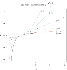
We next introduce a family of stress functions whose attracting and repulsing energies follow power laws, in analogy to Noack’s generalized energy functions for graph drawing (Noack, 2003, 2007, 2009). However, we would like this family to also include logarithmic laws, as in Noack’s “LinLog” energy (Noack, 2003, 2007). To accommodate logarithms in the family of power transformations, statisticians have long used the so-called Box-Cox family of transformations, defined ford>0 by

BCα(d) =

_dα₋₁

α (α6=0),

log(d) (α=0).

This modification of the raw power transformationsdα not only affords analytical fill-in with the natural logarithm forα=0, it also extends the family toα<0 while preserving increasing mono-tonicity of the transformations: forα_{<0 raw powersd}α

are decreasing whileBCα(d)is increasing.

The derivative is

BCα′(d) = dα−1>0 ∀d>0, ∀α∈IR.

By subtracting the (otherwise irrelevant) constant 1 in the numerator and dividing byα, Box-Cox transformations are affinely matched to the natural logarithm atd=1 for all powersα:

BCα(1) =0, BCα′(1) =1.

See Figure 1 for an illustration of Box-Cox transformations.

Using Box-Cox transformations we construct a generalization of Kruskal’s stress function by allowing arbitrary power laws for the attracting and the repulsing energies, subject to the constraint that the attracting power is greater than the repulsing power to guarantee that the minimum com-bined energy is finite (>₋∞). We denote the attracting power byµ+λand the repulsing power by

µwith the understanding thatλ>0 and₋∞<µ<+∞.

Definition 1 TheB-C family of stress functionsfor complete distance data D= (Di j)i,j is given

by

S(d_|D) =

_∑

i,j=1,...,N

Di,j ν

BCµ+λ(di,j) − Di,j λ

BCµ(di,j)

. (1)

As we assumeDi,j>0 fori6= jthe weight termDi,jνis meaningful for all powers−∞<ν<

+∞. ThusDi,jν upweights the summands for largeDi,j whenν>0 and downweights them when ν<0; forν=0 the stress function is an unweighted sum. The parameterνallows us to capture a couple of extant stress functions; see Table 1. Kruskal’s stress function does not require ν_{as it} arises fromµ=1,λ=1 andν=0. The idea of using general power laws in an attraction-repulsion paradigm arose independently in the first author’s PhD thesis (Chen, 2006) and in Noack (2009). For a discussion of the relationship between the two proposals see Section 2.5.

2.3 Edgewise Unbiasedness of Stress Functions

The reason for introducing the multiplier Di,jλ in the repulsing energy is to grant what we call edgewise unbiasedness: If there exist only two objects, N=2, with target distanceD, then the stress functionS(d) =Dν BCµ+λ(d)−DλBCµ(d)

should be minimized byd=D:

D = argmin_dDν

BCµ+λ(d)−DλBCµ(d)

1 2 3 4

−4

−2

0

2

4

Box−Cox Transformations: y==x

µ µ₋₋₁

µ µ

x

y

µ µ ==3

µ µ ==2

µ µ ==1

µ µ ==0

µ µ ==−1

µ µ ==−2

Figure 1: Box-Cox Transformations:y=xµ₋₁

µ

This property is easily verified usingλ>0: S′(d) =Dν+µ−1 dλ₋Dλ, henceS′(d)<0 ford_∈ (0,D)andS′(d)>0 ford_∈(D,∞), so thatS(d)is strictly descending on(0,D)and strictly ascend-ing on(D,∞). This property holds only for this particular choice of the powerDλin the repulsing energy term.

Edgewise unbiasedness is essential to grant the following exact reconstruction property:

Proposition 2 If the target data Di,jform a set of Euclidean distances in the embedding dimension,

Di,j=kxi−xjk(i,j=1, ...,N), then all B-C stress functions are minimized by the embeddings that

reproduce the target distances exactly: di,j=Di,j.

Note that embeddings are unique only up to rotations, translations and reflections. They may have additional non-uniqueness properties that may be peculiar to the data.

2.4 Scale Sensitivity

of what is really just dissimilarity data, or due to intrinsic higher dimensionality of the underlying objects. To gain insight into the nature of the compromises, it is beneficial to construct a simple paradigmatic situation in which contention between conflicting distance data can be analyzed. One such situation is as follows: Assume again that there are only two objects (N=2), but that target distances were obtained twice for this same pair of objects, resulting in different valuesD1andD2

(due to observation error, say). In practice, one often reduces multiple distances by averaging them, but a more principled approach is to form a stress function with multiple stress terms per object pair

(i,j). In general, if target distancesDi,j,k for the object pair(i,j)are observedKi,j times, the B-C stress function will be

S =

_∑

i,j=1,...,N

∑

k=1,...,Ki,j Di,j,kν

BCµ+λ(di,j)−Di,j,kλBCµ(di,j)

.

With this background, the paradigmatic situation of two target distancesD1andD2observed on one object pair is the simplest case that exhibits contention between conflicting distance information. The stress function for the single embedding distancedis

S = D1ν

BCµ+λ(d)−D1λBCµ(d)

+ D2ν

BCµ+λ(d)−D2λBCµ(d)

.

It is minimized by

dmin =

α₁D1λ+α2D2λ

1/λ

, where α₁= D1 ν

D1ν+D2ν

, α₂= D2

ν

D1ν+D2ν

, (2)

so thatα₁+α₂=1. Thusdminis the LebesgueLλnorm of the 2-vector(D1,D2)with regard to the

Bernoulli distribution with probabilitiesα₁andα₂(an improper norm for 0<λ<1). However,α₁ andα₂are also functions of(D1,D2), hence the minimizing distancedmin=d(D1,D2)is a function of the target distances in a complex way. Yet, the Lebesgue norm interpretation is useful because it allows us to analyze the dependence ofdon the parametersλ_andν_separately:

• For fixed D1₆=D2, the minimizing distance d is a monotone increasing function ofν for

−∞<ν<∞, and we have

dmin =

α₁D1λ+α2D2λ

1/λ ↑ _max(D1,D2) _as ν↑∞,

↓ min(D1,D2) as ν↓ −∞.

The reason is that ifD1>D2we haveα_1↑1 asν_↑∞, andα_2↑1 asν_{↓ −}∞.

• For fixed D16=D2, the minimizing distance d is a monotone increasing function of λ for

0<λ_<∞_{, and we have}

dmin = α_1D1λ+α_2D2λ1/λ

↑ max(D1,D2) as λ↑∞, ↓ D1α1_D2α2 _{as λ↓0.}

Conclusion:Embeddings that minimize B-C stress compromise ever more in favor of ... ... larger distances asλ_↑∞orν_↑∞, with full max-dominance in either limit;

... smaller distances asλ_↓0orν_{↓ −}∞, with full min-dominance only in theν-limit.

We use the term “small scale sensitivity” for the behavior of stress functions asλ_{↓0 and/or}ν_↓

−∞. It has the effect of reinforcing local structure because object pairs with small target distances will preferentially be placed close together in the embedding. A related observation was made by Noack (2003) for λ_↓0 in graph drawing and called “clustering strength”; this concept is not identical to small distance sensitivity, however; see Section 2.5.

2.5 Distances versus Weights

Noack (2009) presents a family of “energy functions” for weighted graphs/networks that should be discussed here because it might be thought to be identical to the B-C family of stress functions— which it is not, though there exists a connection. The following discussion is meant to clarify the difference between specifying the relation among object pairs in terms of weights and in terms of distances.

Underlying the idea of mapping weighted graph data to graph drawings is a density paradigm. The intuition is that objects connected by edges with large weights should be represented by em-bedding points that are near each other so as to form high density areas. Hence large weights play a similar role as small distances in their intended effects on embeddings. Weights and distances are therefore in an inverse relation to each other, a fact that will be made precise below.

Next we follow Noack (2009) and consider data given as edge weightswi,j≥0 for all pairs(i,j) with the interpretation that an edge in a graph “exists” between objectsiand jifwi,j>0. (He also allows node weightswi, but we set these to 1 as they add no essential freedom of functional form.) The family of energy functions he considers uses a general form of power laws for attracting and repulsing energies:

U(d_|W) =

_∑

i,j=1,...,N

wi,j

di,ja+1

a+1 −

di,jr+1

r+1 !

, (3)

where we writeW= (wi,j)i,j=1,...,N. It is assumed thata>rin order to grant finitely sized minimiz-ing embeddminimiz-ings for connected graphs. In the spirit, though not the letter, of Box-Cox transforms, Noack imputes natural logarithms fora+1=0 orr+1=0. Unweighted graphs are characterized by wi,j ∈ {0,1}, in which case the total energy (3) amounts to (1) the sum of attracting energies limited to the edges in the graph, and (2) the sum of repulsing energies forallpairs of nodes. This functional form is suggested by traditional energy functions in graph drawing where an attracting force holds the embedding pointsxiandxjtogether if there exists an edge between them and where the repulsing force is pervasive and exists for all pairs so as to disentangle the embedding points by spreading them out.

We now ask how the energy functions (3) and the B-C stress functions (1) relate to each other. A simple answer can be given by drawing on the notion of edgewise unbiasedness: in a two-node situation with single weightw, find the embedding distancedminthat minimizes the energy function

(3); this distance dmin=d(w) can be interpreted as the target distance D for which the energy function is edgewise unbiased. Thus the canonical relation between weights and target distances isD=d(w). For an energy function (3) the specialization to two nodes isU =w da+1_/(a+1)− dr+1/(r+1), whose stationarity condition isU′ =wda₋dr=0, hence w=1/da−r andd(w) =

edgewise unbiased target distanceDis

D = 1

w1/(a−r). (4)

Using the translationwi,j=Di,j−(a−r)and the conventionwi,j =0⇒Di,j = +∞⇒Di,j−(a−r)=0, we can rewrite the energy function (3) modulo irrelevant constants as

U(d_|D) _∼

_∑

i,j=1,...,N

Di,j−(a−r)BCa+1(di,j) − BCr+1(di,j)

. (5)

A comparison with (1) shows that the 2-parameter family of energy functions (5) forms a subfamily of the 3-parameter family of distance-based B-C stress functions (1) as follows:

ν=₋(a₋r), µ=r+1, λ=a₋r.

Thus the essential constraint is that λ=₋ν, entailingν<0. In light of the results of Section 2.4 this constraint implies a counterbalancing of distance sensitivities implied by these parameters: as λ_↑∞ large distance sensitivity increases, but simultaneously ν=₋λ_{↓ −}∞ and hence small scale sensitivity increases as well. Full clarity of the interplay is gained by repeating the exercise of Section 2.4 in the case ν=₋λ: Given two target distances D1 andD2 for N=2 objects, the

minimizing distance is obtained by specializing (2) toν=₋λ:

dmin = 1

1 2D1−

λ +1

2D2− λ1/λ

↓ min(D1,D2) as λ_↑∞,

↑ √D1D2 as λ_↓0.

Thus the minimizing distance dmin is the reciprocal of the Lebesgue Lλ norm of the vector (D1−1_,D2−1_{) with regard to a uniform distribution α}

1=α2=1/2. The identification ν=−λ

has therefore a considerable degree of small scale sensitivity for all values ofλ>0, and counter-intuitively it increases with increasingλ: apparently the increasing small scale sensitivity incurred from the parameterν_{↓ −}∞outweighs the diminished small scale sensitivity due toλ_↑+∞.

It follows that Noack’s notion of “clustering strength” (Noack, 2003) is not identical to our no-tion of small scale sensitivity because clustering strength increases forλ=₋ν_↓0. Rather, clustering strength has to do with the implied translation of a fixed weightwto a target distanceD=1/w1/λ

according to (4): relatively large weightswwill result in relatively ever smaller target distancesD

asλ_↓0, thus reinforcing the clustering effect by the simple translationw_7→D. Diminishing small scale sensitivity forλ=₋ν_↓0 is a lesser effect by comparison.

2.6 B-C Stress Functions for Incomplete Distance Data or Distance Graphs

In order to arrive at stress functions for non-full graphs, we extend a device we used previously to transform Kruskal-Shepard MDS into a localized or graph version called “local MDS” or “LMDS” (Chen and Buja, 2009). We now assume target distancesDi,j are given only for edges(i,j)∈Ein a graph. Starting with stress functions (1) for full graphs, we replace the dissimilaritiesDi,j for non-edges(i,j)_∈/E with a single large dissimilarity D∞which we let go to infinity. We down-weight

these terms with a weightwin such a way thatwD∞λ+ν=tλ+νis constant:

S =

_∑

(i,j)∈E

Di,jν

BCµ+λ(di,j) − Di,jλBCµ(di,j)

+ w

∑

(i,j)∈/E

D∞ν

BCµ+λ(di,j) − D∞λBCµ(di,j)

AsD∞→∞, we havew= (t/D∞)ν+λ→0 andwD∞ν→0, hence in the limit we obtain:

S =

_∑

(i,j)∈E

Di,jν

BCµ+λ(di,j) − Di,jλBCµ(di,j)

− tν+λ

∑

(i,j)∈/E

BCµ(di,j). (6)

This procedure justifies wiping out the attracting energy outside the graph. We call (6) the B-C

family of stress functions for distance graphs. The parametert balances the relative strength of

the combined attraction and repulsion inside the graph with the repulsion outside the graph. For completeness, we list the assumed ranges of the parameters:

t_≥0, λ>0, ₋∞<µ<∞, ₋∞<ν<∞.

An interesting variation of the idea of pervasive repulsion is proposed by Koren and C¸ ivril (2009) who use finite rather than limiting energies.

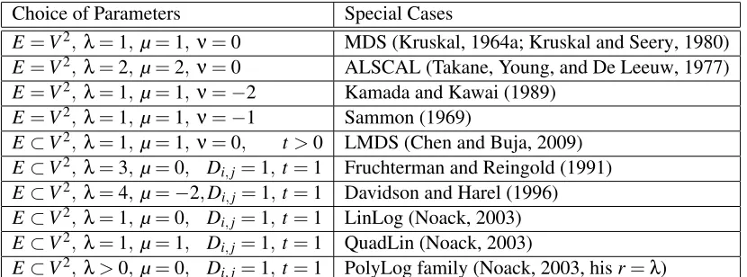
Choice of Parameters Special Cases

E=V2, λ=1,µ=1,ν=0 MDS (Kruskal, 1964a; Kruskal and Seery, 1980)

E=V2, λ=2,µ=2,ν=0 ALSCAL (Takane, Young, and De Leeuw, 1977)

E=V2, λ=1,µ=1,ν=₋2 Kamada and Kawai (1989)

E=V2, λ=1,µ=1,ν=₋1 Sammon (1969)

E_⊂V2, λ=1,µ=1,ν=0, t>0 LMDS (Chen and Buja, 2009)

E_⊂V2, λ_{=3,µ=0, Di,j=1,t=1 Fruchterman and Reingold (1991)}

E⊂V2, λ=4,µ=₋2,Di,j=1,t=1 Davidson and Harel (1996)

E_⊂V2_{, λ=1,µ=0, D}

i,j=1,t=1 LinLog (Noack, 2003)

E_⊂V2, λ=1,µ=1, Di,j=1,t=1 QuadLin (Noack, 2003)

E_⊂V2, λ>0,µ=0, Di,j=1,t=1 PolyLog family (Noack, 2003, hisr=λ)

Table 1: Some special cases of stress functions and their parameters in the B-C family. The first four entries refer to stress functions for complete distance data; the last five entries refer to energy functions for plain graphs (in which caseDi,j=1 for all edges and henceνis vacuous). LMDS applies to incomplete distance data or distance graphs, as do all members of the B-C family. (Not included is the family of power laws for weighted graphs by Noack (2009) because they become stress functions for distance graphs only after a mapping of weights to distances.)

2.7 An Irrelevant Constant: Weighting the Attraction

Noack (2003, Section 5.5) observed that for his LinLog energy function the relative weighting of the attracting energy relative to the repulsing energy is irrelevant in the sense that such weighting would only change the scale of the minimizing layout but not the shape. A similar statement can be made for all members of the B-C family of stress functions. To demonstrate this effect, we introduce B-C stress functions whose attraction is weighted by a factorcλ(c>0):

Sc(d) =

∑

(i,j)∈E

Di,jν

cλBCµ+λ(di,j) − Di,jλBCµ(di,j)

− tν+λ

∑

(i,j)∈/E

whered= (di,j)is the set of all configuration distances for all pairs(i,j), including those not in the graphE. The repulsion terms are still differentially weighted depending on whether(i,j)is an edge of the graphE or not, which is in contrast to most energy functions proposed in the graph layout literature where invariablyt=1.

In analogy to Noack’s argument, we observe the following form of scale equivariance:

S1(c d) = cµSc(d) + const.

As a consequence, ifd is a minimizing set of configuration distances forSc(·), then the distances

c dof the scaled embeddingcXminimize the original unweighted B-C stress functionS1(_·). It is in this sense that Noack’s PolyLog family of stress functions can be considered as a special case of the B-C family: PolyLog energies agree with B-C stress functions for unweighted graphs (Di,j=1) forµ=0 andt=1 up to a multiplicative factor in the attracting energy.

2.8 Unit-Invariant Forms of the Repulsion Weight

In the B-C family of stress functions (6), the relative strength of attracting and repulsing forces is balanced by the parametert. This parameter, however, has two deficiencies: (1) It suffers from a lack of invariance under a change of units in the target distancesDi,j; (2) it has stronger effects in sparse graphs than dense graphs because the number of terms in the summations overEandV_\E

vary with the size of the graphE. Both deficiencies can be corrected by reparametrizingt in terms of a new parameterτas follows:

tλ+ν = |E|

|V2_{| − |E|}· median(i,j)∈EDi,j

λ+ν

·τλ+ν.

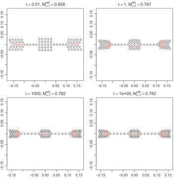
This new parameterτis unit free and adjusted for graph size. (Obviously the median can be replaced with any other statisticS(D)that is positively homogeneous of first order:S(cD) =cS(D)forc>0.) These features enable us to formulate past experience in a problem-independent fashion as follows: in the examples we have tried,τ=1 has yielded satisfactory results. In light of this experience, there may arise few occasions in practice where there is a need to tuneτ. As users work with different units inDi,j or different neighborhood sizes when defining NN-graphs, the recommendationτ=1 stands. Just the same, we will illustrate the effect of varyingτin an artificial example (Section 4.1).

3. Meta-Criteria for Parameter Selection

point to point. The corresponding output neighborhood

N

_d(i)can then be defined as theK(i)-NN set with regard todi,j. The pointwise meta-criterion at thei’th point is defined as size of the overlap between

N

_d(i)and

N

_D(i), hence it is in frequency form

Nd(i) = |

N

d(i)∩

N

D(i)|,

and in proportion form, using_|

N

D(i)|as the baseline,

Md(i) = |

N

_d(i)_∩

N

_D(i)_| |

N

_D(i)_| .

The global meta-criteria are simply the averages over all points:

Nd =

1

|V_|

∑

_i Nd(i) and Md=

1

|V_|

∑

_i Md(i).

Only when all input neighborhood sizes are equal,_|

N

_D(i)_|=K, is there a simple relationship be-tweenNd andMd:Md= _K1Nd. We subscript these quantities withd because they serve to compare different outputs(xi)i=1...N(configurations, embeddings, graph drawings), but all that is used are the interpoint distancesdi,j=kxi−xjk. The proportion formMd is obviously advantageous because it allows comparisons across differentK(orε).

Whether the meta-criterion values are small or large should be judged not against their possible ranges ([0,1]forMd) but against the possibility thatdi,j(hence the embedding) andDi,jare entirely unrelated and generate only random overlap in their respective neighborhoods

N

_d(i)and

N

_D(i). The expected value of random overlap is not zero, however; rather, it is E[_|

N

_d(i)_∩

N

_D(i)_|] =_|

N

_d(i)_{| ·} |

N

D(i)|/(|V|−1)because random overlap should be modeled by a hypergeometric distribution with

|

N

_D(i)_|“defectives” and_|

N

_d(i)_|“draws” from a total of_|V_{| −}1 “items.” The final adjusted forms of the meta-criteria are therefore:

N_dad j(i) = _|

N

d(i)∩

N

D(i)| − 1

|V_{| −}1|

N

d(i)| · |

N

D(i)|,

M_dad j(i) = |

N

d(i)∩

N

D(i)| |

N

_D(i)_| −

1

|V_{| −}1|

N

d(i)|,

N_dad j = 1

|V_|

∑

_i N

ad j

d (d), M ad j

d =

1

|V_|

∑

_i M

ad j d (d).

When the neighborhoods are allK-NN sets,_|

N

_d(i)_|=_|

N

_D(i)_|=K, these expressions simplify:

N_dad j(i) = _|

N

_d(i)_∩

N

_D(i)_{| −} K 2 |V_{| −}1,

M_dad j(i) = |

N

d(i)∩

N

D(i)|

K −

K |V_{| −}1 =

N_dad j(i)

K ,

N_dad j = Nd −

K2

|V_{| −}1, M ad j

d = Md −

K |V_{| −}1 =

N_dad j

K .

Methods that have this invariance are called “non-metric” in proximity analysis/multidimensional scaling because they depend only on the ranks and not the actual values of the distances.

In what follows, we will reportMad j_d for each configuration shown in the figures, and we will also use the pointwise values Md(i) as a diagnostic by highlighting points withMd(i)<1/2 as problematic in some of the figures.

Remark 3 Venna and Kaski (2006, and references therein) introduce an interesting distinction be-tween “trustworthiness” and “continuity” measurement. In our notation the points in

N

_d(i)_\

N

_D(i) violate trustworthiness because they are shown near but are not near in truth (near = being in the K(i)-NN), whereas the points in

N

_D(i)_\

N

_d(i)violate continuity because they are near in truth but not shown as near. Venna and Kaski (2006) measure both violations separately based on distance-ranks. We implicitly also measure both, but more crudely by unweighted counting of violations. It turns out, however, that the two violation counts are the same:_|

N

_d(i)_\

N

_D(i)_|=_|

N

_D(i)_\

N

_d(i)_|= K(i)_{− |}

N

_d(i)_∩

N

_D(i)_|. Thus our meta-criterion is simultaneously a measure of trustworthiness and of continuity. Lee and Verleysen (2008) introduce a larger class of potentially interesting meta-criteria that include ours and Venna and Kaski (2006) as special cases.

4. B-C Stress Functions Applied

In this section, we illustrate the methodology with simulated data (Section 4.1), the Olivetti face data (Section 4.2) and the Frey face data (Section 4.3).

4.1 Simulated Data

We introduced three parameters in the B-C stress functions for complete distance data, namely,λ,

µandν, and a fourth parameter,τ, in the B-C stress functions for incomplete distance graph data. In this subsection, we will examine how three of the four parameters affect configurations in terms of their local and global structure by experimenting with an artificial example. We will simplify the task and eliminate the parameterνby setting it to zero, so that the weightDi,jν=1 disappears from the stress functions. The reason for doing so is that both parametersνandλplay a role in determining scale sensitivity, and, while they are not redundant, the weighting powerνis the more dangerous of the two because it can single-handedly destabilize stress functions asν_{↓ −}∞through unlimited outweighting of large distances. By comparison, the small scale sensitivity caused by small values of the parameterλ>0 is limited as the analysis of Section 2.4 shows.

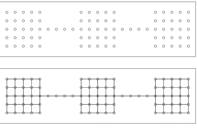
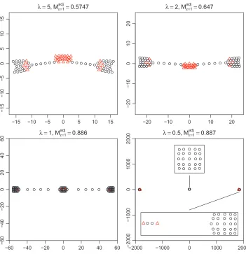
To illustrate the effects of the remaining parametersλ,µandτon embeddings, we constructed an artificial data example consisting of 83 points that form a geometric shape represented in Figure 2 (top). The design was inspired by a simulation example used by Trosset (2006). The distance between any pair of adjacent points is set to 1. To define an initial local graph, as input to the stress functions, we connected each point with its adjacent neighbors with distance 1 (Figure 2, bottom). That is, we used metric nearest neighborhoods with radius 1. Thus, interior points have node degree 4, corner points and connecting points have node degree 2, and the remaining peripheral points have node degree 3. The geometry of this input graph is intended to represent three connected clusters with an internal structure that is relatively tight compared to the connecting structure.

Figure 2: The original configuration (top) and initial local graph (bottom)

2, and a random start, respectively. Starting from the true input configurations is of course not actionable in practice, but it serves a purpose: it demonstrates the biases and distortions implied by minimization of the stress function under the best of circumstances. Starting from a random configuration, on the other hand, gives indications about the stability of the solutions in terms of local minima, as well as the effort required to get from an uninformed starting configuration to a meaningful local minimum. (In practice, one never knows how truly optimal any configuration is that has been obtained by a numerical algorithm, and a better sense of the issue is often obtained only by analyzing the solutions obtained from multiple restarts.)

For starts from the input configurations, the results are shown in Figures 3, 5, and 7, and for starts from random configurations they are shown in Figures 4, 6, and 8, along with their Mad j values that measure the local faithfulness of the configuration. We also colored red (symbolled triangles) the points whose neighborhood structure is not well preserved in terms of a proportion <1/2 of shared neighbors between input and output configurations (M(i)<1/2).

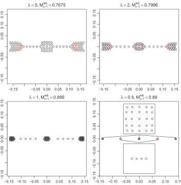
Parameterλ: We setµ=0 andτ=1 and letλvary as follows:λ=5, 2, 1, 0.5. The resulting configurations are shown in Figures 3 and 4. The overall observation from both figures is that for smallerλthe greater small-scale sensitivity causes the configurations to cluster more strongly. We also notice in both figures that Mad j increases with decreasing λ, which indicates local structure within clusters is better recovered when the clusters are well separated. To confirm this, we show a zoom on the nearly collapsed points in the bottom right configurations and observe the square structure in the input configuration is almost perfectly recovered. This indicates that by tuningλ properly the resulting configurations can reveal both macro structure in terms of relative cluster placement as well as micro structure within each cluster.

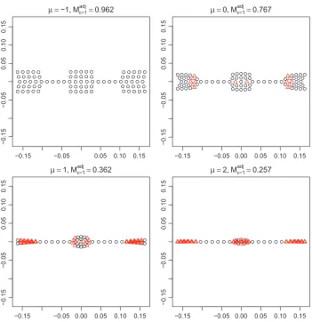
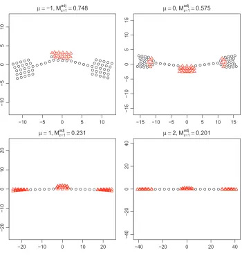
Parameter µ: In Figures 5 and 6, we examine the effect ofµ. We fixλ=5 andτ=1 and letµ

−0.15 −0.05 0.00 0.05 0.10 0.15

−0

.1

5

−0

.0

5

0

.0

5

0

.1

0

0

.1

5

λ =5, M_ε=1

adj

=0.7675

−0.15 −0.05 0.00 0.05 0.10 0.15

−0

.1

5

−0

.0

5

0

.0

5

0

.1

0

0

.1

5

λ =2, M_ε=1

adj

=0.7996

−0.15 −0.10 −0.05 0.00 0.05 0.10 0.15

−0

.1

5

−0

.0

5

0

.0

0

0

.0

5

0

.1

0

0

.1

5 λ =1, Mε=1

adj

=0.886

−0.15−0 −0.10 −0.05 0.00 0.05 0.10 0.15

.1

5

−0

.1

0

−0

.0

5

0

.0

0

0

.0

5

0

.1

0

0

.1

5 λ =0.5, Mε=1

adj

=0.89

Figure 3: The configurations with varyingλwith other parameters fixed atµ=0, τ=1, starting from the input configuration (Figure 2).

−15 −10 −5 0 5 10 15

−1

5

−1

0

−5

0

5

1

0

1

5

λ =5, M_ε=1

adj

=0.5747

−20 −10 0 10 20

−2

0

−1

0

0

1

0

2

0

λ =2, M_ε=1

adj

=0.647

−60 −40 −20 0 20 40 60

−6

0

−4

0

−2

0

0

2

0

4

0

6

0 λ =1, Mε=1

adj

=0.886

−2000−2 −1000 0 1000 2000

0

0

0

−1

0

0

0

0

1

0

0

0

2

0

0

0 λ =0.5, Mε=1

adj

=0.887

Figure 4: The configurations with varyingλwith other parameters fixed atµ=0, τ=1, starting from a random configuration.

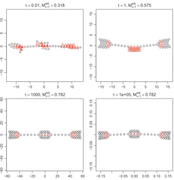
Parameter τ: We fixλ=5 and µ=0 and varyτ as follows: τ= 0.01, 1, 103, 105. The

−0.15 −0.05 0.05 0.10 0.15

−0

.1

5

−0

.0

5

0

.0

5

0

.1

0

0

.1

5

µ =−1, M_ε=1

adj

=0.962

−0.15 −0.05 0.00 0.05 0.10 0.15

−0

.1

5

−0

.0

5

0

.0

5

0

.1

0

0

.1

5

µ =0, M_ε=1

adj

=0.767

−0.15 −0.05 0.00 0.05 0.10 0.15

−0

.1

5

−0

.0

5

0

.0

5

0

.1

0

0

.1

5

µ =1, M_ε=1

adj

=0.362

−0.15 −0.05 0.00 0.05 0.10 0.15

−0

.1

5

−0

.0

5

0

.0

5

0

.1

0

0

.1

5

µ =2, M_ε=1

adj

=0.257

Figure 5: The configurations with varyingµwith other parameters fixed atλ=5, τ=1, starting optimization from the input configuration (Figure 2).

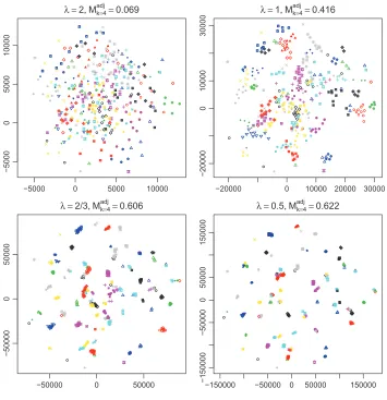
4.2 Olivetti Faces Data

This data set, published on Sam Roweis’ website_{http://www.cs.toronto.edu/˜roweis/data.}

html, contains 400 facial images of 40 people, 10 images for each person. All images are of size 64 by 64. Mathematically, each image can be represented by a long vector, each element of which records the light intensity of one pixel in the image. Given this representation, we treat each image as a data point lying in a 4096-dimensional space (64_×64 = 4096). For visualization purposes we reduce the dimension from 4096 to 2. As the 40 faces form natural groups, we would expect effective dimension reduction methods to show clusters in their configurations. If this expectation is correct, then this data set provides an excellent test bed for the effect of the clustering powerλ.

−10 −5 0 5 10

−1

0

−5

0

5

1

0

µ =−1, M_ε=1

adj

=0.748

−15 −10 −5 0 5 10 15

−1

5

−1

0

−5

0

5

1

0

1

5

µ =0, M_ε=1

adj

=0.575

−20 −10 0 10 20

−2

0

−1

0

0

1

0

2

0

µ =1, M_ε=1

adj

=0.231

−40 −20 0 20 40

−4

0

−2

0

0

2

0

4

0

µ =2, M_ε=1

adj

=0.201

Figure 6: The configurations with varyingµwith other parameters fixed atλ=5, τ=1, starting from a random configuration.

we connected each point to its four nearest neighbors. In the resulting graph five small components were disconnected from the main component of the graph. Each of them contained images from a single person, with 5 images for one person and 5 images for another four persons. Since the disconnected components are trivially pushed away from the main component in any embedding due to the complete absence of attraction, we discarded them and kept the 355 images representing 36 people for further analysis. We created for each person a unique combination of color and symbol to code the points representing it.

−0.15 −0.05 0.05 0.10 0.15

−0

.1

5

−0

.0

5

0

.0

5

0

.1

0

0

.1

5

τ =0.01, M_ε=1

adj

=0.858

−0.15 −0.05 0.00 0.05 0.10 0.15

−0

.1

5

−0

.0

5

0

.0

5

0

.1

0

0

.1

5

τ =1, M_ε=1

adj

=0.767

−0.15 −0.05 0.00 0.05 0.10 0.15

−0

.1

5

−0

.0

5

0

.0

5

0

.1

0

0

.1

5

τ =1000, M_ε=1

adj

=0.782

−0.15 −0.05 0.00 0.05 0.10 0.15

−0

.1

5

−0

.0

5

0

.0

5

0

.1

0

0

.1

5

τ =1e+05, M_ε=1 adj

=0.782

Figure 7: The configurations with varyingτwith other parameters fixed atλ=5, µ=0, starting from the input configuration (Figure 2).

produce exactly 36 clusters: some images of different people are not quite distinguishable in the configurations and some images of the same person are torn apart. The former could really present similar images; the latter could be due to the placement of images in the random start. However, the overall impression is to confirm the clustering effect due to small scale sensitivity for small values of λ. An interesting observation is that the meta-criterionMad j_k increases as the small scale sensitivity strengthens, which assures us of the faithfulness of local topology.

−10 −5 0 5 10

−1

0

−5

0

5

1

0

τ =0.01, M_ε=1

adj

=0.318

−15 −10 −5 0 5 10 15

−1

5

−1

0

−5

0

5

1

0

1

5

τ =1, M_ε=1

adj

=0.575

−60 −40 −20 0 20 40 60

−6

0

−4

0

−2

0

0

2

0

4

0

6

0 τ =1000, Mε=1

adj

=0.782

−0.15 −0.05 0.00 0.05 0.10 0.15

−0

.1

5

−0

.0

5

0

.0

5

0

.1

0

0

.1

5

τ =1e+05, M_ε=1 adj

=0.782

Figure 8: The configurations with varyingτwith other parameters fixed atλ=5, µ=0, starting from a random configuration.

K=4; LLE configurations degenerated to lines or lines and a big cluster when K = 4 and 6, respectively.

4.3 Frey Face Data

● ● ● ● ● ● ● ● ● ● ● ● ● ● ● ● ● ● ● ● ● ● ● ● ● ● ● ● ● ● ● ● ● ● ● ● ● ● ● ● ● ● ● ● ●

−5000 0 5000 10000

−5 0 0 0 0 5 0 0 0 1 0 0 0 0

λ =2, Mk=4

adj =0.069 ● ● ● ● ● ● ● ● ● ● ● ● ●●● ● ● ● ● ● ● ● ● ● ● ● ● ● ● ● ● ● ● ● ● ● ●● ● ● ● ● ● ● ●

−20000 0 10000 20000 30000

−2 0 0 0 0 0 1 0 0 0 0 3 0 0 0

0 λ =1, Mk=4

adj =0.416 ● ● ●●● ● ● ● ● ● ● ● ●●● ● ● ● ● ● ● ● ● ● ● ● ● ●● ● ● ● ● ● ● ● ●● ● ● ● ● ● ● ●

−50000 0 50000

−5 0 0 0 0 0 5 0 0 0 0

λ =2/3, Mk=4

adj =0.606 ● ● ●●● ● ● ●● ● ● ● ●●● ● ● ● ● ●● ● ● ● ● ●● ●●● ●●●● ● ● ● ● ● ● ● ● ● ● ●

−150000−1 −50000 0 50000 150000

5 0 0 0 0 −5 0 0 0 0 0 5 0 0 0 0 1 5 0 0 0 0

λ =0.5, Mk=4

adj

=0.622

Figure 9: Olivetti Faces. Configurations with varyingλwith other parameters fixed atµ=0,τ=1.

dimensional embeddings. The fact is that the intrinsic structure of the full data set is well preserved in this subset, partly due to the inherent redundancies in video sequences: the images close in order are very similar because the stills are taken more frequently than Frey’s facial expression changes.

In Figure 11 we show the first two principal components of the 3D configurations for varying

● ● ● ● ● ● ● ● ● ● ● ● ● ●● ● ●● ● ● ● ● ● ● ● ● ● ● ● ● ● ● ● ● ● ● ● ● ● ● ● ● ● ● ●

−3000−3 −1000 0 1000 2000 3000

0 0 0 −1 0 0 0 0 1 0 0 0 2 0 0 0 3 0 0

0 PCA, Mk=4

adj =0.143 ● ● ● ● ● ● ● ● ● ● ● ● ● ● ● ● ● ● ● ● ● ● ● ● ● ● ● ● ● ● ● ● ● ● ● ● ● ● ● ● ● ● ● ● ●

−3000 −1000 0 1000 2000 3000

−3 0 0 0 −1 0 0 0 0 1 0 0 0 3 0 0 0

MDS, Mk=4 adj =0.177 ● ●● ●● ● ● ● ●● ● ● ● ●● ● ●● ● ● ● ● ● ● ● ●● ● ● ● ● ● ● ● ● ● ● ● ● ● ● ● ● ● ●

−10000 −5000 0 5000 10000

−1 0 0 0 0 −5 0 0 0 0 5 0 0 0 1 0 0 0 0

Isomap, Mk=4 adj =0.249 ● ● ● ●● ● ●● ● ● ● ● ● ●● ●● ●●● ●● ● ● ● ● ● ● ● ● ● ● ● ● ● ● ● ● ● ●● ● ● ● ●

−0.2 −0.1 0.0 0.1 0.2

−0 .2 −0 .1 0 .0 0 .1 0 .2

LLE, Mk=4 adj

=0.269

Figure 10: Olivetti Faces. Configurations from PCA, MDS, Isomap and LLE.

structure, though, is better reflected in the configurations with smaller values ofµ, as suggested by the values of meta-criteria.

5. Summary and Discussion

−0.05 0.00 0.05

−0

.0

5

0

.0

0

0

.0

5

µ =−1, M6

adj

=0.536

−0.05 0.00 0.05

−0

.0

5

0

.0

0

0

.0

5

µ =0, M6

adj

=0.493

−0.05 0.00 0.05

−0

.0

5

0

.0

0

0

.0

5

µ =1, M6

adj

=0.382

−0.10 −0.05 0.00 0.05

−0

.1

0

−0

.0

5

0

.0

0

0

.0

5

µ =2, M6

adj

=0.318

Figure 11: Frey Face Data. Configurations with varyingµwhenλ=1.

The parameters of the proposed family have the following interpretations:

• λ: This parameter determines the relative strengths of the attracting and repulsing forces to each other, while maintaining “edgewise unbiasedness” of the stress function. In practical terms, this parameter strongly influences “small scale sensitivity”: For decreasingλ, it in-creases the small-scale sensitivity, that is, the tendency to group together nearby points in the embedding. Range:λ>0.

• µ: This parameter is the power law of the repulsing energy. The greater µ, the greater is the tendency to suppress large discrepancies between inputs Di,j and outputs di,j. Range:

−∞<µ<+∞.

• τ: A regularization parameter that stabilizes configurations for incomplete distance data, that is, distance graphs, at the cost of some bias (stretching of configurations), achieved by imput-ing infinite input distances with infinitesimal repulsion. Range:τ>0.

The power laws for attracting and repulsing energies are interpreted as Box-Cox transformations, which has two benefits: (1) Box-Cox transformations encompass a logarithmic attracting law for

µ+λ=0 and a logarithmic repulsing law forµ=0; (2) they permit negative powers for both laws because the Box-Cox transformations are monotone increasing for powers in the whole range of real numbers. The regularization parameterτplays a role only when the input distance matrix is incomplete, as in the case of a distance graph or in the case of localization by restricting the loss function to small scale (as in LMDS; Chen and Buja, 2009).

The problem of incomplete distance information is often solved by completing it with addi-tive imputations provided by the shortest-path algorithm, so that MDS-style stress functions can be used—the route taken by Isomap (Tenenbaum et al., 2000). The argument against such completion is that stress functions tend to be driven by the largest distances, which are imputed and hence noisy. Conversely the argument against not completing is that the use of pervasive repulsion to stabilize configurations amounts to imputation also, albeit of an uninformative kind. A full understanding of the trade-offs between completion and repulsion is currently lacking, but practitioners can mean-while experiment with both approaches and compare them on their data. In both cases the family of loss functions proposed here offers control over the scale sensitivity parameterλ, the repulsion powerµ, and the weighting powerν.

Another issue with distance-based approaches is that there is often much freedom in choos-ing the distances, in particular when applied to dimension reduction. There is therefore a need to systematize the choices and provide guidance for “distance selection.”

Appendix A. Stress Minimization

Minimizing stress functions can be a very high-dimensional optimization problem involving all co-ordinates of all points in an embedding, amounting toN pparameters. For this reason, minimization algorithms tend to be based on simple gradient descent (Kruskal, 1964b) or on majorization (Borg and Groenen, 2005). We limit ourselves in this appendix to providing gradients, though with one in-novation to solve the following problem: optimization of stress functions tends to spend much effort on getting the size of the embedding right, which is not only unnecessary but also may cause delay of convergence when in fact the shape of the embedding is already optimized, or misjudgement of convergence when the size has been gotten right but the shape has not. This appendix proceeds therefore in three steps: Section A.1 provides gradients for plain stress functions as presented in the body of this article; Section A.2 derives size-invariant versions of stress functions; Section A.3 provides gradients for the latter. (In order to make the formulas more readable, we set the parameter νto zero and hence ignore it; it would be a simple matter to put it back in the formulas.)

A.1 Gradients for Stress Functions

stress function forµ6=0 andµ+λ₆=0 (butν=0) is

S(x1,···,xN) =

∑

(i,j)∈E

di,jµ+λ−1

(µ+λ₎ −Di,j

λdi,jµ−1

µ

!

−tλ

∑

(i,j)∈EC

di,jµ−1

µ .

Let∇S= (∇₁,_···,∇_N)T _{be the gradient of the stress function with respect toX:} ∇_i= ∂S

∂xi

=

_∑

j∈ND(i)

di,jµ+λ−2−Di,jλdi,jµ−2

(xi−xj)

−tλ

∑

j_∈Nc D(i)

di,jµ−2(xi−xj).

Define aN×NmatrixMas follows:

Mi j=

di,jµ+λ−2−Di,jλdi,jµ−2 if j∈E(i),

−tλdi,jµ−2 if j∈/E(i). Note thatMis symmetric. The gradient can be simplified to

∇_i= ∂S

∂xi

=

_∑

j

Mji(xi−xj)

= (

_∑

j

Mji)xi−

∑

j

Mjixj,

and

∇_S=X_∗(M_·E)₋M_·X,

where E is a N_×d matrix with all elements being 1. The symbol ‘_∗’ represents elementwise multiplication of the two matrices of the same size, and the symbol ‘_·’ stands for regular matrix multiplication.

A.2 Size-Invariant Forms of B-C Stress Functions

As mentioned, it is a common experience that algorithms for minimizing stress functions spend much effort on getting the size of the embedding right. Size, however, is not of interest—shape is. We have therefore a desire to re-express stress in a manner that is independent of size. Fortunately, there exists a general method that achieves this goal: For any configuration, minimize stress with regard to size and replace the original stress with its size-minimized value. This works because the minimization with regard to size can be carried out explicitly with elementary calculus. The result is a new form of stress that is minimized by the same shapes as the original stress, but it is independent of size and hence purely driven by shape. The computational advantage of size-invariant stress is that gradient-based optimization descends along directions that change shape, not size. We sketch the derivation (again forν=0 for less unwieldy formulas).

It is convenient to collect the repulsion terms inside and outside the graph because they share the power law:

S =

_∑

(i,j)∈E

BC_µ+λ(di,j) −

∑

(i,j)∈V2

˜

where

˜

Di,j=

Di,j, (i,j)∈E,

t (i,j)_∈/E.

Next, consider a configurationX= (xi)i=1...N and resized versionssX= (s xi)i=1...Nthereof (s>0). The configuration distances scale along with size: di,j(sX) =s di,j(X). To find the stationary size factorsof the stress as a function ofs,S=S(s), we observe that

∂

∂sBCµ(s di,j) = s

µ₋1_d

i,jµ (∀µ∈IR).

In particular, this holds even forµ=0. Next we solve the stationary equation and check second derivatives:

S(sd) =

_∑

E

BCµ+λ(s di,j) −

∑

V2

˜

Dλ_i,j BCµ(s di,j),

S′(sd) = sµ+λ−1Tden − sµ−1Tnum, (7)

S′′(sd) = (µ+λ₋1)_sµ+λ−2_Tden − (µ−₁)_sµ−1_Tnum, ₍₈₎

whereTden=Tden(d)andTnum=Tnum(d)are defined ford= (di,j)by

Tden=

∑

E

di,jµ+λ, Tnum=

∑

V2

˜

Dλ_i,j di,jµ.

Again (7) and (8) hold even forµ=0 and µ+λ=0. The stationary size factors_∗ that satisfies

S′(s_∗) =0 is

s_∗ =

Tnum

Tden λ

(_∀µ_∈IR, λ>0). (9)

The factors_∗is a strict minimum:

S′′(s_∗d) = λT

λµ+1−2λ num

T_denλµ−2λ > 0 (∀µ∈IR,

λ>0).

EvaluatingS(s_∗)we arrive at asize-invariantyetshape-equivalentform of the stress function. For the evaluation we need to separate power laws from the two logarithmic cases:

S(sd) _≈



 

 

1

µ+λsµ+ λ_T

den − 1_µ sµTnum (µ+λ6=0, µ6=0),

|E_|log(s) + ∑_E log(di,j) − 1_µ sµTnum (µ+λ=0), λsλTden − ∑V2D˜λ_i,j (log(s) +log(d_i,j)) (µ=0),

where “_≈” means “equal up to additive constants that are irrelevant for optimization.” We calculate ˜

S=S(s_∗)separately in the three cases withs_∗from (9):

• µ+λ₆=0,µ₆=0: Several algebraic simplifications produce the following.

˜

S =

1

µ+λ−

1

µ

Tnumλµ+1

T_denλµ =

1

µ+λ−

1

µ

∑_V2D˜λ_i,jd_i,jµ

λµ+1

∑_Edi,jµ+λ

λµ . (10)

[Note that ˜Sgets minimized, hence the ratio on the right gets minimized when the left factor is positive (i.e.,µ<0<µ+1/λ), and it gets maximized when the left factor is negative (i.e.,

• µ+λ=0: We take advantage of the fact thatTden=|E|andµ=−λ. We have

˜

S _{≈ |}E_|λlog

∑

V2

_˜

Di,j

di,j λ

+

_∑

E

log(di,j).

• µ=0: We take advantage of the fact thatTden=∑Edi,jλ and also thatTnum=∑V2D˜λ_i,j is a

constant for optimization with regard tod= (di,j), and any additive term that is just a function of ˜Di,jbut notdi,jcan be neglected. We have

˜

S _≈ λ

_∑

V2

˜

Dλ_i,j

!

log(

_∑

E

di,jλ) −

∑

V2

˜

Dλ_i,jlog(di,j).

Even though size-invariance holds by construction, one checks it easily in all three cases: ˜S(s d) =

˜

S(d).

A.3 Gradients for Size-Invariant Stress Functions

To describe the gradient of the size-invariant stress function ˜S(d). We only consider the caseµ+λ₆=

0 andµ₆=0, which is shown in Equation (10).

Let ∇S = ((∇S)₁, ...,(∇S)_n)T be the gradient the ˜S(d) with respect to configuration

X= (x1, ...,xn)T. We have

(∇S)_i=

1

µ+λ−

1

µ

"

(λµ+1)

Tnum

Tden λµ

(∇Tnum)i−(λµ)

Tnum

Tden λµ+1

(∇Tden)i #

,

(∇Tnum)_i=

∂Tnum(d) ∂xi

=µ

∑

j ˜

Di,jdiµ,−j2(xi−xj),

(∇Tden)_i=

∂Tden(d) ∂xi

= (µ+λ)

_∑

j∈E(i)

d_iµ_,+_jλ−2(xi−xj).

Plug(∇Tnum)iand(∇Tden)i into the(∇S)i, and we have

(∇S)_i=

Tnum

Tden λµ

Tnum

Tden _j∈

∑

_E(i)

d_iµ_,+_jλ−2(xi−xj)−

∑

j

˜

Di,jd_iµ_,−_j2(xi−xj) ! = Tnum Tden λµ

∑

j∈E(i)

Tnum

Tden

d_iµ_,+_jλ−2₋Dλ_jid_iµ_,−_j2

(xi−xj)−

∑

j∈Ec_(i)

t d_iµ_,−_j2(xi−xj) !

.

Define aN_×NmatrixMby

Mi j = 





Tnum

Tdend

µ+1

λ−2

i,j −Di,jλdiµ,−j2

for j_∈E(i),

The gradient can be simplified to

(∇S)_i=

Tnum

Tden λµ

∑

j

Mi j(xi−xj)

=

Tnum

Tden λµ

∑

j

Mi jxi−

∑

j

Mi jxj !

,

and

∇S=

Tnum

Tden λµ

(X_∗(M_·E)₋M_·X).

We did the calculation separately forµ=0 andλ+µ=0 which resulted in the following:

µ=0 : S˜(d)_∼λ

_∑

(i,j)∈V2

˜

Di j !

log

∑

(i,j)∈E

Di,jλ !

−

∑

(i,j)∈V2

˜

Di jlogDi,j,

µ+λ=0 : S˜(d)_∼λ

_∑

(i,j)∈E !

log

∑

(i,j)∈V2

˜

Di jDi,jµ !

+

_∑

(i,j)∈E

logDi,j.

References

Ulas Akkucuk and J. Douglas Carroll. PARAMAP vs. Isomap: A comparison of two nonlinear mapping algorithms. Journal of Classification, 23(2):221–254, 2006.

Ingwer Borg and Patrick J.F. Groenen.Modern Multidimensional Scaling: Theory and Applications. Springer-Verlag, 2005.

Lisha Chen. Local Multidimensional Scaling for Nonlinear Dimension Reduction, Graph Layout

and Proximity Analysis. PhD thesis, Ph.d. Thesis, University of Pennsylvania, Philadelphia,

Pennsylvania, 2006.

Lisha Chen and Andreas Buja. Local multidimensional scaling for nonlinear dimension reduction, graph drawing, and proximity analysis. Journal of the American Statistical Association, 104 (485):209–219, 2009.

Ron Davidson and David Harel. Drawing graphs nicely using simulated annealing. ACM

Transac-tions on Graphics (TOG), 15(4):301–331, 1996.

Thomas M.J. Fruchterman and Edward M. Reingold. Graph drawing by force-directed placement.

Software: Practice and Experience, 21(11):1129–1164, 1991.

Emden Gansner, Yehuda Koren, and Stephen North. Graph drawing by stress majorization. In

Graph Drawing, pages 239–250. Springer, 2005.

Tomihisa Kamada and Satoru Kawai. An algorithm for drawing general undirected graphs.

Infor-mation Processing Letters, 31(1):7–15, 1989.

Joseph B. Kruskal. Multidimensional scaling by optimizing goodness of fit to a nonmetric hypoth-esis. Psychometrika, 29(1):1–27, 1964a.

Joseph B. Kruskal. Nonmetric multidimensional scaling: A numerical method. Psychometrika, 29 (2):115–129, 1964b.

Joseph B. Kruskal and Judith B. Seery. Designing network diagrams. InProc. First General

Con-ference on Social Graphics, pages 22–50, 1980.

John A. Lee and Michel Verleysen. Rank-based quality assessment of nonlinear dimensionality re-duction. In16th European Symposium on Artificial Neural Networks (ESANN), Bruges, Belgium, pages 49–54, 2008.

Fan Lu, S¨und¨uz Keles¸, Stephen J Wright, and Grace Wahba. Framework for kernel regularization with application to protein clustering. Proceedings of the National Academy of Sciences of the

United States of America, 102(35):12332–12337, 2005.

Andreas Noack. Energy models for drawing clustered small world graphs. Technical report, Inst. of Computer Science, Brandenburg Technical University, Cottbus, Germany, 2003.

Andreas Noack. Energy models for graph clustering. Journal of Graph Algorithms and Applica-tions, 11(2):453–480, 2007.

Andreas Noack. Modularity clustering is force-directed layout. Physical Review E, 79(2):026102, 2009.

Sam T. Roweis and Lawrence K. Saul. Nonlinear dimensionality reduction by locally linear embed-ding. Science, 290(5500):2323–2326, 2000.

John W. Sammon. A nonlinear mapping for data structure analysis.IEEE Transactions on Comput-ers, 100(5):401–409, 1969.

Bernhard Sch¨olkopf, Alexander Smola, and Klaus-Robert M¨uller. Nonlinear component analysis as a kernel eigenvalue problem. Neural Computation, 10(5):1299–1319, 1998.

Yoshio Takane, Forrest W. Young, and Jan De Leeuw. Nonmetric individual differences multidimen-sional scaling: An alternating least squares method with optimal scaling features.Psychometrika, 42(1):7–67, 1977.

Joshua B. Tenenbaum, Vin De Silva, and John C. Langford. A global geometric framework for nonlinear dimensionality reduction. Science, 290(5500):2319–2323, 2000.

Michael W. Trosset. Classical multidimensional scaling and laplacian eigenmaps. Presentation given at the 2006 Joint Statistical Meeting (Session 411), 2006.

Jarkko Venna and Samuel Kaski. Local multidimensional scaling.Neural Networks, 19(6):889–899, 2006.