Confidence Intervals and Hypothesis Testing for
High-Dimensional Regression
Adel Javanmard [email protected]
Department of Electrical Engineering Stanford University
Stanford, CA 94305, USA
Andrea Montanari [email protected]
Department of Electrical Engineering and Department of Statistics Stanford University
Stanford, CA 94305, USA
Editor:Nicolai Meinshausen
Abstract
Fitting high-dimensional statistical models often requires the use of non-linear parameter estimation procedures. As a consequence, it is generally impossible to obtain an exact characterization of the probability distribution of the parameter estimates. This in turn implies that it is extremely challenging to quantify theuncertaintyassociated with a certain parameter estimate. Concretely, no commonly accepted procedure exists for computing classical measures of uncertainty and statistical significance as confidence intervals or p-values for these models.
We consider here high-dimensional linear regression problem, and propose an efficient algorithm for constructing confidence intervals andp-values. The resulting confidence inter-vals have nearly optimal size. When testing for the null hypothesis that a certain parameter is vanishing, our method has nearly optimal power.
Our approach is based on constructing a ‘de-biased’ version of regularized M-estimators. The new construction improves over recent work in the field in that it does not assume a special structure on the design matrix. We test our method on synthetic data and a high-throughput genomic data set about riboflavin production rate, made publicly available by B¨uhlmann et al. (2014).
Keywords: hypothesis testing, confidence intervals, LASSO, high-dimensional models, bias of an estimator
1. Introduction
The use of non-linear parameter estimators comes at a price. In general, it is impossible to characterize the distribution of the estimator. This situation is very different from the one of classical statistics in which either exact characterizations are available, or asymp-totically exact ones can be derived from large sample theory (Van der Vaart, 2000). This has an important and very concrete consequence. In classical statistics, generic and well accepted procedures are available for characterizing the uncertainty associated to a certain parameter estimate in terms of confidence intervals orp-values (Wasserman, 2004; Lehmann and Romano, 2005). However, no analogous procedures exist in high-dimensional statistics. In this paper we develop a computationally efficient procedure for constructing confi-dence intervals andp-values for a broad class of high-dimensional regression problems. The salient features of our procedure are:
(i) Our approach guarantees nearly optimal confidence interval sizes and testing power.
(ii) It is the first one to achieve this goal under essentially no assumptions beyond the standard conditions for high-dimensional consistency.
(iii) It allows for a streamlined analysis with respect to earlier work in the same area.
For the sake of clarity, we will focus our presentation on the case of linear regression, under Gaussian noise. Section 4 provides a detailed study of the case of non-Gaussian noise. A preliminary report on our results was presented in NIPS 2013 (Javanmard and Montanari, 2013a), which also discusses generalizations of the same approach to generalized linear models, and regularized maximum likelihood estimation.
In a linear regression model, we are given ni.i.d. pairs (Y1, X1),(Y2, X2), . . . ,(Yn, Xn), with vectors Xi ∈Rp and response variables Yi given by
Yi = hθ0, Xii+Wi, Wi ∼N(0, σ2). (1)
Here θ0 ∈ Rp and h ·,· i is the standard scalar product in Rp. In matrix form, letting Y = (Y1, . . . , Yn)Tand denoting by X the design matrix with rows X1T, . . . , XnT, we have
Y = Xθ0+W , W ∼N(0, σ2In×n). (2)
The goal is to estimate the unknown (but fixed) vector of parametersθ0∈Rp.
In the classic setting, n p and the estimation method of choice is ordinary least squares yielding θbOLS = (XTX)−1XTY. In particular θbOLS is Gaussian with mean θ0 and covarianceσ2(XTX)−1. This directly allows to construct confidence intervals.1
In the high-dimensional setting wherep > n, the matrix (XTX) is rank deficient and one has to resort to biased estimators. A particularly successful approach is the LASSO (Tib-shirani, 1996; Chen and Donoho, 1995) which promotes sparse reconstructions through an
`1 penalty:
b
θn(Y,X;λ)≡arg min θ∈Rp
n 1
2nkY −Xθk
2
2+λkθk1 o
. (3)
1. For instance, lettingQ≡(XTX/n)−1,θbiOLS−1.96σ
p
Qii/n,bθiOLS+ 1.96σ
p
Qii/n] is a 95% confidence
Algorithm 1 Unbiased estimator for θ0 in high-dimensional linear regression models Input: Measurement vectory, design matrixX, parametersλ,µ.
Output: Unbiased estimatorθbu.
1: Letθbn=bθn(Y,X;λ) be the LASSO estimator as per Equation (3).
2: SetΣb ≡(XTX)/n.
3: fori= 1,2, . . . , pdo
4: Let mi be a solution of the convex program:
minimize mTΣbm
subject to kbΣm−eik∞≤µ ,
(4)
whereei ∈Rp is the vector with one at thei-th position and zero everywhere else.
5: SetM = (m1, . . . , mp)T. If any of the above problems is not feasible, then setM = Ip×p.
6: Define the estimator bθu as follows:
b
θu =θbn(λ) + 1
nMX
T(Y −Xbθn(λ)) (5)
In case the right hand side has more than one minimizer, one of them can be selected arbitrarily for our purposes. We will often omit the argumentsY,X, as they are clear from the context.
We denote by S ≡supp(θ0) the support ofθ0∈Rp, defined as supp(θ0)≡ {i∈[p] : θ0,i6= 0},
where we use the notation [p] ={1, . . . , p}. We further lets0≡ |S|. A copious theoretical lit-erature (Cand`es and Tao, 2005; Bickel et al., 2009; B¨uhlmann and van de Geer, 2011) shows that, under suitable assumptions onX, the LASSO is nearly as accurate as if the support
S was knowna priori. Namely, forn= Ω(s0logp), we havekbθn−θ0k22 =O(s0σ2(logp)/n). As mentioned above, these remarkable properties come at a price. Deriving an exact characterization for the distribution ofθbn is not tractable in general, and hence there is no simple procedure to construct confidence intervals andp-values. A closely related property is that θbn is biased, an unavoidable property in high dimension, since a point estimate b
θn ∈ Rp must be produced from data in lower dimension Y ∈
Rn, n < p. We refer to Section 2.2 for further discussion of this point.
In order to overcome this challenge, we construct a de-biased estimator from the LASSO solution. The de-biased estimator is given by the simple formulaθbu =θbn+ (1/n)MXT(Y− Xθbn), as in Equation (5). The basic intuition is thatXT(Y−Xθbn)/(nλ) is a subgradient of the`1 norm at the LASSO solutionθbn. By adding a term proportional to this subgradient, our procedure compensates the bias introduced by the`1 penalty in the LASSO.
We will prove in Section 2.1 thatθbuis approximately Gaussian, with meanθ0and covari-anceσ2(MΣbM)/n, whereΣ = (Xb TX/n) is the empirical covariance of the feature vectors. This result allows to construct confidence intervals andp-values in complete analogy with classical statistics procedures. For instance, letting Q ≡MΣbM, [θbiu−1.96σ
p
Qii/n,θbui + 1.96σpQii/n] is a 95% confidence interval. The size of this interval is of orderσ/
√
is the optimal (minimum) one, i.e., the same that would have been obtained by knowing a priori the support of θ0. In practice the noise standard deviation is not known, butσ can be replaced by any consistent estimatorσb (see Section 3 for more details on this).
A key role is played by the matrix M ∈ Rp×p whose function is to ‘decorrelate’ the columns of X. We propose here to constructM by solving a convex program that aims at optimizing two objectives. One one hand, we try to control |MΣb −I|∞ (here and below
| · |∞ denotes the entrywise `∞ norm) which, as shown in Theorem 8, controls the
non-Gaussianity and bias of θbu. On the other, we minimize [MΣbM]i,i, for each i ∈[p], which controls the variance ofθbiu.
The idea of constructing a de-biased estimator of the form θbu =θbn+ (1/n)MXT(Y − Xθbn) was used by the present authors in Javanmard and Montanari (2013b), that suggested the choiceM =cΣ−1, with Σ =E{X1X1T}the population covariance matrix andca positive constant. A simple estimator for Σ was proposed for sparse covariances, but asymptotic validity and optimality were proven only for uncorrelated Gaussian designs (i.e., Gaussian Xwith Σ = I). Van de Geer, B¨ulhmann, Ritov and Dezeure (van de Geer et al., 2014) used the same construction with M an estimate of Σ−1 which is appropriate for sparse inverse covariances. These authors prove semi-parametric optimality in a non-asymptotic setting, provided the sample size is at least n= Ω((s0logp)2).
From a technical point of view, our proof starts from a simple decomposition of the de-biased estimatorbθu into a Gaussian part and an error term, already used in van de Geer et al. (2014). However, departing radically from earlier work, we realize that M need not be a good estimator of Σ−1 in order for the de-biasing procedure to work. We instead set
M as to minimize the error term and the variance of the Gaussian term. As a consequence of this choice, our approach applies to general covariance structures Σ. By contrast, earlier approaches applied only to sparse Σ, as in Javanmard and Montanari (2013b), or sparse Σ−1 as in van de Geer et al. (2014). The only assumptions we make on Σ are the standard compatibility conditions required for high-dimensional consistency (B¨uhlmann and van de Geer, 2011). A detailed comparison of our results with the ones of van de Geer et al. (2014) can be found in Section 2.3.
1.1 Organization of the Paper Our presentation is organized as follows.
Section 2 considers a general debiased estimator of the formθbu =θbn+ (1/n)MXT(Y − Xθbn). We introduce a figure of merit of the pair M,X, termed the generalized coherence parameterµ∗(X;M). We show that, if the generalized coherence is small, then the debiasing
procedure is effective (for a given deterministic design), see Theorem 6. We then turn to random designs, and show that the generalized coherence parameter can be made as small asp(logp)/n, though a convex optimization procedure for computingM. This results in a bound on the bias ofθbu, cf. Theorem 8: the largest entry of the bias is of order (s0logp)/n. This must be compared with the standard deviation of θbiu, which is of order σ/
√
n. The conclusion is that, for s0 =o(
√
n/logp), the bias of θbu is negligible.
optimal tests can be applied. We prove a general lower bound on the power of our testing procedure, in Theorem 16. In the special case of Gaussian random designs with i.i.d. rows, we can compare this with the upper bound proved in Javanmard and Montanari (2013b), cf. Theorem 17. As a consequence, the asymptotic efficiency of our approach is constant-optimal. Namely, it is lower bounded by a constant 1/ηΣ,s0 which is bounded away from 0,
cf. Theorem 18. (For instanceηI,s0 = 1, andηΣ,s0 is always upper bounded by the condition
number of Σ.)
Section 4 uses the central limit theorem for triangular arrays to generalize the above results to non-Gaussian noise.
Section 5 illustrates the above results through numerical simulations both on synthetic and on real data. In the interest of reproducibility, an Rimplementation of our algorithm is available at http://www.stanford.edu/~montanar/sslasso/.
Note that our proofs require stricter sparsity s0 (or larger sample size n) than required for consistent estimation. We assumes0=o(
√
n/logp) instead ofs0 =o(n/logp) (Cand`es and Tao, 2007; Bickel et al., 2009; B¨uhlmann and van de Geer, 2011). The same assumption is made in van de Geer et al. (2014), on top of additional assumptions on the sparsity of Σ−1.
It is currently an open question whether successful hypothesis testing can be performed under the weaker assumption s0 = o(n/logp). We refer to Javanmard and Montanari (2013c) for preliminary work in that direction. The barrier ats0 =o(
√
n/logp) is possibly related to an analogous assumption that arises in Gaussian graphical models selection (Ren et al., 2013).
1.2 Further Related Work
The theoretical literature on high-dimensional statistical models is vast and rapidly growing. Estimating sparse linear regression models is the most studied problem in this area, and a source of many fruitful ideas. Limiting ourselves to linear regression, earlier work inves-tigated prediction error (Greenshtein and Ritov, 2004), model selection properties (Mein-shausen and B¨uhlmann, 2006; Zhao and Yu, 2006; Wainwright, 2009; Cand`es and Plan, 2009),`2 consistency (Cand`es and Tao, 2005; Bickel et al., 2009). . Of necessity, we do not provide a complete set of references, and instead refer the reader to B¨uhlmann and van de Geer (2011) for an in-depth introduction to this area.
The problem of quantifying statistical significance in high-dimensional parameter esti-mation is, by comparison, far less understood. Zhang and Zhang (2014) and B¨uhlmann (2013) proposed hypothesis testing procedures under restricted eigenvalue or compatibil-ity conditions (B¨uhlmann and van de Geer, 2011). These papers provide deterministic guarantees but, in order to achieve a certain target significance level α and power 1−β, they require |θ0,i| ≥ cmax{σs0logp/ n, σ/
√
n}. The best lower bound (Javanmard and Montanari, 2013b) shows that any such test requires instead |θ0,i| ≥ c(α, β)σ/
√
n. (The lower bound of Javanmard and Montanari 2013b is reproduced as Theorem 17 here, for the reader’s convenience.)
we will propose a test that, for random designs, achieves significance levelαand power 1−β
for|θ0,i| ≥c0(α, β)σ/ √
n.
Lockhart et al. (2014) develop a test for the hypothesis that a newly added coefficient along the LASSO regularization path is irrelevant. This however does not allow to test arbitrary coefficients at a given value of λ, which is instead the problem addressed in this paper. These authors further assume that the current LASSO support contains the actual support supp(θ0) and that the latter has bounded size.
Belloni et al. (2014, 2013) consider inference in a regression model with high-dimensional data. In this model the response variable relates to a scalar main regressor and a p -dimensional control vector. The main regressor is of primary interest and the control vector is treated as nuisance component. Assuming that the control vector is s0-sparse, the au-thors propose a method to construct confidence regions for the parameter of interest under the sample size requirement (s20logp)/n→0. The proposed method is shown to attain the semi-parametric efficiency bounds for this class of models. The key modeling assumption in this paper is that the scalar regressor of interest is random, and depends linearly on the
p-dimensional control vector, with a sparse coefficient vector (with sparsity again of order
o(pn/logp). This assumption is closely related to the sparse inverse covariance assumption of van de Geer et al. (2014) (with the difference that only one regressor is tested).
Finally, resampling methods for hypothesis testing were studied in Meinshausen and B¨uhlmann (2010); Minnier et al. (2011). These methods are perturbation-based procedures to approximate the distribution of a general class of penalized parameter estimates for the case n > p. The idea is to consider the minimizer of a stochastically perturbed version of the regularized objective function, call it ˜θ, and characterize the limiting distribution of the regularized estimator θbin terms of the distribution of ˜θ. In order to estimate the latter, a large number of random samples of the perturbed objective function are generated, and for each sample the minimizer is computed. Finally the theoretical distribution of ˜θ is approximated by the empirical distribution of these minimizers.
After the present paper was submitted for publication, we became aware that Dezeure and B¨uhlmann (2013) had independently worked on similar ideas.
1.3 Preliminaries and Notations
In this section we introduce some basic definitions used throughout the paper, starting with simple notations.
For a matrix A and set of indices I, J, we let AI,J denote the submatrix formed by the rows in I and columns in J. Also, AI,· (resp. A·,I) denotes the submatrix containing just the rows (reps. columns) in I. Likewise, for a vector v, vI is the restriction of v to indices in I. We use the shorthand A−I,J1 = (A−1)I,J. In particular, A−i,i1 = (A−1)i,i. The maximum and the minimum singular values of Aare respectively denoted byσmax(A) and
σmin(A). We write kvkp for the standard `p norm of a vector v, i.e., kvkp = (Pi|vi|p)1/p. and kvk0 for the number of nonzero entries of v. For a matrix A, kAkp is the `p operator norm, and|A|p is the elementwise`p norm. For a vector v, supp(v) represents the positions of nonzero entries of v. Throughout, Φ(x) ≡ Rx
−∞e−t
2/2
We let Σb ≡XTX/n be the sample covariance matrix. Forp > n,Σ is always singular.b However, we may requireΣ to be nonsingular for a restricted set of directions.b
Definition 1 Given a symmetric matrix Σb ∈ Rp×p and a set S ⊆ [p], the corresponding compatibility constantis defined as
φ2(Σb, S)≡min θ∈Rp
n|S| hθ,Σbθi kθSk21
: θ∈Rp, kθSck1 ≤3kθSk1 o
. (6)
We say thatΣb ∈Rp×p satisfies thecompatibility conditionfor the setS ⊆[p], with constant
φ0ifφ(Σb, S)≥φ0. We say that it holds for the design matrixX, if it holds forΣ =b XTX/n. In the following, we shall drop the argumentΣ if clear from the context. Note that a slightlyb more general definition is used normally (B¨uhlmann and van de Geer, 2011, Section 6.13), whereby the condition kθSck1 ≤ 3kθSk1, is replaced by kθSck1 ≤ LkθSk1. The resulting constant φ(bΣ, S, L) depends on L. For the sake of simplicity, we restrict ourselves to the case L= 3.
Definition 2 The sub-Gaussian norm of a random variable X, denoted by kXkψ2, is de-fined as
kXkψ2 = sup
q≥1
q−1/2(E|X|q)1/q. For a random vector X∈Rn, its sub-Gaussian norm is defined as
kXkψ2 = sup
x∈Sn−1
khX, xikψ2,
where Sn−1 denotes the unit sphere in Rn.
Definition 3 The sub-exponential norm of a random variable X, denoted by kXkψ1, is
defined as
kXkψ1 = sup q≥1
q−1(E|X|q)1/q.
For a random vector X∈Rn, its sub-exponential norm is defined as
kXkψ1 = sup x∈Sn−1
khX, xikψ1,
where Sn−1 denotes the unit sphere in Rn.
2. Compensating the Bias of the LASSO
2.1 A De-biased Estimator for θ0
As emphasized above, our approach is based on a de-biased estimator defined in Equa-tion (5), and on its distribuEqua-tional properties. In order to clarify the latter, it is convenient to begin with a slightly broader setting and consider a general debiasing procedure that makes use of a an arbitraryM ∈Rp×p. Namely, we define
b
θ∗(Y,X;M, λ) =θbn(λ) + 1
nMX
T(Y −X
b
θn(λ)). (7)
For notational simplicity, we shall omit the arguments Y,X, M, λ unless they are required for clarity. The quality of this debiasing procedure depends of course on the choice ofM, as well as on the designX. We characterize the pair (X, M) by the following figure of merit. Definition 4 Given the pair X ∈ Rn×p and M ∈
Rp×p, let Σ =b XTX/n denote the
associated sample covariance. Then, the generalized coherence parameter of X, M, denoted by µ∗(X;M), is
µ∗(X;M)≡
MΣb−I
∞. (8)
The minimum (generalized) coherenceofXisµmin(X) = minM∈Rp×pµ∗(X;M). We denote by Mmin(X) any minimizer of µ∗(X;M).
Note that the minimum coherence can be computed efficiently since M 7→ µ∗(X;M) is a
convex function (even more, the optimization problem is a linear program).
The motivation for our terminology can be grasped by considering the following special case.
Remark 5 Assume that the columns of X are normalized to have `2 norm equal to √
n (i.e., kXeik2 =
√
n for all i∈[p]), and M = I. Then (MΣb−I)i,i = 0, and the maximum |MΣb −I|∞ = maxi=6 j|(bΣ)ij|. In other words µ(X; I) is the maximum normalized scalar
product between distinct columns of X:
µ∗(X; I) =
1
nmaxi6=j
hXei,Xeji
. (9)
The quantity (9) is known as the coherence parameter of the matrix X/√n and was first defined in the context of approximation theory by Mallat and Zhang (1993), and by Donoho and Huo (2001).
Assuming, for the sake of simplicity, that the columns of X are normalized so that kXeik2 =
√
n, a small value of the coherence parameter µ∗(X; I) means that the columns
of X are roughly orthogonal. We emphasize however that µ∗(X;M) can be much smaller
than its classical coherence parameter µ∗(X; I). For instance, µ∗(X; I) = 0 if and only if
X/√nis an orthogonal matrix. On the other hand,µmin(X) = 0 if and only ifX has rank
p.2
The following theorem is a slight generalization of a result of van de Geer et al. (2014). Let us emphasize that it applies to deterministic design matricesX.
Theorem 6 Let X∈Rn×p be any (deterministic) design matrix, and b
θ∗ =θb∗(Y,X;M, λ)
be a general debiased estimator as per Equation (7). Then, setting Z = MXTW/√n, we have
√
n(bθ∗−θ0) =Z+ ∆, Z ∼N(0, σ2MΣbMT), ∆ = √
n(MΣb−I)(θ0−θbn). (10)
Further, assume that X satisfies the compatibility condition for the setS = supp(θ0), |S| ≤
s0, with constant φ0, and has generalized coherence parameter µ∗ = µ∗(X;M), and let K ≡maxi∈[p]Σbi,i. Then, lettingλ=σ
p
(c2logp)/n, we have
P
k∆k∞≥
4cµ∗σs0
φ2 0
p logp
≤2p−c0, c
0 =
c2
32K −1. (11)
Further, if M =Mmin(X) minimizes the convex cost function |MΣb−I|∞, then µ∗ can be replaced byµmin(X) in Equation (11).
The above theorem decomposes the estimation error (bθ∗−θ0) into a zero mean Gaussian termZ/√nand a bias term ∆/√nwhose maximum entry is bounded as per Equation (11). This estimate on k∆k∞ depends on the design matrix through two constants: the
com-patibility constant φ0 and the generalized coherence parameter µ∗(X;M). The former is a
well studied property of the design matrix (B¨uhlmann and van de Geer, 2011; van de Geer and B¨uhlmann, 2009), and assuming φ0 of order one is nearly necessary for the LASSO to achieve optimal estimation rate in high dimension. On the contrary, the definition of
µ∗(X;M) is a new contribution of the present paper.
The next theorem establishes that, for a natural probabilistic model of the design matrix X, both φ0 and µ∗(X;M) can be bounded with probability converging rapidly to one as n, p → ∞. Further, the bound on µ∗(X, M) hold for the special choice of M that is
constructed by Algorithm 1.
Theorem 7 Let Σ ∈Rp×p be such that σmin(Σ)≥C
min >0, and σmax(Σ)≤ Cmax < ∞,
and maxi∈[p]Σii ≤ 1. Assume XΣ−1/2 to have independent sub-Gaussian rows, with zero
mean and sub-Gaussian normkΣ−1/2X
1kψ2 =κ, for some constant κ∈(0,∞).
(a) Forφ0, s0, K ∈R>0, letEn=En(φ0, s0, K)be the event that the compatibility condition
holds for Σ = (Xb TX/n), for all sets S⊆[p], |S| ≤s0 with constant φ0 >0, and that maxi∈[p] Σbi,i≤K. Explicitly
En(φ0, s0, K)≡ n
X∈Rn×p : min S:|S|≤s0
φ(bΣ, S)≥φ0, max i∈[p]
b
Σi,i ≤K, Σ = (Xb TX/n) o
.
(12)
Then there exists c∗ ≤ 2000 such that the following happens. If n ≥ ν0s0log(p/s0),
ν0 ≡5×10⁴c∗(Cmax/Cmin)2κ4, φ0= √
Cmin/2, and K≥1 + 20κ2 p
(logp)/n, then
P X∈ En(φ0, s0, K)
≥1−4e−c1n, c
1 ≡ 1 4c∗κ4
(b) For a > 0, let Gn = Gn(a) be the event that the problem (4) is feasible for µ =
ap(logp)/n, or equivalently
Gn(a)≡nX∈Rn×p : µ
min(X)< a r
logp n
o
. (14)
Then, for n≥a2Cminlogp/(4e2Cmaxκ4) P X∈ Gn(a)
≥1−2p−c2, c
2 ≡
a2Cmin 24e2κ4C
max
−2. (15)
The proof of this theorem is given in Section 6.2 (for part (a)) and Section 6.3 (part (b)). The proof that event En holds with high probability relies crucially on a theorem by Rudelson and Shuheng (2013, Theorem 6). Simplifying somewhat, the latter states that, if the restricted eigenvalue condition of Bickel et al. (2009) holds for the population covariance Σ, then it holds with high probability for the sample covarianceΣ. (Recall that the restrictedb eigenvalue condition is implied by a lower bound on the minimum singular value,3 and that it implies the compatibility condition van de Geer and B¨uhlmann, 2009.)
Finally, by putting together Theorem 6 and Theorem 7, we obtain the following conclu-sion. We refer to Section 6.4 for the proof of Theorem 8.
Theorem 8 Consider the linear model (1) and let θbu be defined as per Equation (5) in
Algorithm 1, with µ=ap(logp)/n. Then, setting Z =MXTW/√n, we have
√
n(θbu−θ0) =Z+ ∆, Z|X∼N(0, σ2MΣbMT), ∆ = √
n(MΣb−I)(θ0−θbn). (16)
Further, under the assumptions of Theorem 7, and for n ≥ max(ν0s0log(p/s0), ν1logp),
ν1 = max(1600κ4, a2/(4e2κ4)), andλ=σ p
(c2logp)/n, we have P
k∆k∞≥
16ac σ
Cmin
s0logp √
n
≤4e−c1n+ 4p−c˜0∧c2. (17)
where c˜0 = (c2/48)−1 andc1, c2 are given by Equations (13) and (15).
Finally, the tail bound (17) holds for any choice ofM that is only function of the design matrix X, and satisfies the feasibility condition in Equation (4), i.e.,|MΣb−I|∞≤µ.
Assuming σ, Cmin of order one, the last theorem establishes that, for random designs, the maximum size of the ‘bias term’ ∆i overi∈[p] is:
k∆k∞=O
s0logp √
n
(18)
On the other hand, the ‘noise term’ Zi is roughly of order q
[MΣbMT]ii. Bounds on the variances [MΣbMT]iiwill be given in Section 3.3 (cf. Equation 82 in the proof of Theorem 16) showing that, if M is computed through Algorithm 1, [MΣbMT]ii is of order one for a broad family of random designs. As a consequence|∆i|is much smaller than|Zi|whenever
s0=o( √
n/logp). We summarize these remarks below.
Remark 9 Theorem 8 only requires that the support size satisfies s0 =O(n/logp). If we
further assume s0 =o( √
n/logp), then we havek∆k∞=o(1) with high probability. Hence,
b
θu is an asymptotically unbiased estimator for θ0.
A more formal comparison of the bias ofθbu, and of the one of the LASSO estimatorθbncan be found in Section 2.2 below. Section 2.3 compares our approach with the related one in van de Geer et al. (2014).
As it can be seen from the statement of Theorem 6 and Theorem 7, the claim of The-orem 8 does not rely on the specific choice of the objective function in optimization prob-lem (4) and only uses the constraint onkΣbm−eik∞. In particular it holds for any matrix M that is feasible. On the other hand, the specific objective function problem (4) minimizes the variance of the noise term Var(Zi).
2.2 Discussion: Bias of the LASSO
Theorems 6 and 7 provide a quantitative framework to discuss in what sense the LASSO estimator θbn is asymptotically biased, while the de-biased estimator θbu is asymptotically unbiased.
Given an estimatorθbnof the parameter vector θ0, we define its bias to be the vector Bias(bθn)≡E{bθn−θ0|X}. (19) Note that, if the design is random,Bias(bθn) is a measurable function ofX. If the design is deterministic,Bias(θbn) is a deterministic quantity as well, and the conditioning is redundant.
It follows from Equation (10) that
Bias(θbu) = 1 √
nE{∆|X}. (20)
Applying Theorem 8 with high probability, k∆k∞ = O(s0logp/ √
n). The next corollary establishes that this translates into a bound onBias(θbu) for allXin a set that has probability rapidly converging to one asn,p get large.
Corollary 10 Under the assumptions of Theorem 8, let c1, c2 be defined as per
Equa-tions (13), (15). Then we have
X∈ En( p
Cmin/2, s0,3/2)∩ Gn(a) ⇒ kBias(θbu)k∞≤ 160a Cmin
·σs0logp
n , (21)
P
X∈ En(pCmin/2, s0,3/2)∩ Gn(a)
≥1−4e−c1n−2p−c2. (22)
The proof of this corollary can be found in Appendix B.1.
This result can be contrasted with a converse result for the LASSO estimator. Namely, as stated below, there are choices of the vectorθ0, and of the design covariance Σ, such that Bias(bθn) is the sum of two terms. One is of order order λ=cσp(logp)/n and the second is of order kBias(θbu)k∞. If s0 is significantly smaller than
p
n/logp (which is the main regime studied in the rest of the paper), the first term dominates andkBias(θbn)k∞ is much
larger than kBias(θbu)k∞. On the other hand, if s0 is significantly larger than p
then kBias(bθn)k∞ is of the same order as kBias(bθu)k∞. This justifies referring to θbu as an
unbiased estimator.
Notice that, since we want to establish a negative result about the LASSO, it is suffi-cient to exhibit a specific covariance structure Σ satisfying the assumptions of the previous corollary. Remarkably it is sufficient to consider standard designs, i.e., Σ = Ip×p.
Corollary 11 Under the assumptions of Theorem 8, further consider the caseΣ = I. Then, there exist a set of design matrices Bn⊆Rn×p, and coefficient vectors θ
0 ∈Rp, kθ0k0 ≤s0,
such that
X∈ Bn ⇒ kBias(θbn)k∞≥ 2
3λ− kBias(θb
∗)k ∞
, (23)
P(Bn)≥1−4e−c1n−2p−3, (24)
where θb∗ = θb∗(Y,X; I, λ), with λ = cσ p
(logp)/n. In particular, there exists c∗∗ ≤ 4800 such that if n≥(3c∗∗s0/c)2logp and p≥1348/(c
2−48)
, then the following hold true:
kBias(bθ∗)k∞≤λ/3, (25)
kBias(θbn)k∞≥
cσ
3 r
logp
n kBias(θb
u)k
∞, (26)
where θbu is given by Equation (5) in Algorithm 1, withµ= 30 p
(logp)/n.
A formal proof of this statement is deferred to Appendix B.2, but the underlying mathemat-ical mechanism is quite simple. Recall that the KKT condition for the LASSO estimator (3) reads
1
nX
T(Y −Xbθn) =λ v(bθn), (27)
withv(bθn)∈Rp being a vector in the subgradient of the `
1 norm at θbn. Adding θbn−θ0 to both sides, and taking expectation over the noise, we get
Bias(θb∗) =Bias(θbn) +λE{v(θbn)|X}, (28)
whereθb∗ is a debiased estimator of the general form (7), for M = I. As shown formally in Appendix B.2, kE{v(bθn)|X}k∞ ≥2/3, which directly implies Equation (23) using triangle
inequality.
2.3 Comparison with Earlier Results
In this Section we briefly compare the above debiasing procedure and in particular Theorems 6, 7 and 8 to the results of van de Geer et al. (2014). In the case of linear statistical models considered here, the authors of van de Geer et al. (2014) construct a debiased estimator of the form (7). However, instead of solving the optimization problem (4), they follow Zhang and Zhang (2014) and use the regression coefficients of the i-th column ofX on the other columns to construct the i-th row of M. These regression coefficients are computed, once again, using the LASSO (node-wise LASSO).
1. The case of fixed non-random designs is covered by van de Geer et al. (2014, Theorem 2.1), which should be compared to our Theorem 6. While in our case the bias is controlled by the generalized coherence parameter, a similar role is played in van de Geer et al. (2014) by the regularization parameters of the nodewise LASSO.
2. The case of random designs is covered by van de Geer et al. (2014, Theorem 2.2, Theorem 2.4), which should be compared with our Theorem 8. In this case, the assumptions underlying our result are less restrictive. More precisely:
(a) van de Geer et al. (2014, Theorem 2.2, Theorem 2.4) assumeX has i.i.d. rows, while we only assume the rows are independent.
(b) van de Geer et al. (2014, Theorem 2.2, Theorem 2.4) assumes the rows of the inverse covariance matrix Σ−1 are sparse. More precisely, lettingsj be the num-ber of non-zero entries of thej-th row of Σ−1, van de Geer et al. (2014) assumes maxj∈[p]sj = o(n/logp), that is much smaller than p. We do not make any sparsity assumption on Σ−1, and sj can be as large asp.
van de Geer et al. (2014, Theorem 2.4) also considers a slightly different setting, whereX has bounded entries, under analogous sparsity assumptions.
It is currently unknown whether the sparsity assumption in van de Geer et al. (2014) is required for that approach to work, or it is rather an artifact of the specific analysis. Indeed van de Geer et al. (2014, Theorem 2.1) can in principle be used to weaken this condition.
In addition our Theorem 8 provides the specific dependence on the maximum and minimum singular value of Σ.b
Note that solving the convex problem (4) is not more burdensome than solving the nodewise LASSO as in Zhang and Zhang (2014); van de Geer et al. (2014), This can be confirmed by checking that the dual of problem (4) is an `1-regularized quadratic opti-mization problem. It has therefore the same complexity as the nodewise LASSO (but it is different from the nodewise LASSO).
3. Statistical Inference
A direct application of Theorem 8 is to derive confidence intervals and statistical hypothesis tests for high-dimensional models. Throughout, we make the sparsity assumption s0 =
o(√n/logp) and omit explicit constants that can be readily derived from Theorem 8.
3.1 Preliminary Lemmas
As discussed above, the bias term ∆ is negligible with respect to the random term Z in the decomposition (16), provided the latter has variance of order one. Our first lemma establishes that this is indeed the case.
Lemma 12 LetM = (m1, . . . , mp)Tbe the matrix with rowsmTi obtained by solving convex
program (4) in Algorithm 1. Then for all i∈[p],
[MΣbMT]i,i ≥
(1−µ)2 b Σi,i
Lemma 12 is proved in Appendix A.1.
Using this fact, we can then characterize the asymptotic distribution of the residu-als (bθu −θ0,i). Theorem 8 naturally suggests to consider the scaled residual
√
n(θbiu −
θ0,i)/(σ[MΣbMT] 1/2
i,i ). In the next lemma we consider a slightly more general scaling, replac-ingσ by a consistent estimatorbσ.
Lemma 13 Consider a sequence of design matrices X ∈Rn×p, with dimensions n → ∞, p = p(n) → ∞ satisfying the following assumptions, for constants Cmin, Cmax, κ∈ (0,∞)
independent of n. For each n, Σ∈Rp×p is such that σ
min(Σ)≥Cmin >0, and σmax(Σ)≤
Cmax<∞, and maxi∈[p]Σii≤1. Assume XΣ−1/2 to have independent sub-Gaussian rows,
with zero mean and sub-Gaussian normkΣ−1/2X
1kψ2 ≤κ,
Consider the linear model (1)and let bθu be defined as per Equation (5)in Algorithm 1,
with µ = ap(logp)/n and λ= σp(c2logp)/n, with a, c large enough constants. Finally,
let bσ=bσ(y,X) be an estimator of the noise level satisfying, for any ε >0,
lim
n→∞θ sup
0∈Rp;kθ0k0≤s0
P
b
σ σ −1
≥ε
= 0. (29)
If s0=o( √
n/logp) (s0 ≥1), then, for all x∈R, we have
lim
n→∞θ sup
0∈Rp;kθ0k0≤s0
P
(√
n(bθui −θ0,i) b
σ[MΣbMT] 1/2 i,i
≤x
)
−Φ(x)
= 0. (30)
The proof of this lemma can be found in Section 6.5. We also note that the dependence of
a, con Cmin, Cmax, κcan be easily reconstructed from Theorem 7.
The last lemma requires a consistent estimator of σ, in the sense of Equation (29). Several proposals have been made to estimate the noise level in high-dimensional linear regression. A short list of references includes Fan and Li (2001); Fan and Lv (2008); St¨adler et al. (2010); Zhang (2010); Sun and Zhang (2012); Belloni and Chernozhukov (2013); Fan et al. (2012); Reid et al. (2013); Dicker (2012); Fan et al. (2009); Bayati et al. (2013). Consistency results have been proved or can be proved for several of these estimators.
In order to demonstrate that the consistency criterion (29) can be achieved, we use the scaled LASSO (Sun and Zhang, 2012) given by
{bθn(eλ), b
σ(eλ)} ≡ arg min θ∈Rp,σ>0
n 1
2σnkY −Xθk
2 2+
σ
2 +eλkθk1 o
. (31)
This is a joint convex optimization problem which provides an estimate of the noise level in addition to an estimate of θ0.
The following lemma uses the analysis of Sun and Zhang (2012) to show thatσbsatisfies the consistency criterion (29).
Lemma 14 Under the assumptions of Lemma 13, let bσ =σb(eλ) be the scaled LASSO
es-timator of the noise level, see Equation (31), with eλ = 10 p
(2 logp)/n. Then σb satisfies Equation (29).
3.2 Confidence Intervals
In view of Lemma 13, it is quite straightforward to construct asymptotically valid confidence intervals. Namely, fori∈[p] and significance levelα∈(0,1), we let
Ji(α)≡[bθiu−δ(α, n),θbui +δ(α, n)],
δ(α, n)≡Φ−1(1−α/2)√bσ
n[MΣbM
T]1/2 i,i .
(32)
Theorem 15 Consider a sequence of design matricesX∈Rn×p, with dimensionsn→ ∞,
p=p(n)→ ∞ satisfying the assumptions of Lemma 13.
Consider the linear model (1)and let bθu be defined as per Equation (5)in Algorithm 1,
with µ = ap(logp)/n and λ= σp(c2logp)/n, with a, c large enough constants. Finally,
letbσ =bσ(y,X)a consistent estimator of the noise level in the sense of Equation (29). Then the confidence interval Ji(α) is asymptotically valid, namely
lim n→∞P
θ0,i∈Ji(α)
= 1−α . (33)
Proof The proof is an immediate consequence of Lemma 13 since
lim n→∞P
θ0,i∈Ji(α)
= lim n→∞P
(√
n(bθui −θ0,i) b
σ[MΣbMT] 1/2 i,i
≤Φ−1(1−α/2) )
− lim n→∞P
(√
n(θbui −θ0,i) b
σ[MΣbMT] 1/2 i,i
≤ −Φ−1(1−α/2) )
=1−α . (34)
3.3 Hypothesis Testing
An important advantage of sparse linear regression models is that they provide parsimonious explanations of the data in terms of a small number of covariates. The easiest way to select the ‘active’ covariates is to choose the indexesi for whichθbin6= 0. This approach however does not provide a measure of statistical significance for the finding that the coefficient is non-zero.
More precisely, we are interested in testing an individual null hypothesis H0,i:θ0,i= 0 versus the alternativeHA,i :θ0,i6= 0, and assigningp-values for these tests. We construct a
p-value Pi for the testH0,i as follows:
Pi= 2
1−Φ
√
n|bθui|
b
σ[MΣbMT] 1/2 i,i
. (35)
The decision rule is then based on the p-valuePi:
b
Ti,X(y) =
(
1 ifPi ≤α (rejectH0,i), 0 otherwise (acceptH0,i),
where α is the fixed target Type I error probability. We measure the quality of the test b
Ti,X(y) in terms of its significance level αi and statistical power 1−βi. Here αi is the probability of type I error (i.e., of a false positive at i) and βi is the probability of type II error (i.e., of a false negative ati).
Note that it is important to consider the tradeoff between statistical significance and power. Indeed any significance level α can be achieved by randomly rejecting H0,i with probability α. This test achieves power 1−β = α. Further note that, without further assumption, no nontrivial power can be achieved. In fact, choosingθ0,i6= 0 arbitrarily close to zero,H0,i becomes indistinguishable from its alternative. We will therefore assume that, whenever θ0,i 6= 0, we have |θ0,i|> γ as well. We take a minimax perspective and require the test to behave uniformly well over s0-sparse vectors. Formally, given a family of tests
Ti,X :Rn→ {0,1}, indexed byi∈[p],X∈Rn×p, we define, forγ >0 a lower bound on the non-zero entries:
αi,n(T)≡sup n
Pθ0(Ti,X(y) = 1) : θ0 ∈R
p, kθ
0k0≤s0(n), θ0,i= 0 o
. (37)
βi,n(T;γ)≡sup n
Pθ0(Ti,X(y) = 0) : θ0 ∈R
p, kθ
0k0≤s0(n), |θ0,i| ≥γ o
. (38)
Here, we made dependence on n explicit. Also, Pθ(·) denotes the induced probability for random design X and noise realization w, given the fixed parameter vector θ. Our next theorem establishes bounds on αi,n(Tb) and βi,n(Tb;γ) for our decision rule (36).
Theorem 16 Consider a sequence of design matricesX∈Rn×p, with dimensionsn→ ∞,
p=p(n)→ ∞ satisfying the assumptions of Lemma 13.
Consider the linear model (1)and let bθu be defined as per Equation (5)in Algorithm 1,
with µ = ap(logp)/n and λ= σp(c2logp)/n, with a, c large enough constants. Finally,
let bσ=bσ(y,X) a consistent estimator of the noise level in the sense of Equation (29), and
b
T be the test defined in Equation (36).
Then the following holds true for any fixed sequence of integers i=i(n):
lim
n→∞αi,n(Tb)≤α . (39)
lim inf n→∞
1−βi,n(Tb;γ)
1−βi,n∗ (γ) ≥1, 1−β
∗
i,n(γ)≡G
α,
√
n γ σ[Σ−i,i1]1/2
, (40)
where, forα∈[0,1]and u∈R+, the function G(α, u) is defined as follows:
G(α, u) = 2−Φ(Φ−1(1−α
2) +u)−Φ(Φ
−1(1−α
2)−u).
Theorem 16 is proved in Section 6.6. It is easy to see that, for any α >0,u7→G(α, u) is continuous and monotone increasing. Moreover, G(α,0) =α which is the trivial power obtained by randomly rejectingH0,i with probabilityα. Asγ deviates from zero, we obtain nontrivial power. Notice that in order to achieve a specific power β > α, our scheme requires γ ≥ cβ(σ/
√
n), for some constant cβ that depends on β. This is because Σ−i,i1 ≤
3.3.1 Near optimality of the hypothesis testing procedure
The authors of Javanmard and Montanari (2013b) prove an upper bound for the minimax power of tests with a given significance level α, under random designs. For the reader’s convenience, we recall this result here. (The following is a restatement of Javanmard and Montanari (2013b, Theorem 2.3), together with a standard estimate on the tail of chi-squared random variables.)
Theorem 17 ((Javanmard and Montanari, 2013b)) Assume X ∈Rn×p to be a ran-dom design matrix with i.i.d. Gaussian rows with zero mean and covariance Σ. For i∈[p], let Ti,X :Rn →Rn be a hypothesis testing procedure for testingH0,i : θ0,i = 0, and denote
by αi(T) and βi,n(T;γ) its fraction of type I and type II errors, cf. Equations (37) and
(38). Finally, for S ⊆[p]\ {i}, defineΣi|S ≡Σii−Σi,SΣ−S,S1ΣS,i∈R. For any `∈R and |S|< s0 < n, if αi,n(T)≤α, then
1−βi,n(T;γ)≤G
α, γ
σeff(ξ)
+e−ξ2/8, (41)
σeff(ξ)≡
σ
Σ1i|/S2(√n−s0+ 1 +ξ)
, (42)
for anyξ ∈[0,(3/2)√n−s0+ 1].
The intuition behind this bound is straightforward: the power of any test forH0,i : θ0,i = 0 is upper bounded by the power of an oracle test that is given access to supp(θ0)\ {i} and outputs a test forH0,i. Computing the minimax power of such oracle reduces to a classical hypothesis testing problem.
Let us emphasize that the last theorem applies toGaussian random designs. Since this theorem establishes a negative result (an upper bound on power), it makes sense to consider this somewhat more specialized setting.
Using this upper bound, we can restate Theorem 16 as follows.
Corollary 18 Consider a Gaussian random design model that satisfies the conditions of Theorem 16, and let Tb be the testing procedure defined in Equation (36), with θbu as in
Algorithm 1. Further, let
ηΣ,s0 ≡ min
i∈[p];S n
Σi|SΣ−ii1: S⊆[p]\{i},|S|< s0 o
. (43)
Under the sparsity assumption s0 =o( √
n/logp), the following holds true. If {Ti,X} is any sequence of tests with lim supn→∞αi,n(T)≤α, then
lim inf n→∞
1−βi,n(Tb;γ) 1−βi,n/ηΣ,s
0(T;γ)
≥1. (44)
In other words, the asymptotic efficiency of the test Tb is at least 1/ηΣ,s0.
Further, under the assumptions of Theorem 8, the factor ηΣ,s0 is a bounded constant.
Indeed
ηΣ,s0 ≤Σ
−1 i,iΣi,i ≤
σmax(Σ)
σmin(Σ) ≤
Cmax
Cmin
, (45)
since Σ−ii1≤(σmin(Σ))−1, and Σi|S≤Σi,i ≤σmax(Σ) due to ΣS,S 0.
Note that n, γ and σ appears in our upper bound (41) in the combination γ√n/σ, which is the natural measure of the signal-to-noise ratio (where, for simplicity, we neglected
s0 =o( √
n/logp) with respect to n). Hence, the above result can be restated as follows. The testTbhas power at least as large as the power of any other testT, provided the latter is applied at a noise level augmented by a factor√ηΣ,s0.
3.4 Generalization to Simultaneous Confidence Intervals
In many situations, it is necessary to perform statistical inference on more than one of the parameters simultaneously. For instance, we might be interested in performing inference about θ0,R≡(θ0,i)i∈R for some setR⊆[p].
The simplest generalization of our method is to the case in which |R| stays finite as
n, p→ ∞. In this case we have the following generalization of Lemma 13. (The proof is the same as for Lemma 13, and hence we omit it.)
Lemma 19 Under the assumptions of Lemma 13, define
Q(n)≡ σb 2
n [MΣbM
T]. (46)
Let R = R(n) be a sequence of sets R(n) ⊆ [p], with |R(n)| = k fixed as n, p → ∞, and further assume s0 = o(
√
n/logp), with s0 ≥ 1. Then, for all x = (x1, . . . , xk) ∈ Rk, we have
lim
n→∞θ sup
0∈Rp;kθ0k0≤s0
P
n
(Q(R,Rn) )−1/2(θbRu −θ0,R)≤x o
−Φk(x)
= 0, (47)
where (a1, . . . , ak) ≤ (b1, . . . , bk) indicates that a1 ≤ b1,. . .ak ≤bk, and Φk(x) = Φ(x1)× · · · ×Φ(xk).
This lemma allows to construct confidence regions for low-dimensional projections of θ0, much in the same way as we used Lemma 13 to compute confidence intervals for one-dimensional projections in Section 3.2.
Explicitly, let Ck,α⊆Rk be any Borel set such thatR
Ck,αφk(x) dx≥1−α , where
φk(x) = 1
(2π)k/2 exp
− kxk 2 2
,
is the k-dimensional Gaussian density. Then, forR⊆[p], we define JR(α)⊆Rk as follows
JR(α)≡θbuR+ (Q (n) R,R)
1/2C
Then Lemma 19 implies (under the assumptions stated there) thatJR(α) is a valid confi-dence region
lim
n→∞P θ0,R∈JR(α)
= 1−α . (49)
A more challenging regime is the one of large-scale inference, that corresponds to |R(n)| → ∞with n. Even in the seemingly simple case in which a correct p-value is given for each individual coordinate, the problem of aggregating them has attracted considerable amount of work, see e.g., Efron (2010) for an overview.
Here we limit ourselves to designing a testing procedure for the family of hypotheses {H0,i : θ0,i = 0}i∈[p] that controls the familywise error rate (FWER). Namely we want to defineTi,X:Rn→ {0,1}, for each i∈[p], X∈Rn×p such that
FWER(T, n)≡ sup θ0∈Rp,kθ0k0≤s0
P n
∃i∈[p] : θ0,i = 0, Ti,X(y) = 1
o
, (50)
Here T ={Ti,X}i∈[p]represents the family of tests.
In order to achieve familywise error control, we adopt a standard trick based on Bon-ferroni inequality. Given p-values defined as per Equation (35), we let
b
Ti,FX(y) = (
1 ifPi ≤α/p (reject H0,i), 0 otherwise (acceptH0,i).
(51)
Then we have the following error control guarantee.
Theorem 20 Consider a sequence of design matricesX∈Rn×p, with dimensionsn→ ∞,
p=p(n)→ ∞ satisfying the assumptions of Lemma 13.
Consider the linear model (1)and let bθu be defined as per Equation (5)in Algorithm 1,
with µ = ap(logp)/n and λ= σp(c2logp)/n, with a, c large enough constants. Finally,
let bσ =σb(y,X) be a consistent estimator of the noise level in the sense of Equation (29), and Tbbe the test defined in Equation (51). Then:
lim sup n→∞
FWER(TbF, n)≤α . (52)
The proof of this theorem is similar to the one of Lemma 13 and Theorem 16, and is deferred to Appendix D.
4. Non-Gaussian Noise
In case of non-Gaussian noise, we write √
n(bθiu−θ0,i)
σ[MΣbMT] 1/2 i,i
= √1
n
mTi XTW σ[mT
i Σbmi]1/2
+o(1)
= √1
n
n X
j=1
mTiXjWj
σ[mT
i Σbmi]1/2
+o(1).
Conditional on X, the summandsξj =mTi XjWj/(σ[mTi Σbmi]1/2) are independent and zero mean. Further, Pn
j=1E(ξ2j|X) = 1. Therefore, if Lindeberg condition holds, namely for everyε >0, almost surely
lim n→∞
1
n
n X
j=1
E(ξj2I{|ξj|>ε
√
n}|X) = 0, (53)
thenPn j=1ξj/
√
n|X−→d N(0,1), from which we can build the valid p-values as in (35). In order to ensure that the Lindeberg condition holds, we modify the optimization problem (54) as follows:
minimize mTΣbm
subject to kbΣm−eik∞≤µ
kXmk∞≤nβ for arbitrary fixed 1/4< β <1/2
(54)
Next theorem shows the validity of the proposedp-values in the non-Gaussian noise setting.
Theorem 21 Suppose that the noise variablesWiare independent withE(Wi) = 0,E(Wi2) =
σ2, and E(|Wi|2+a)≤C σ2+a for some a >0.
Let M = (m1, . . . , mp)T be the matrix with rows mTi obtained by solving optimization
problem (54). Then under the assumptions of Theorem 8, and for sparsity level s0 =
o(√n/logp), an asymptotic two-sided confidence interval forθ0,iwith significanceαis given
by Ii= [θbui −δ(α, n),θbiu+δ(α, n)] where
δ(α, n) = Φ−1(1−α/2)σ nb −1/2
q
[MΣbMT]i,i. (55)
Further, an asymptotically valid p-value Pi for testing null hypothesis H0,i is constructed
as:
Pi = 2
1−Φ
√
n|bθiu|
[MΣbMT] 1/2 i,i
.
Theorem 21 is proved in Section 6.7.
5. Numerical Experiments
5.1 Synthetic Data
We consider linear model (2), where the rows of design matrixXare fixed i.i.d. realizations from N(0,Σ), where Σ ∈ Rp×p is a circulant symmetric matrix with entries Σjk given as follows for j≤k:
Σjk =
1 ifk=j ,
0.1 ifk∈ {j+ 1, . . . , j+ 5}
ork∈ {j+p−5, . . . , j+p−1},
0 for all other j≤k .
(56)
Regarding the regression coefficient, we consider a uniformly random supportS ⊆[p], with |S| = s0 and let θ0,i = b for i ∈ S and θ0,i = 0 otherwise. The measurement errors are
Wi ∼ N(0,1), for i ∈ [n]. We consider several configurations of (n, p, s0, b) and for each configuration report our results based on 20 independent realizations of the model with fixed design and fixed regression coefficients. In other words, we repeat experiments over 20 independent realization of the measurement errors.
We use the regularization parameterλ= 4bσ p
(2 logp)/n, wherebσis given by the scaled LASSO as per equation (31) with eλ = 10
p
(2 logp)/n. Furthermore, parameter µ (cf. Equation 4) is set to
µ= 2 r
logp n .
This choice of µis guided by Theorem 7 (b).
Throughout, we set the significance levelα = 0.05.
Confidence intervals. For each configuration, we consider 20 independent realizations
of measurement noise and for each parameter θ0,i, we compute the average length of the corresponding confidence interval, denoted by Avglength(Ji(α)) where Ji(α) is given by equation (32) and the average is taken over the realizations. We then define
`≡p−1X
i∈[p]
Avglength(Ji(α)). (57)
We also consider the average length of intervals for the active and inactive parameters, as follows:
`S ≡s−01 X
i∈S
Avglength(Ji(α)), `Sc ≡(p−s0)−1 X
i∈Sc
Avglength(Ji(α)). (58)
Similarly, we consider average coverage for individual parameters. We define the follow-ing three metrics:
d
Cov≡p−1X
i∈[p] b
P[θ0,i∈Ji(α)], (59)
d
CovS ≡s−01 X
i∈S b
P[θ0,i∈Ji(α)], (60)
d
CovSc ≡(p−s0)−1 X
i∈Sc b
0 200 400 600 800 1000
0.0
0.2
0.4
0.6
0.8
1.0
o
o
coordinates of bθu
coordinates of θ0
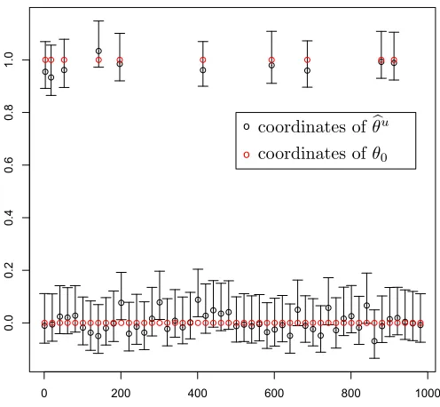
Figure 1: 95% confidence intervals for one realization of configuration (n, p, s0, b) = (1000,600,10,1). For clarity, we plot the confidence intervals for only 100 of the 1000 parameters. The true parametersθ0,i are in red and the coordinates of the debiased estimatorθbu are in black.
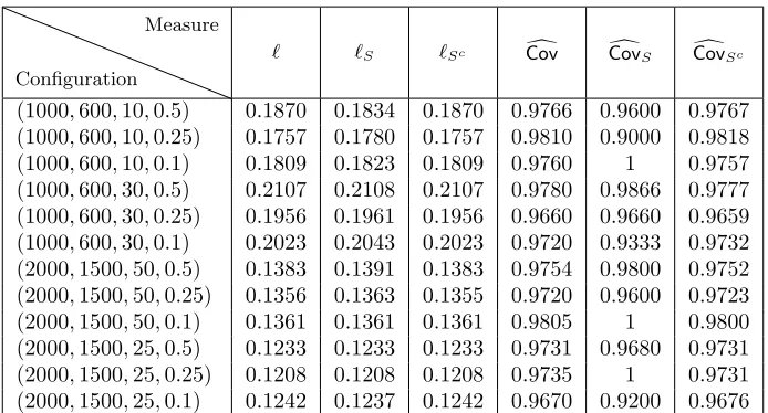
where bP denotes the empirical probability computed based on the 20 realizations for each configuration. The results are reported in Table 1. In Figure 1, we plot the constructed 95%-confidence intervals for one realization of configuration (n, p, s0, b) = (1000,600,10,1). For sake of clarity, we plot the confidence intervals for only 100 of the 1000 parameters.
False positive rates and statistical powers. Table 2 summarizes the false positive
rates and the statistical powers achieved by our proposed method, the multisample-splitting method (Meinshausen et al., 2009), and the ridge-type projection estimator (B¨uhlmann, 2013) for several configurations. The results are obtained by taking average over 20 indepen-dent realizations of measurement errors for each configuration. As we see the multisample-splitting achieves false positive rate 0 on all of the configurations considered here, making no type I error. However, the true positive rate is always smaller than that of our proposed method. By contrast, our method achieves false positive rate close to the pre-assigned significance level α = 0.05 and obtains much higher true positive rate. Similar to the multisample-splitting, the ridge-type projection estimator is conservative and achieves false positive rate smaller than α. This, however, comes at the cost of a smaller true positive rate than our method. It is worth noting that an ideal testing procedure should allow to control the level of statistical significanceα, and obtain the maximum true positive rate at that level.
Configuration
Measure
` `S `Sc Covd CovdS CovdSc
(1000,600,10,0.5) 0.1870 0.1834 0.1870 0.9766 0.9600 0.9767 (1000,600,10,0.25) 0.1757 0.1780 0.1757 0.9810 0.9000 0.9818 (1000,600,10,0.1) 0.1809 0.1823 0.1809 0.9760 1 0.9757 (1000,600,30,0.5) 0.2107 0.2108 0.2107 0.9780 0.9866 0.9777 (1000,600,30,0.25) 0.1956 0.1961 0.1956 0.9660 0.9660 0.9659 (1000,600,30,0.1) 0.2023 0.2043 0.2023 0.9720 0.9333 0.9732 (2000,1500,50,0.5) 0.1383 0.1391 0.1383 0.9754 0.9800 0.9752 (2000,1500,50,0.25) 0.1356 0.1363 0.1355 0.9720 0.9600 0.9723 (2000,1500,50,0.1) 0.1361 0.1361 0.1361 0.9805 1 0.9800 (2000,1500,25,0.5) 0.1233 0.1233 0.1233 0.9731 0.9680 0.9731 (2000,1500,25,0.25) 0.1208 0.1208 0.1208 0.9735 1 0.9731 (2000,1500,25,0.1) 0.1242 0.1237 0.1242 0.9670 0.9200 0.9676
Table 1: Simulation results for the synthetic data described in Section 5.1. The results corresponds to 95% confidence intervals.
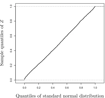
LetZ = (zi)pi=1denote the vector withzi ≡ √
n(θbui−θ0,i)/ b
σ
q
[MΣbMT]i,i. Figure 2 shows the sample quantiles of Z versus the quantiles of the standard normal distribution for one realization of the configuration (n, p, s0, b) = (1000,600,10,1). The scattered points are close to the line with unit slope and zero intercept. This confirms the result of Theorem 13 regarding the Gaussianity of the entries zi.
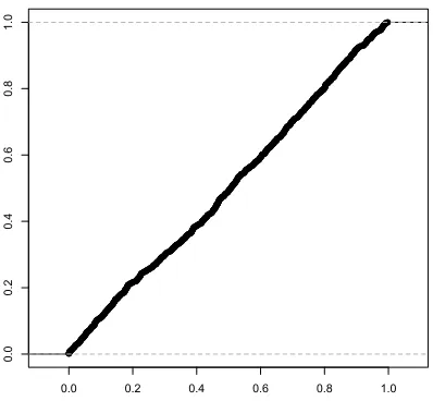
For the same problem, in Figure 3 we plot the empirical CDF of the computedp-values restricted to the variables outside the support. Clearly, the p-values for these entries are uniformly distributed as expected.
5.2 Real Data
As a real data example, we consider a high-throughput genomic data set concerning ri-boflavin (vitaminB2) production rate. This data set is made publicly available by B¨uhlmann et al. (2014) and contains n = 71 samples and p = 4,088 covariates corresponding to
p = 4,088 genes. For each sample, there is a real-valued response variable indicating the logarithm of the riboflavin production rate along with the logarithm of the expression level of the p= 4,088 genes as the covariates.
Following B¨uhlmann et al. (2014), we model the riboflavin production rate as a linear model with p = 4,088 covariates and n = 71 samples, as in Equation (1). We use the R packageglmnet(Friedman et al., 2010) to fit the LASSO estimator. Similar to the previous section, we use the regularization parameter λ= 4bσ
p
(2 logp)/n, where bσ is given by the scaled LASSO as per equation (31) with λe = 10
p
(2 logp)/n. This leads to the choice
-3 -2 -1 0 1 2 3
-2
0
2
4
Quantiles of standard normal distribution
Sample
quan
tiles
of
Z
Figure 2: Q-Q plot ofZ for one realization of configuration (n, p, s0, b) = (1000,600,10,1).
0.0 0.2 0.4 0.6 0.8 1.0
0.0
0.2
0.4
0.6
0.8
1.0
Our method Multisample-splitting Ridge projection estimator
Configuration FP TP FP TP FP TP
(1000,600,10,0.5) 0.0452 1 0 1 0.0284 0.8531 (1000,600,10,0.25) 0.0393 1 0 0.4 0.02691 0.7506 (1000,600,10,0.1) 0.0383 0.8 0 0 0.2638 0.6523 (1000,600,30,0.5) 0.0433 1 0 1 0.0263 0.8700 (1000,600,30,0.25) 0.0525 1 0 0.4 0.2844 0.8403 (1000,600,30,0.1) 0.0402 0.7330 0 0 0.2238 0.6180 (2000,1500,50,0.5) 0.0421 1 0 1 0.0301 0.9013 (2000,1500,50,0.25) 0.0415 1 0 1 0.0292 0.8835 (2000,1500,50,0.1) 0.0384 0.9400 0 0 0.02655 0.7603 (2000,1500,25,0.5) 0.0509 1 0 1 0.0361 0.9101 (2000,1500,25,0.25) 0.0481 1 0 1 0.3470 0.8904 (2000,1500,25,0.1) 0.0551 1 0 0.16 0.0401 0.8203
Table 2: Simulation results for the synthetic data described in Section 5.1. The false positive rates (FP) and the true positive rates (TP) are computed at significance level
α= 0.05.
We use Equation (35) to construct p-values for different genes. Adjusting FWER to 5% significance level, we find two significant genes, namely genes YXLD-at and YXLE-at. By contrast, the multisample-splitting method proposed in Meinshausen et al. (2009) finds only the geneYXLD-atat the FWER-adjusted 5% significance level. Also the Ridge-type projec-tion estimator, proposed in B¨uhlmann (2013), returns no significance gene. (See B¨uhlmann et al. 2014 for further discussion on these methods.) This indicates that these methods are more conservative and produce typically larger p-values.
In Figure 4 we plot the empirical CDF of the computed p-values for riboflavin example. Clearly the plot confirms that thep-values are distributed according to uniform distribution.
6. Proofs
This section is devoted to the proofs of theorems and main lemmas.
6.1 Proof of Theorem 6
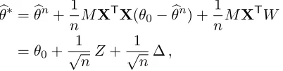
Substituting Y =Xθ0+W in the definition (7), we get
b
θ∗ =θbn+ 1
nMX
TX(θ
0−bθn) + 1
nMX
TW
=θ0+ 1 √
nZ+
1 √
n∆,
(62)
0.0 0.2 0.4 0.6 0.8 1.0
0.0
0.2
0.4
0.6
0.8
1.0
Quantiles of standard normal distribution
Sample
quan
tiles
of
Z
Figure 4: Empirical CDF of the computedp-values for riboflavin example. Clearly the plot confirms that thep-values are distributed according to uniform distribution.
We are left with the task of proving the bound (11) on ∆. Note that by definition (4), we have
k∆k∞≤
√
n|MΣb−I|∞kbθn−θ0k1= √
n µ∗kbθn−θ0k1. (63) By B¨uhlmann and van de Geer (2011, Theorem 6.1, Lemma 6.2), we have, for any λ ≥ 4σp2Klog(pet2/2
)/n
P
kbθn−θ0k1 ≥ 4λs0
φ2 0
≤2e−t2/2. (64)
(More precisely, we consider the trivial generalization of B¨uhlmann and van de Geer 2011, Lemma 6.2 to the case (XTX/n)ii≤K, instead of (XTX/n)ii= 1 for all i∈[p].)
Substituting Equation (63) in the last bound, we get
P
k∆k∞≥
4λµ∗s0 √
n φ2
0
≤2e−t2/2. (65)
Finally, the claim follows by selecting tso that et2/2 =pc0.
6.2 Proof of Theorem 7.(a)
Note that the eventEn requires two conditions. Hence, its complement is given by
En(φ0, s0, K)c=B1,n(φ0, s0)∪ B2,n(K), (66) B1,n(φ0, s0)≡
n
X∈Rn×p : min
S:|S|≤s0
φ(Σb, S)< φ0, Σ = (Xb TX/n) o
, (67)
B2,n(K)≡ n
X∈Rn×p : max
i∈[p] b
Σi,i> K, Σ = (Xb TX/n) o
We will bound separately the probability of B1,n and the probability of B2,n. The claim of Theorem 7.(a) follows by union bound.
6.2.1 Controlling B1,n(φ0, s0)
It is also useful to recall the notion of restricted eigenvalue, introduced by Bickel, Ritov and Tsybakov (Bickel et al., 2009).
Definition 22 Given a symmetric matrix Q ∈ Rp×p an integer s
0 ≥ 1, and L > 0, the
restricted eigenvalue of Q is defined as
φ2RE(Q, s0, L)≡ min S⊆[p],|S|≤s0
min θ∈Rp
nhθ, Q θi kθSk22
: θ∈Rp, kθSck1≤LkθSk1 o
. (69)
Rudelson and Shuheng (2013) prove that, if the population covariance satisfies the re-stricted eigenvalue condition, then the sample covariance satisfies it as well, with high probability. More precisely, by Rudelson and Shuheng (2013, Theorem 6) we have
P
φRE(Σb, s0,3)≥ 1
2φRE(Σ, s0,9)
≥1−2e−n/(4c∗κ4), (70) for somec∗ ≤2000,m≡6×10⁴s0Cmax2 /φ2RE(Σ, s0,9), and everyn≥4c∗mκ4log(120ep/m).
Note thatφRE(Σ, s0,9)≥σmin(Σ)1/2 ≥ √
Cmin, and by Cauchy-Schwartz, min
S:|S|≤s0
φ(bΣ, S)≥φRE(Σb, s0,3).
With the definitions in the statement (cf. Equation 13), we therefore have
P
min S:|S|≤s0
φ(bΣ, S)≥ 1 2
p
Cmin
≥1−2e−c1n. (71)
Equivalently, P(B1,n(φ0, s0))≤2e−c1n.
6.2.2 Controlling B2,n(K) By definition
b
Σii−1 = 1
n
n X
`=1
(hX`, eii2−1) = 1
n
n X
`=1
u`, . (72)
Note that u` are independent centered random variables. Further, (recalling that, for any random variables U, V, kU +Vkψ1 ≤ kUkψ1 +kVkψ1, and kU2kψ1 ≤ 2kUk2
ψ2) they are
subexponential with subexponential norm
ku`kψ1 ≤2khX`, eii
2k
ψ1 ≤4khX`, eiik
2 ψ1
≤4khΣ−1/2X`,Σ1/2eiik2ψ1
By Bernstein-type inequality for centered subexponential random variables, cf. Vershynin (2012), we get
P n1
n
n X
`=1
u` ≥ε
o
≤2 exph−n 6min
( ε
4eκ2) 2, ε
4eκ2 i
. (73)
Hence, for allεsuch thatε/(eκ2)∈[p(48 logp)/n,4],
P
max i∈[p]
b
Σii≥1 +ε
≤2pexp
− nε 2 24e2κ4
≤2e−c1n, (74)
which impliesP(X∈ B2,n(K))≤2e−c1nfor allK−1≥20κ2 p
(logp)/n≥p(48e2κ4logp)/n. 6.3 Proof of Theorem 7.(b)
Obviously, we have
µmin(X)≤
Σ−1Σb−I
, (75)
and hence the statement follows immediately from the following estimate.
Lemma 23 Consider a random design matrix X ∈ Rp×p, with i.i.d. rows having mean
zero and population covariance Σ. Assume that
(i) We haveσmin(Σ)≥Cmin>0, andσmax(Σ)≤Cmax<∞. (ii) The rows ofXΣ−1/2 are sub-Gaussian withκ=kΣ−1/2X
1kψ2.
LetΣ = (Xb TX)/nbe the empirical covariance. Then, for any constantC >0, the following
holds true.
P
Σ
−1 b Σ−I
∞≥a
r logp
n
≤2p−c2, (76)
with c2= (a2Cmin)/(24e2κ4Cmax)−2.
Proof [Proof of Lemma 23] The proof is based on Bernstein-type inequality for sub-exponential random variables (Vershynin, 2012). Let ˜X` = Σ−1/2X`, for ` ∈ [n], and write
Z ≡Σ−1Σb−I = 1
n
n X
`=1 n
Σ−1X`X`T−I o
= 1
n
n X
`=1 n
Σ−1/2X˜`X˜`TΣ1/2−I o
.
Fixi, j∈[p], and for`∈[n], letv`(ij) =hΣ−i,·1/2,X˜`ihΣ1j,/·2,X˜`i −δi,j, whereδi,j =1{i=j}.
No-tice thatE(v(`ij)) = 0, and thev (ij)
` are independent for`∈[n]. Also,Zi,j = (1/n) Pn
`=1v (ij) ` . By Vershynin (2012, Remark 5.18), we have
kv(`ij)kψ1 ≤2khΣi,−·1/2,X˜`ihΣ 1/2
Moreover, for any two random variablesX andY, we have
kXYkψ1 = sup
p≥1
p−1E(|XY|p)1/p ≤sup
p≥1
p−1E(|X|2p)1/2pE(|Y|2p)1/2p ≤2
sup q≥2
q−1/2E(|X|q)1/q sup
q≥2
q−1/2E(|Y|q)1/q
≤2kXkψ2kYkψ2.
Hence, by assumption (ii), we obtain
kv`(ij)kψ1 ≤2khΣ
−1/2
i,· ,X˜`ikψ2khΣ
1/2
j,· ,X˜`ikψ2
≤2kΣ−i,·1/2k2kΣj,1/·2k2κ2 ≤2pCmax/Cminκ2.
Letκ0= 2pCmax/Cminκ2. Applying Bernstein-type inequality for centered sub-exponential random variables (Vershynin, 2012), we get
P n1
n
n X
`=1
v`(ij)
≥ε
o
≤2 exph−n 6min
( ε
eκ0)
2, ε
eκ0
i
.
Choosingε=ap(logp)/n, and assuming n≥[a/(eκ0)]2logp, we arrive at
P
1
n
n X
`=1
v`(ij)
≥a
r logp
n
≤2p−a2/(6e2κ02).
The result follows by union bounding over all possible pairs i, j∈[p].
6.4 Proof of Theorem 8 Let
∆0≡16ac σ
Cmin
s0logp √
n (77)
be a shorthand for the bound on k∆k∞ appearing in Equation (17). Then we have
P
k∆k∞≥∆0
≤P
k∆k∞≥∆0 ∩ En( p
Cmin/2, s0,3/2)∩ Gn(a)
+P En( p
Cmin/2, s0,3/2)
+P Gnc(a)
≤P
k∆k∞≥∆0 ∩ En( p
Cmin/2, s0,3/2)∩ Gn(a)
+ 4e−c1n+ 2p−c2,