Author(s)
Mak, SHT; Best, NG; Rushton, L
Citation
International Journal of Biostatistics, 2015, v. 11 n. 1, p. 135-149
Issued Date
2015
URL
http://hdl.handle.net/10722/214691
Timothy Shin Heng Mak*, Nicky Best and Lesley Rushton
Robust Bayesian Sensitivity Analysis for Case
–
Control
Studies with Uncertain Exposure Misclassification
Probabilities
Abstract:Exposure misclassification in case–control studies leads to bias in odds ratio estimates. There has been considerable interest recently to account for misclassification in estimation so as to adjust for bias as well as more accurately quantify uncertainty. These methods require users to elicit suitable values or prior distributions for the misclassification probabilities. In the event where exposure misclassification is highly uncertain, these methods are of limited use, because the resulting posterior uncertainty intervals tend to be too wide to be informative. Posterior inference also becomes very dependent on the subjectively elicited prior distribution. In this paper, we propose an alternative“robust Bayesian”approach, where instead of eliciting prior distributions for the misclassification probabilities, a feasible region is given. The extrema of posterior inference within the region are sought using an inequality constrained optimization algorithm. This method enables sensitivity analyses to be conducted in a useful way as we do not need to restrict all of our unknown parameters to fixed values, but can instead consider ranges of values at a time.
Keywords:misclassification, robust Bayes, case–control study, Bayesian
DOI 10.1515/ijb-2013-0044
1 Introduction
Exposure misclassification is a common problem in case–control studies. When exposure misclassification is present, estimates of exposure prevalences and odds ratios are biased. Early references have pointed out that if the extent of misclassification is the same for both cases and controls and a dichotomous exposure is used, then bias is towards the null, and thep-value is not affected [4, 7], such that if a positive/negative relationship is demonstrated between exposure and disease, the evidence for the relationship being positive/negative is not affected by misclassification, under frequentist inference anyway. However, even if this is the case, estimates remain biased, and confidence intervals are inaccurate, and in Bayesian inference, the implication of bias towards the null is also not necessarily true [21]. Moreover, it has been argued that even small departures from the strict non-differential misclassification assumption does not warrant the“bias towards the null”implication [23], and so inference based on the misclassified exposure becomes even less reliable.
Assuming a binary (dichotomous) exposure, then true exposure prevalence (π) and misclassified exposure prevalence (p) are related through a simple formula:
p¼πsensþ ð1 πÞð1 specÞ ð1Þ
*Corresponding author: Timothy Shin Heng Mak,Centre for Genomic Sciences, University of Hong Kong, 5 Sassoon Road, Pokfulam, Hong Kong, E-mail: [email protected]
Nicky Best, Lesley Rushton,Department of Epidemiology and Biostatistics, Imperial College London, London, UK, E-mail: [email protected], [email protected]
wheresensis thesensitivityandspecthespecificityof the exposure measure and is defined as:
sens¼
Number of truly exposed people who
would have been categorized as exposed in the population
Total number of truly exposed people in the population
spec¼
Number of truly unexposed people who
would have been categorized as unexposed in the population
Total number of truly unexposed people in the population
Because of this simple relationship, it has been proposed in the literature [1, 7, 28, 30] that the misclassified exposure prevalence estimate can be corrected in order to estimate the true relative risk/odds ratio, and variance formulae for the adjusted estimate can be obtained using the delta method or maximum likelihood for large samples [14]. In the case of a binary exposure, the adjustment formula is simply the inverse of (1):
^
π¼ ^p1þspec
sensþspec1 ð2Þ
where ^pis an estimate ofpand^π theadjustedestimate ofπ. Adjustment formulae such as (2), however, assume that the misclassification probabilities sens and specare known. This, however, is almost never the case. Even in situations where these probabilities can be estimated from a validation study, estimates are subject to sampling error. In many situations, validation studies are not available, and estimates of
sens andspecwill have to depend entirely on intelligent guesses, if the adjustment formulae were to be used at all. Perhaps for this reason, even though exposure misclassification is widespread in epidemiology, adjustment for bias due to misclassification appears to be rarely applied.
Another problem with the adjustment formulae (such as (2)) is that sometimes the adjusted estimate for
π (i.e.^π) is undefined. For example, if a rare exposure is involved, with prevalence of exposurep¼0:01, then so long assens>0:01, any value ofspec<0:99 leads to an undefined estimate forπ, since according to (2),^πis either negative or greater than 1. This happens because althoughsensandspecare fixed (they are
populationvalues),p^is subject to sampling error and may lead to estimates that are incompatible with the population parameterssensandspec.
To a certain extent, the above problems can be overcome by adopting a Bayesian approach, as has been demonstrated by Gustafson, Le and Saskin [22], Gustafson [19], Chu, Gustafson and Le [6] and MacLehose and Gustafson [29]. In these authors’approach, prior distributions are given toπ1,π0, sens1,sens0,spec1,
spec0, where the subscript 1 refers to the case population and 0 the control population, and the posterior
distribution of the odds ratio ¼ ππ1ð10ð1ππ0Þ1Þis sought, through the model
Yi,BinðNi;piÞ; i¼0;1 ð3Þ
pi¼πisensiþ ð1πiÞð1speciÞ
whereYidenotes the number of exposed subjects andNithe total number of cases or controls. Estimation of
the posterior distribution can be derived through Markov chain Monte Carlo, which is easily implemented in software such as WinBUGS [27]. This approach does not make use of the estimate p^, and hence is not affected by possible incompatibility between ^pand sensand spec. There are, however, still a number of potential difficulties, such as:
1. It may not be immediately clear which parameterization we should adopt for the model. In the above-cited studies, prior distributions are given to the parametersπ1, π0,sens1,sens0,spec1,spec0. On the
other hand, Chu, Wang, Cole and Greenland [5] assigned prior distributions to π0 and
ðlogitπ1logitπ0Þ (instead of π0 and π1). Still, other vastly different parameterizations could have
also been used (e.g. [8, 16]). The choice of parameterization is especially unclear when there are no suitable estimates ofsens1,sens0,spec1,spec0 from validation studies.
2. If the extent of misclassification is great, the posterior distribution of the odds ratio becomes especially sensitive to the choice of prior and parameterization (to be demonstrated in Section 2). Moreover, accurate elicitation of prior distribution is made more difficult by the fact that it is often reasonable that prior distributions of the parameters are correlated [5, 6,9], as elicitation of correlation is difficult [11]. 3. Because inference from these analyses can depend so crucially on subjectivelyelicited probability distributions for the misclassification parameters, it is unsure what conclusions can be drawn by a reader who does not agree with the prior distributions used.
Because of the problems listed above, the goal of this paper is to present an alternative approach to analysing case–control studies subject to exposure misclassification, which is a type of robust Bayes analysis. Robust Bayes inference [2, 3] was originally introduced to examine the robustness of Bayesian estimates to departure from prior distributional assumptions. One type of robust Bayes analysis seeks the maximum and minimum possible inference from a class of prior distributions [12]. This type of analysis overcomes an important limitation in subjective Bayesian analysis, namely that it is rarely possible to specify auniqueprior distribution for a particular analysis. Although philosophically appealing, this type of analysis has not been widely applied in practice, probably because of computational difficulties. This paper aims to demonstrate its use in solving an epidemiological problem, as well as to show that this type of analysis is not computationally infeasible.
In the rest of this paper, we illustrate some of the deficiencies of the Bayesian approach in Section 2, with reference to the example of a case–control study of childhood leukaemia and electromagnetic fields (EMF) exposure. In Section 3, the approach of this paper is introduced. Section 4 and 5 give further extension of the method. Section 6 discusses the use of the method in sensitivity analyses. Concluding remarks are given in Section 7.
2 Deficiencies of the Bayesian approach in accounting for bias
due to exposure misclassification in case
–
control studies
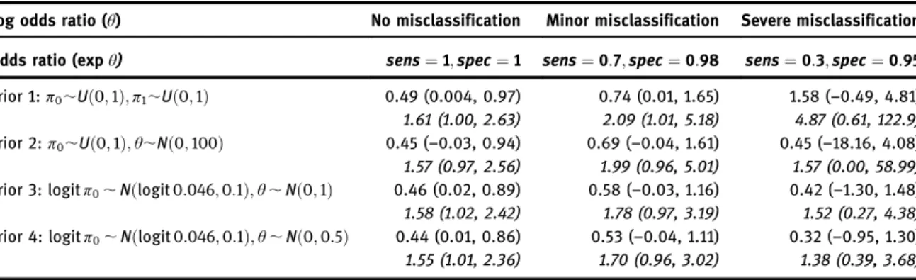
In this section, we consider how Bayesian inference in the presence of exposure misclassification can be very sensitive to the prior distribution used. First, consider the case–control study by Linet, Hatch, Kleinerman, Robison, Kaune, Friedman, Severson, Haines, Hartsock, Niwa, Wacholder and Tarone [26] on the risk of childhood leukaemia and exposure to high levels of EMF. EMF exposure was assessed by 24 h bedroom measurements at a convenient time (which can be up to a few years) after the diagnosis of leukaemia, where possible, and spot measurements around the residence where this was not possible. Controls were matched to the cases by sex and age and recruited by random-digitdialling. Out of 624 cases, 45 had EMF measurements >0:3μT (micro-Tesla). Among the 615 controls, 28 had measurements >0:3μT. This resulted in an odds ratio estimate of 1.63 comparing the risk of leukaemia in the >0:3μT group versus the <0:3μT group, with standard large sample 95% confidence interval (1.00, 2.65). Because the exposure measurement was performed in the residences of the children potentially several years after the etiologi-cally relevant period, severe misclassification of exposure is very possible. Bayesian inference for this dataset can be conducted using model (3). In Table 1, we compare the posterior median and 95% credible interval of the (log) odds ratio under three non-differential misclassification scenarios (no misclassification, minor misclassification and severe misclassification), using four different prior distributions. Results are derived using WinBUGS 1.4 [27].
Priors 1 and 2 are both weakly informative. Prior 1, in particular, was used by Gustafson et al. [22]. It has been argued that prior distributions should be given independently toπ0andθ, rather thanπ0andπ1[15],
where
This is the case for priors 2, 3 and 4. Prior 2 has nearly flat prior distribution for bothπ0andθ, whereas in
priors 3 and 4, the distribution for π0 is made to have mean equal to the mean ofp0¼Y0=N0¼0:046, the
observed prevalence of exposure among the controls, on the log-odds scale. Prior 3 differs from prior 4 in that for prior 3, the variance ofθis 1, while for prior 4 the variance is 0.5. The former corresponds to a 95% credible interval for the odds ratio ¼ (0.14, 7.1). The latter corresponds to a 95% credible interval of (0.25, 4.0).
It can be seen that posterior inference forθ, the log odds ratio, is similar using all four different prior distributions in the“no misclassification”and the“minor misclassification”scenario. However, the poster-ior inference under the“severe misclassification”scenario is very sensitive to the prior distributions given. The above results show that in the presence of severe exposure misclassification, the prior distribution of θ has a large impact on the posterior distribution. This is the case even if the misclassification probabilities sensi;speci are known. An intuitive explanation of this may be seen by considering the
variance ofπiin comparison to the variance ofpi(supposing fixedsensiandspeci):
Varπi¼Var pi1þspeci
sensiþspeci1
¼ VarðpiÞ
ðsensiþspeci1Þ2
ðcf eq:ð2ÞÞ ð4Þ
We see that variance of πi is the variance of pi divided byðsensiþspeci1Þ2 and is likely to be much
greater than the variance ofpiifsensiþspeciis close to 1. Becauseθ¼logitπ1logit0, the variance ofθis
also likely to be much larger than the variance of the log-observed odds ratio logitp1logitp0, if
sensiþspeciis close to 1. Thus we see that the data are“diluted”and the posterior distribution becomes
more influenced by the prior distribution.
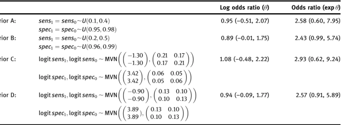
As another example, we examined the sensitivity of posterior inference to specification of the prior distribution for the misclassification probabilities (sens1;sens0;spec1;spec0). For this example, we fixed the
prior distribution forπ0andθat logitπ0,Nðlogit 0:046;0:1Þ;θ,Nð0;1Þ(prior 3). In Table 2, priors A and B
assume non-differential misclassification and consist of uniform priors given to sensandspec, though with different but largely overlapping ranges. Priors C and D assign bivariate Normal distributions to ðlogitsens1;logitsens0Þ andðlogitspec1;logitspec0Þ, with a correlation of 0.8. Means and variance of these
bivariate Normal distributions are chosen such that their 2.5% and 97.5%-ile match the limits of priors A and B. As can be seen, although the variation is not as great as those seen in the last column of Table 1, there are still considerable differences between the results. Thus, when presented with a Bayesian analysis of a case– control study with potentially severe misclassification, one set of results is rarely enough. We generally need to examine various situations to see how sensitive the results are to prior distributions used.
In view of these limitations, one may ask whether there is an alternative way to quantify our uncertainties over such Bayesian analysis. In the next section, we present the robust Bayesian method of this paper as one such alternative.
Table 1:Posterior median and 95% credible intervals forθunder different non-differential exposure misclassification scenarios and different prior distributions.
Log odds ratio (θ) No misclassification Minor misclassification Severe misclassification Odds ratio (expθ) sens¼1;spec¼1 sens¼0:7;spec¼0:98 sens¼0:3;spec¼0:95 Prior 1:π0,Uð0;1Þ;π1,Uð0;1Þ 0.49 (0.004, 0.97) 0.74 (0.01, 1.65) 1.58 (–0.49, 4.81) 1.61 (1.00, 2.63) 2.09 (1.01, 5.18) 4.87 (0.61, 122.9) Prior 2:π0,Uð0;1Þ;θ,Nð0;100Þ 0.45 (–0.03, 0.94) 0.69 (–0.04, 1.61) 0.45 (–18.16, 4.08) 1.57 (0.97, 2.56) 1.99 (0.96, 5.01) 1.57 (0.00, 58.99) Prior 3: logitπ0,Nðlogit0:046;0:1Þ;θ,Nð0;1Þ 0.46 (0.02, 0.89) 0.58 (–0.03, 1.16) 0.42 (–1.30, 1.48)
1.58 (1.02, 2.42) 1.78 (0.97, 3.19) 1.52 (0.27, 4.38) Prior 4: logitπ0,Nðlogit0:046;0:1Þ;θ,Nð0;0:5Þ 0.44 (0.01, 0.86) 0.53 (–0.04, 1.11) 0.32 (–0.95, 1.30)
3 A proposed method for robust Bayesian analysis for
case
–
control studies with potentially severe exposure
misclassification
Assume that our target parameter of interest isθ, given a suitable range of possible values forη, a set of nuisance parameters, the goal of the method of this paper is to find the feasible range of ^θðηÞ. In the exposure misclassification example, for example, η¼ fsens1;sens0;spec1;spec0;π0g. Here, we have
denoted by^θðηÞan estimate ofθ, givenη, such that the goal can be written as minimize=maximize^θðηÞoverηsubject toη2e
In this paper,^θðηÞrepresent certain percentile values of the posterior distribution ofθgivenηand the data. Thus, ifθ^ðηÞis the posterior median, then
½min
η2e^θðηÞ;maxη2e ^θðηÞ
defines the feasible range of the posterior medians ofθ.
A similar aim has been described by Vansteelandt, Goetghebeur, Kenward and Molenberghs [31], although these authors did not use a Bayesian estimate or credible interval for ^θðηÞ. In principle, the methods of this paper can be applied to other non-Bayesian estimators for ^θðηÞ. However, Bayesian estimators are used here in order that we may take advantage of the use of informative prior distributions, which can greatly aid the extraction of meaningful information from data with severe misclassification, as we have seen in Section 2.
Furthermore, by seeking½min
η2e^θðηÞ;maxη2e ^θðηÞ, we provide bounds to the set of posterior median/credible
intervals for the set of priors forðθ;ηÞwhereθandηare independent and that the density ofηis 0 outside
e, and thus provides a means of carrying robust Bayes analysis (see Appendix A).
In the exposure misclassification problem considered here, ^θðηÞ is a posterior percentile of the log odds ratioθ, which is the inverse function of the cumulative posterior distribution function of θ. Thus, denoting the cumulative distribution by FðθjX;ηÞ and its inverse by F1θjX;ηðpÞ for a percentile p, we have:
^
θðηÞ ¼Fθ1jX;ηðpÞ
Table 2:Posterior median and 95% credible intervals forθusing different prior distributions forsens1,sens0,spec1,spec0. Prior
distribution forπ0andθis the same as prior 3 of Table 1.
Log odds ratio (θ) Odds ratio (expθ) Prior A: sens1¼sens0,Uð0:1;0:4Þ 0.95 (–0.51, 2.07) 2.58 (0.60, 7.95)
spec1¼spec0,Uð0:95;0:98Þ
Prior B: sens1¼sens0,Uð0:2;0:5Þ 0.89 (–0.01, 1.75) 2.43 (0.99, 5.74)
spec1¼spec0,Uð0:96;0:99Þ
Prior C: logitsens1;logitsens0,MVN
1:30 1:30 ; 00::2117 00::1721 1.08 (–0.48, 2.22) 2.93 (0.62, 9.24) logitspec1;logitspec0,MVN
3:42 3:42 ; 00::0605 00::0605
Prior D: logitsens1;logitsens0,MVN 00:90
:90
;00::1013 00::1013
0.94 (–0.09, 1.77) 2.57 (0.91, 5.89) logitspec1;logitspec0,MVN
3:89 3:89Þ; 0:13 0:10 0:10 0:13
FðθjX;ηÞ ¼ ðθ 1 pðθjX;ηÞdθ pðθjX;ηÞ ¼LikðXjθ;ηÞpðθjηÞ pðXjηÞ LikðXjθ;ηÞ ¼ N1 Y1 N0 Y0 pY1 1 ð1p1ÞN1Y1p0Y0ð1p0ÞN0Y0
pi¼πisensiþ ð1πiÞð1speciÞ; i¼0;1
logitπ1¼logitπ0þθ
whereXdenote the data:X¼ fY1;Y0;N1;N0g.
It can be seen that as a function ofθ, the likelihood LikðXjθ;ηÞonly depends onpY1
1 ð1p1ÞN1Y1, and
pY1
1 ð1p1ÞN1Y1 only depends onsens1,spec1 and π0, and not onsens0 andspec0. Thus, sens0 andspec0
cannot affect the posterior percentile functionθ^ðηÞ. Indeed, givenπ0, the likelihood does not even depend
onY0 andN0. We are therefore considering a probabilistic modelling of the case datafY1;N1gonly. This
may appear a very unusual way of analysing case–control data, but it has been suggested in Zelen and Parker [32] that in a case–control study, we may havea prioriinformation over the prevalence of exposure among the controls, if the controls are representative of the general population, and thus control data are not always necessary. In the presence of severe misclassification, the control data can tell us very little about the true exposure prevalence due to data dilution as discussed above, anda prioriinformation, such as the degree to which the prevalence of misclassified exposure differs from the prevalence of true exposure, can be as important or more important than the control data.
As an example, consider the control data of the above example, where we haveY0¼28;N0¼615.
Assuming an uninformative prior distribution of π0,Uð0;1Þ and supposing sens0¼0:3;spec0¼0:95
(severe misclassification), the posterior distribution of π0 has median and 95% credible interval 0.02
(0.0008, 0.08), while those for p0 is 0.055 (0.050, 0.070). Thus, the control data itself tells us very
little about the prevalence π0 (even though it gives us considerable information for the misclassified
prevalencep0).
As the information concerningπ0given by the data is limited, it is sensible to seek alternative sources
of information. One potential source of information can be gained by considering the measurement error model that relates the true exposure to the observed exposure. For example, assuming a classical measurement error model, the true exposure ought to have lower prevalence than the observed preva-lence. This can be seen by writing the observed EMF exposure levels (Z) as their true EMF levels (ζ) plus an error term ("):
Z¼ζþ"
where "is typically 0 centred, and "is independent of ζ. Our observed prevalence estimate (p¼Y=N) estimatesPrðZ>cÞ, and our true prevalence isPrðζ>cÞ, where c denotes a certain threshold, 0.3μT in this particular case. If ζ and " were both Normal, and " has 0 mean, then PrðZ>cÞ will always be greater than Prðζ>cÞ if Prðζ>cÞ<0:5. Since 0.3 μT is quite a high threshold for exposure, Prðζ>cÞ 0:5, and hence we would expect the observed prevalence to be greater than the true prevalence. Given that the 95% confidence intervals for p0 is (0.03, 0.065), let us tentatively assume
that a reasonable range for π0 is
3.1 Finding
min
b
θ
η2e
ð Þ
η
;
max
η2eb
θ η
ð Þ
To conduct the robust Bayesian analysis, we need to further specify feasible ranges for the parameterssens1
andspec1. As the misclassification is potentially severe, let us assume:
0:1sens10:5 ð6Þ
0:95spec11 ð7Þ
Equation (6)indicates that sensitivity is unlikely to be high.1This is because of the nature of the exposure assessment. For a rare exposure, however, it is often feasible to have a fairly tight bound on the specificity, such as (7). This is because if we believe that classification is better than chance, thenspec1>1p1.2 If
misclassification is non-differential, then spec1>1p0. Given that the 95% confidence interval for p0 is
(0.03, 0.065), it seems reasonable thatspec1has a lower bound of 0.95.
For the analysis, let us also assume at this stage that the prior distribution ofθis
θ,Nð0;0:5Þ although this can be relaxed later.
Our aim is to find
½min^θðπ0;sens1;spec1Þ;max^θðπ0;sens1;spec1Þ
subject to constraints (6)–(7) where ^θðπ0;sens1;spec1Þ denote the posterior median of θ given
ðπ0;sens1;spec1Þ. Since
θ¼logitπ1logitπ0
for^θþ¼max^θðπ0;sens1;spec1Þ, we want logitπ1 to be as positive as possible, while logitπ0 should be as
negative as possible. We note also that @π @sens¼ 1specp ðsensþspec1Þ2 >0 ifspec<1p ¼0 ifspec¼1p <0 ifspec>1p : 8 < : ð8Þ and @π @spec¼ sensp ðsensþspec1Þ2 >0 ifsens>p ¼0 ifsens¼p <0 ifsens<p 8 < : ð9Þ
ifsensþspecÞ1. Moreover, when sensþspec>1, senspand spec1p. Therefore for^θþ, we would expectsens1to be found at its minimum,spec1at its maximum andπ0at its minimum, and the reverse for
^
θ¼min^θðπ
0;sens1;spec1Þ. This implies that½^θ;^θþshould be
½^θðπ0¼0:05;sens1¼0:5;spec1¼0:95Þ;θ^ðπ0¼0:01;sens1¼0:1;spec1¼1Þ ¼ ½0:09;4:47
Of course, the above does not give us a proof that½^θ;^θþ ¼ ½0:09;4:47since the relationship between
^
θðπ0;sens1;spec1Þ and ðπ0;sens1;spec1Þ is much more complicated than that between θ and
1 If we assume the true exposure and the observed exposure levels follow a bivariate Normal distribution with equal mean, with the observed exposure levels having a standard deviation that is 1.2 times that of the true exposure, and correlation in the region of 0.3–0.7, then for an exposure classification defined by the top 5% of underlying exposure, the sensitivity is in the region of 0.1– 0.5. The range of correlation (0.3–0.7) comes from a study which estimatedr2 between bedroom measurements and
personal monitoring [10].
2This can be seen by rearranging (1) as spec¼1pþπðsensþspec1Þ. Because 0π1, when sensþspec>1,
ðπ0;sens1;spec1Þ. In order to give us more confidence that we have found our extremes, we may use a
search algorithm to identify½θ^;^θþ. For this purpose, we wrote a program in Matlab, which makes use of thefminconalgorithm in its Optimization Toolbox. The optimization took less than 1 s and confirmed that ðπ0¼0:05;sens1¼0:5;spec1¼0:95Þ and ðπ0¼0:01;sens1¼0:1;spec1¼0:95Þ are indeed local minimum
and maximum.
4 Allowing for uncertainty in the prior distribution of
θ
To facilitate exposition, in the previous section, we use the prior distribution of θ,Nð0;0:5Þ without explanation. This prior distribution places 95% weight in the odds ratio, i.e. expθ, being between 0.25 and 4.0. If the relationship between exposure to high levels of EMF and childhood leukaemia is unlikely to be greatly confounded by other factors (c.f.[24], such a prior distribution might be reasonable. It is also the prior distribution used by Greenland and Kheifets [18] in their meta-analysis of childhood leukaemia-EMF studies. However, it is understandable that not all readers may be happy with this prior. Some may find the prior too narrow, and others too wide. One advantage of using the method of this paper is that we can also specify a“range”of prior distribution. For example, it may be supposed that a“reasonable”range of prior variance for the Normal distribution may be from 0.3 to 0.7, such that we have:
θ,Nð0;σ2Þ
0:3σ20:7
Intuitively, the effect of having a prior distribution with a smaller variance is to shrink the estimates further towards zero. Therefore, we would expectσ2¼0:7 for both^θþand^θ, since previous calculations showed
that^θþis positive and^θis negative. Again a search algorithm may be used to confirm this. This is indeed the case for this example, and we have:
½^θ;^θþ ¼ ½0:11;4:67 ð10Þ
5 Imposing additional constraints in the parameters
sens1
,
spec1
and
π
0So far, we have only given bounds to the parameters pi0, sens1,spec1 and σ2. It may be asked whether
additional information concerning the sensitivity or specificity in the control population may help us further narrow our feasible region for^θ. Intuitively, giving bounds tosens0andspec0may help us narrow
the bounds onsens1andspec1since if misclassification is nearly non-differential,sens1;spec1should not be
too different from sens0;spec0. Furthermore, p0 is related tosens0, spec0 and π0 through (1). Therefore,
giving bounds top0can also potentially restrict our feasible region ofðπ0;sens1;spec1Þ.
In this section, we present a scheme that would enable us to determine whether a particular combina-tion ofπ0;sens1;spec1satisfies the constraints:
Given thatp^0¼28=615¼0:046 (95% confidence interval ¼ [0.03, 0.06]), let us assume
½p0p0 ½p0þ ð11Þ
sens
1sens0 ½sens1sens0þ ð12Þ
spec
for some"sensand"spec. In this section, we present a scheme that would enable us to determine whether a
particular combination ofπ0;sens1;spec1 satisfies constraints (11), (12), (13) also.
5.1 Determining if a set of (
π
0,
sens
1,
spec
1) falls within the feasible region
Denote the lower and upper bounds of a quantity x by ½x and ½xþ respectively, e.g. ½sens1sens1 ½sens1þ, ½spec1spec0spec1spec0 ½spec1spec0þ. To determine if a set of
ðπ0;sens1;spec1Þis feasible, we can consider the following:
1. Assuming all of the parameters are given feasible ranges, i.e.½xþ ½xfor all x, and assuming also 0<π0<1, check whether:
(a) Sðsens0Þ¼maxð½sens0;sens1 ½sens1sens0þÞ
>minð½sens0þ;sens1 ½sens1sens0Þ ¼Sðsens0Þþ
(b) Sðspec0Þ¼maxð½spec0;spec1 ½spec1spec0þÞ
>minð½spec0þ;spec1 ½spec1spec0Þ ¼Sðspec0Þþ
(c) Sðp0Þ¼ ½p0>½p0þ¼Sðp0Þþ
Evidently, if any of (a), (b) or (c) is true, the set ofðπ0;sens1;spec1Þis outside the feasible region, as it is
not possible to find values of sens0;spec0;sens1sens0;spec1spec0;p0;p0π0 that satisfy the
constraints.
2. If all of 1(a), 1(b), 1(c) are untrue, then we further test for feasibility by considering whether: max ðSðp0Þ ð1π 0Þð1Sðspec0ÞÞÞ=π0; Sðsens0Þ > min ðSðp0Þ þ ð1π 0Þð1Sðspec0ÞþÞÞ=π0; Sðsens0Þþ ! ð14Þ
If this is true thenðπ0;sens1;spec1Þis not feasible. If it is untrue, then it is feasible. This comes from the
fact thatsens0,spec0,π0andp0are related by identity (1). Equation (14) is derived by considering the
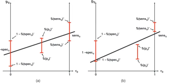
maximum and minimum ofsens0implied by constraints given tospec0andp0as well as the location of π0,sens1andspec1. The rationale behind the scheme can be seen by considering Figure 1. It can be seen
π0 p0 0 1 (a) (b) 1 –spec0 1 –spec0 S(p0) – S(p0)– S(p0)+ S(p0)+ 1 – S(spec0)+ 1 – S(spec0) + 1 – S(spec0) – 1 – S(spec 0) – S(sens0) – S(sens0) – S(sens0) + S(sens 0) + π0 p0 0 1 sens0 sens0
Figure 1:(a) A situation where the set ofðπ0;sens1;spec1Þis feasible as it is possible to draw a line through intervals defined by
½1Sðspec0Þþ;1Sðspec0Þ,½Sðπ0Þ;Sðπ0Þþand½Sðsens1Þ;Sðsens1Þþis shown. (b) A situation where it is not possible to
that in order that a ðπ0;sens1;spec1Þ be feasible, we must be able to draw a straight line through
½Sðp0Þ; Sðp0Þþ, ½Sðsens0Þ; Sðsens0Þþ and ½1Sðspec0Þþ; 1Sðspec0Þ. (This is because
p0¼π0 sens0þ ð1π0Þð1spec0Þ represents a linear relationship betweenp0and π0.) The range of
½Sðp0Þ; Sðp0Þþ,½Sðsens0Þ; Sðsens0Þþand½1Sðspec0Þþ; 1Sðspec0Þis in turn determined by the
position ofðsens1;spec1Þas well asπ0.
5.2 Finding
min
b
θ
η2e
ð Þ
η
;
max
η2eb
θ η
ð Þ
with additional constraints
Now assume we have the following constraints:
0:01π00:05 ð15Þ 0:1sens00:5 ð16Þ 0:25sens10:4 ð17Þ 0:95spec01 ð18Þ 0:95spec11 ð19Þ 0:03p00:065 ð20Þ 0:05sens1sens00:05 ð21Þ 0:02spec1spec00:02 ð22Þ 0:3σ20:7 ð23Þ
The presence of constraints such as (15)–(22) makes it difficult to use simple relationships such as (8) and (9) to locate the extremes of^θ. For this, an optimization algorithm becomes more useful. Still, it should be borne in mind that a surface such as^θðπ0;sens1;spec1Þis not necessarily convex, and multiple local optima
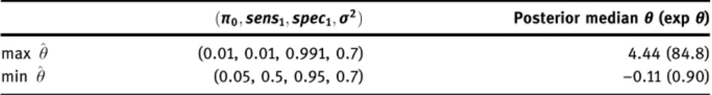
may exist. For this reason, it is necessary to repeat the optimization a number of times from different starting points in order to adequately explore the parameter space. For this particular example, we repeated the optimization 10 times (using Matlab’s fmincon as before) with the locations of the extrema given in Table 3.
Compared to the previous results (10), we see that the lower bound of–0.11 remained unchanged but the upper bound is shrunk towards 0. Thus, the effect of constraints (15)–(22) is to limit the upper extreme of^θ. The location of min^θis not limited by the additional constraints imposed in (15)–(22), although the location of max^θ is. The active constraints at max^θM and max^θU are (20), (21) and (22). These can be derived as results from the optimization.
Table 3:Location of ðπ0;sens1;spec1;σ2Þat the maximum and minimum posterior median ofθ
given the constraints of (15)–(23).
ðπ0;sens1;spec1;σ2Þ Posterior medianθ(expθ)
max^θ (0.01, 0.01, 0.991, 0.7) 4.44 (84.8)
6 The use of the method as a tool for sensitivity analysis
As noted in the introduction and Section 2 of this paper, Bayesian, probabilistic strategies for adjustment of exposure misclassification might suffice in the scenario where misclassification is not too serious, where the data are not too“diluted”. In the situation where exposure misclassification is potentially serious, not only does it become more difficult to elicit prior distributions for the parameters, but the dilution of the data means that it is unlikely that the data can tell us much about the direction ofθ. This is when the method of this paper is most useful. For example, we might ask, what values dosens1,sens0,spec1,spec0have to take
in order that we may have evidence of a positive relationship between EMF and childhood leukaemia, or how does departure from the assumption of non-differential misclassification affect inference? These questions can be answered by using the method of this paper.
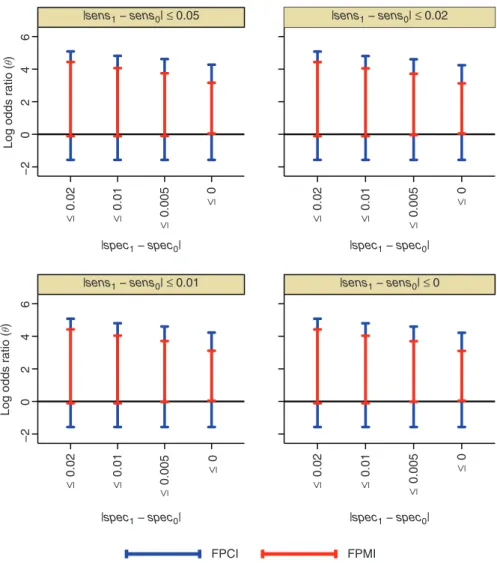
Before we discuss further, it will be useful to introduce the following terminology. Denoting by^θMðηÞthe posterior median ofθgivenηand^θLðηÞthe posterior 2.5%-ile and^θUðηÞthe posterior 97.5%-ile, let us define the
Feasible posterior median intervalðFPMIÞ ¼ ½min^θM;max^θM Feasible posterior credible intervalðFPCIÞ ¼ ½min^θL;max^θU
In Figure 2, we can examine how departures from non-differential misclassification affect the FPMI and FPCI. Here, we see that while departures from non-differential specificity increases the FPMI and FPCI,
−2
0
2
4
6
Log odds ratio (
θ
)
Log odds ratio (
θ ) ≤ 0.02 ≤ 0.01 ≤ 0.005 ≤ 0 |sens1 − sens0| ≤ 0.05 ≤ 0.02 ≤ 0.01 ≤ 0.005 ≤ 0 −2 0 2 4 6 ≤ 0.02 ≤ 0.01 ≤ 0.005 ≤ 0 ≤ 0.02 ≤ 0.01 ≤ 0.005 ≤ 0 FPCI FPMI |sens1 − sens0| ≤ 0.02
|sens1 − sens0| ≤ 0.01 |sens1 − sens0| ≤ 0
|spec1 − spec0|
|spec1 − spec0|
|spec1 − spec0| |spec1 − spec0|
Figure 2: Sensitivity analyses showing how FPMI and FPCI vary with departures from non-differential misclassification, assuming all other constraints hold.
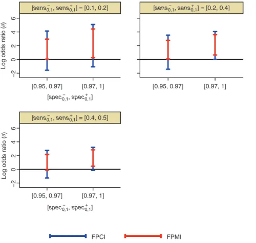
departures from non-differentialsensitivitydid not affect the intervals very much. In Figure 3, we can look at how restricting the ranges ofsens1;sens0;spec1;spec0affect the intervals. It can be seen that ifspec1and
spec0 were greater than 0.97, then there is greater evidence for a positive relationship between EMF and
childhood leukaemia. Assens0andsens1 increase, the width of the FPMI and FPCI decreases. We also see
that when ðspec1;spec0Þ are >0:97, andðsens1;sens0Þare between 0.2 and 0.4, the FPCI just includes 0.
Further increase inðsens1;sens0Þdoes not lead to the FPCI being further away from 0.
Finally we may also look at how π0 affect the FPMI and FPCI. In Figure 4, we can see that as π0
increases, the upper limit of the FPMI and FPCI become lower, but the lower limit remains nearly the same.
−2 0 2 4 6 [0.95, 0.97] [0.97, 1] [0.95, 0.97] [0.97, 1] −2 0 2 4 6 [0.95, 0.97] [0.97, 1] FPCI FPMI
Log odds ratio (
θ
)
Log odds ratio (
θ ) [sens0,1, sens0,1] = [0.1, 0.2] − + [sens0,1, sens0,1] = [0.2, 0.4] − + [sens0,1, sens0,1] = [0.4, 0.5] − + [spec0,1− , spec0,1+ ] [spec0,1, spec0,1] − +
Figure 3:Sensitivity analyses showing how FPMI and FPCI vary with changes in the feasible range ofsens1,sens0,spec1and
spec0, assuming all other constraints hold.
−2
0
2
4
6
Log odds ratio (
θ
)
[0.01, 0.02] [0.02, 0.03] [0.03, 0.04] [0.04, 0.05] [p0− , p0+]
FPCI FPMI
Figure 4:Sensitivity analyses showing how FPMI and FPCI vary with changes in the feasible range ofπ0, assuming all other
7 Discussion
In this paper, we have introduced a new method for carrying out sensitivity analysis in case–control studies subject to exposure misclassification bias. In traditional Bayesian analysis, in the presence of severe misclassification, results are very sensitive to the prior distributions given, and different investigators may have different prior distributions. A common way to deal with uncertainty in prior distributions is through the use of a hierarchical prior [13]. However, in specifying a hierarchical prior, one is still specifying aunique prior distribution. If one does not agree with the prior, one also cannot strictly agree with the posterior. The robust Bayesian approach of this paper offers an alternative. Instead of averaging out results from different prior distributions, we seek out the most extreme inference possible among a specified class of prior distributions. Readers can compare their own beliefs with the feasible region specified for the various parameters. If his/her belief falls within the feasible region, then his/her posterior inference will also fall within the FPMI/FPCI. If the feasible region is wide, however, inevitably the FPMI/FPCI will also be wide. In these situations, perhaps a better use of this method is in exploring what misclassi-fication probabilities are needed in order that the data may confer evidence in support of a positive or a negative association. As a tool for sensitivity analysis, the advantage of this approach is that one does not have to specify unique values for the uncertain parameters, but can instead specify ranges for the parameters.
A major contribution of this paper is its computational aspect. It is increasingly realized that data collected from observational studies cannot give unbiased estimates of epidemiological quantities of interest (e.g. [17, 20]), and that standard confidence intervals often underestimate the true uncertainty associated with estimates as they ignore bias. Therefore it has often been suggested that realistic models of epidemiologic data should take into account of uncertainty of bias by using models that integrate data with subjective “expert” knowledge [17, 20, 25]. Some have proposed that we seek out feasible region of inference given subjectively specified constraints for the unidentifiable parameters [31]. Application of these approaches, however, has been limited to simple scenarios, where such bounds can be computed analytically. In this paper, this is extended through the use of an optimization algorithm to situation where no such analytical solution exists. The method of this paper also paves the way for more general robust Bayesian inference, which has yet to become popular despite its philosophical integrity [2, 3]. The present paper shows that this type of inference is computationally feasible in a situation involving three unidentifi-able parameters, although the existence of multiple local minima/maxima remains a potential difficulty in the general adoption of this method. Because the computation is suitably fast in the example of this paper, optimization can be repeated at a large number of starting points to ensure that the failure to locate the global optima is unlikely. As the number of unidentifiable parameters increases, this may become more and more infeasible, and further research is needed to help us locate the global optima in those situations.
Appendix A: robust Bayes interpretation of FPMIs and FPCIs
In robust Bayes analysis, we seek to summarize the many possible posterior inferences arising from aclass
of prior distributions. Assumingθ andη are independent and supposing^θ is a posterior percentile ofθ, seeking the minimum and maximum of ^θ can be thought of as seeking the minimum and maximum posterior percentile among the class of prior distributions which have zero density outside the feasible region ofη. To see this, note that the posterior density ofθcan be written as:
pðθjXÞ ¼
ð
η
pðθ;ηjXÞdη
Denoting the cumulative distribution ofθgivenXbyFθjX:θ!p, which mapsθonto the percentilesp, we
FθjXðθÞ ¼ ðθ 1 ð η pðθ;ηjXÞdηdθ ¼ ðθ 1 ð η pðXjθ;ηÞpðθÞpðηÞpðXjηÞ
pðXjηÞpðXÞ dηdθ ðby Bayes’theoremÞ
¼ ð η ðθ 1 pðθjX;ηÞdθpðηjXÞdη ¼ ð η FθjX;ηðθÞpðηjXÞdη
Hence, we see that the cumulative distribution of θ given X is a weighted average of the cumulative distribution ofθgivenXandη. Now, if our prior distribution ofηbelongs to a class that has zero mass for values outside the feasible region ofη, denotede, i.e.:
pðηÞ ¼0 "η‚e
then
pðηjXÞ ¼0 "η‚e
and because averages cannot be greater than the maximum or less than the minimum, min
η2eFθjX;ηðθÞ FθjXðθÞ maxη2e FθjX;ηðθÞ
Now because our Bayesian estimates ^θ are percentile functions F1:p!θ, which is the inverse of the cumulative distribution function. Since the cumulative distribution function FðθÞ is necessarily a mono-tonically increasing function, we have:
min
η2e^θ¼minη2eF 1
θjX;ηðpÞ F1θjXðpÞ maxη2e Fθ1jX;ηðpÞ ¼maxη2e ^θ Thus, by finding min
η ^θand maxη ^θ, we give bounds toF
1
θjXðpÞ. Note that when we give bounds toFθ1jXðpÞ, we
are assuming that the prior distribution of θis the same as the prior distribution we use to calculate the bounds (i.e. Fθ1jXðpÞ andFθ1jX;ηðpÞshare the same prior distribution forθ). For this to be possible, the prior distribution ofθmust not depend onη.
References
1. Bashir S, Duffy S. The correction of risk estimates for measurement error. Ann Epidemiol 1997;7:154–64. 2. Berger J.The robust Bayesian viewpoint (with discussion). In:Kadane, J, editor. Robustness of Bayesian analysis.
Amsterdam: North-Holland, 1984:63–144.
3. Berger J. Robust Bayesian analysis: sensitivity to the prior. J Stat Plann Infer 1990;25:303–28. 4. Bross I. Misclassification in 2 by 2 tables. Biometrics 1954;10:478–86.
5. Chu H, Wang Z, Cole S, Greenland S. Sensitivity analysis of misclassification: a graphical and a Bayesian approach. Ann Epidemiol 2006;16:834–41.
6. Chu R, Gustafson P, Le N. Bayesian adjustment for exposure misclassification in case-control studies. Stat Med 2010;29: 994–1003.
7. Copeland K, Checkoway H, McMichael A, Holbrook R. Bias due to misclassification in the estimation of relative risk. Am J Epidemiol 1977;105:488–95.
8. Diamond E, Lilienfeld A. Effects of errors in classification and diagnosis in various types of epidemiological studies. Am J Public Health Nations Health 1962;52:1137–44.
9. Fox M, Lash T, Greenland S. A method to automate probabilistic sensitivity analyses of misclassified binary variables. Int J Epidemiol 2005;34:1370–6.
10. Friedman D, Hatch E, Tarone R, Kaune W, Kleinerman R, Wacholder S, et al.Childhood exposure to magnetic fields: residential area measurements compared to personal dosimetry. Epidemiology 1996;7:151–5.
11. Garthwaite P, Kadane J, O‘Hagan A. Statistical methods for eliciting probability distributions. J Am Stat Assoc 2005;100: 680–700.
12. Gelman A. The boxer, the wrestler, and the coin flip: a paradox of robust Bayesian inference and belief functions. Am Stat 2006;60:146–50.
13. Gelman A, Carlin J, Stern H, Rubin D. Bayesian data analysis. Boca Raton, FL: Chapman and Hall/CRC, 2004.
14. Greenland S. Variance-estimation for epidemiologic effect estimates under misclassification. Stat Mede 1988;7:745–57. 15. Greenland S. Sensitivity analysis, Monte Carlo risk analysis, and Bayesian uncertainty assessment. Risk Anal
2001;21:579–83.
16. Greenland S. Bayesian perspectives for epidemiologic research III. Bias analysis via missing-data methods. Int J Epidemiol 2009;38:1662–73.
17. Greenland S. Overthrowing the tyranny of null hypotheses hidden in causal diagrams. In:Dechter R, Geffner H, and Halpern J, editors. Heuristics, probabilities, and causality: a tribute to Judea Pearl. London: College Press, 2010:365–82. 18. Greenland S, Kheifets L. Leukemia attributable to residential magnetic fields: results from analyses allowing for study
biases. Risk Anal 2006;26:471–82.
19. Gustafson P. Measurement error and misclassification in statistics and epidemiology: impacts and Bayesian adjustments. Boca Raton, FL: Chapman and Hall, 2004.
20. Gustafson P. On model expansion, model contraction, identifiability and prior information: two illustrative scenarios involving mismeasured variables. Stat Sci 2005;20:111–29.
21. Gustafson P, Greenland S. Curious phenomena in Bayesian adjustment for exposure misclassification. Stat Med 2006;25:87–103.
22. Gustafson P, Le N, Saskin R. Case-control analysis with partial knowledge of exposure misclassification probabilities. Biometrics 2001;57:598–609.
23. Jurek A, Greenland S, Maldonado G. How far from non-differential does exposure or disease misclassification have to be to bias measures of association away from the null?Int JEpidemiol 2008;37:382–5.
24. Kheifets L, Shimkhada R. Childhood leukemia and EMF: review of the epidemiologic evidence. Bioelectromagnetics 2005;7: S51–9.
25. Lash T, Fox M, Fink A. Applying quantitative bias analysis to epidemiologic data. New York, NY: Springer, 2009. 26. Linet M, Hatch E, Kleinerman R, Robison L, Kaune W, Friedman D, et al.Residential exposure to magnetic fields and acute
lymphoblastic leukemia in children. N Engl J Med 1997;337:1–7.
27. Lunn D, Thomas A, Best N, Spiegelhalter D. WinBUGS – a Bayesian modelling framework: concepts, structure, and extensibility. Stat Comput 2000;10:325–37.
28. Lyles R. A note on estimating crude odds ratios in case-control studies with differentially misclassified exposure. Biometrics 2002;58:1034–6.
29. MacLehose R, Gustafson P. Is probabilistic bias analysis approximately Bayesian? Epidemiology 2012;23:151–8.
30. Morrissey M, Spiegelman D. Matrix methods for estimating odds ratios with misclassified exposure data: extensions and comparisons. Biometrics 1999;55:338–44.
31. Vansteelandt S, Goetghebeur E, Kenward M, Molenberghs G. Ignorance and uncertainty regions as inferential tools in a sensitivity analysis. Stat Sinica 2006;16:953–79.