Use of the Zero Norm with Linear Models and Kernel Methods (Kernel Machines Section)

(1)

Use of the Zero-Norm with Linear Models and Kernel Methods

Jason Weston [email protected]

Andr´e Elisseeff [email protected]

Bernhard Sch ¨olkopf [email protected]

BIOwulf Technologies, New York, USA; and

Max Planck Institute for Biological Cybernetics, 72076 T¨ubingen, Germany

Mike Tipping [email protected]

Microsoft Research, Cambridge, England

Editors: Leslie Pack Kaelbling

Abstract

We explore the use of the so-called zero-norm of the parameters of linear models in learning. Minimization of such a quantity has many uses in a machine learning context: for variable or feature selection, minimizing training error and ensuring sparsity in solutions. We derive a simple but practical method for achieving these goals and discuss its relationship to existing techniques of minimizing the zero-norm. The method boils down to implementing a simple modification of vanilla SVM, namely via an iterative multiplicative rescaling of the training data. Applications we investigate which aid our discussion include variable and feature selection on biological microarray data, and multicategory classification.

1. Introduction

In pattern recognition, many learning machines, given training data xi∈Rn,i=1,...,m with corre-sponding function values yi∈ {±1},i=1,...,m, make predictions g(x)about points x∈Rnof the form:

g(x) =sign(w·x+b)

(2)

Many generalizations of the original work of Boser, Guyon and Vapnik have been proposed. For instance, Bradley and Mangasarian (1998) describe the following general procedure is given to discriminate linearly separable data:

Problem 1 min

w kwk

p p

subject to : yi(w·xi+b)≥1

wherekwkp=

∑n j=1w

p j

1/p

is the`p-norm of w. When p=2, this procedure is the same as the optimal margin method. The generalization capabilities of such linear models have been studied by many researchers who have shown that, roughly speaking, minimizing the`p-norm of w is good for generalization. Such results hold for p≥1. In this paper, we study machines that are obtained as in Problem 1 in the extreme case when p→0, which we will call, in a slight abuse of terminology,1 the minimization of the zero-norm of w, the latter being defined as:

kwk0₀=card{wi|wi6=0} where card is set cardinality.

Pattern classification, especially in the context of regularization that enforces sparsity of the weight vector, is deeply connected to the problem of feature selection (Blum and Langley, 1997, pro-vide an introduction). In the feature selection problem one would like to select a subset of features while preserving or improving the discriminative ability of a classifier. In many supervised learning problems2 feature selection is important for a variety of reasons: generalization performance, run-ning time requirements, and constraints and interpretational issues imposed by the problem itself. Minimization of the zero-norm provides a natural way of directly addressing the feature selection and pattern classification objectives in a single optimization. However, this is achieved at the cost of having to solve a very difficult optimization problem which will not necessarily generalize well.

NP-Hardness For p=0, Amaldi and Kann (1998) show that Problem 1 is NP-Hard: it cannot even be approximated within 2log1−ε(n),∀ε>0 unless NP⊂DTIME(npoly log(n))where DTIME(x) is the class of deterministic algorithms ending in O(x) steps. It means that under rather general assumptions, there is no polynomial time algorithm that can approximate the value of the objective function at optimum N0within less than N0(2log1−ε(n))for allε>0. The minimization of Problem 1 is thus hopeless and very specific approximations need to be defined with well motivated discussions and experiments. This is the aim of this paper which presents a novel approximation in the context of Machine Learning. It turns out that in such a context a simple approximation of Problem 1 leads to a sufficiently small value of its objective function. The term ”sufficiently” is relative to the goal to be achieved. For instance, finding a small number of features so that there exists a linear model consistent with a training set does not require finding the smallest number of features. Most of the time reducing the size of the input space is done in order to get better generalization performance and not in order to have a compact representation of the inputs. So, sometimes finding the smallest

1. Note that for p<1,k.kpis not a norm, and that we consider herek.kpprather thank.kpso that the limit exists when

p→0.

(3)

subset of features is not desirable since it could lead to overfitting if the number of training points is small (for example consider if there are a very large number of noisy features and a very small training set size then one could pick a small number of the noisy features which appear highly correlated with the target, but do not generalize to new examples).

Applications The zero norm is directly related to some optimization problems in learning, for ex-ample in minimizing the number of training errors or finding minimal subsets, e.g., in vector quan-tization. In some applications we consider, however, the value of the objective functionkwk0₀is not exactly what has to be minimized. From a machine learning perspective, as we already mentioned, we are often more interested in the generalization performance. In feature selection problems one is often interested in parameterizing the problem to control the trade off between number of features used and training error (as well as regularizing appropriately). This has usually been solved in a two stage approach (feature selection, followed by minimizing error + regularization) but we show how, by using the zero norm with a constraint on the minimum number of features allowed, one can try to perform the error minimization and feature selection in one step. The latter is not re-stricted to only two-class models: we will derive a similar formulation as Problem 1 for multi-class discrimination. Feature selection for regression, for example, can also be cast into a mathematical problem similar to what we are studying here. The duality between feature selection and classifica-tion errors is known ((Amaldi and Kann, 1998)), and one can use the same technique to solve both problems. Minimizing the classification error on the training set or a trade-off between this error and the number of desired features is another application we deal with in this paper.

Previous work on minimizing the zero-norm Problem 1 already appeared in the literature: we mentioned the work of Amaldi and Kann who studied its computational complexity. In the Machine Learning community, the first work we are aware of concerning this problem is that of Bradley and Mangasarian. Bradley et al. (1995) and Bradley and Mangasarian (1998) propose an approximation method called FSV, which is used for variable selection and, later, by Fung et al. (2000), for finding sparse kernel expansions. It is based on an approximation of the step function:

kwk0₀=card{wi|wi6=0} ≈

∑

i

1−e−α|wi|

whereαis a parameter that must be chosen. Bradley and Mangasarian suggest to set the value ofα to 5, although it is also proposed (but in practice not attempted) to slowly increase the value ofαin order to improve the approximation. The authors showed that minimizing the above expression can be achieved by solving a sequence of linear programs of the following form:3

Problem 2 min

v

∑

i

αe−αv∗i(_v

i−v∗i)

subject to : yi(w·xi+b)≥1, −v≤w≤v

where v∗ is the solution v from the last iteration. Note that each of these iterations finds the steepest descent direction of the objective ∑i1−e−α|wi| _{while keeping consistency with the}

con-straints. It is proved that ifαis sufficiently large then an optimal solution of Problem 2 is also an

(4)

optimal solution of Problem 1. Despite some experimental evidence that shows that this approxima-tion is appropriate, we see one main drawback of the approach of Bradley and Mangasarian. When the dimensionality of the input is large, the optimization problem becomes harder to solve and involves a larger number of variables. This makes it somewhat restrictive for large problems. Con-trarily to SVM optimization problems, the dual of Problem 2 does not have sparse constraints and cannot be solved as easily. To overcome this drawback, a decomposition method has been derived by Bradley and Mangasarian (2000). Unfortunately, we have not seen its efficiency on datasets with thousands of features and we still argue that even this decomposition requires a significant amount of computational resources compared to what is required on the same problem for a SVM.

Another remark about the approach of Bradley and Mangasarian concerns the hyperparameter α. For large α, Problem 2 resembles Problem 1, has a large number of local minima and is very difficult to optimize: ultimately, ifαis large enough, the convergence of the procedure is reached at the first iteration. On the other hand, ifαis too small then the step function is not well approximated and the minimization does not provide a vector with a small number of features. Unfortunately, the sensitivity of the method toαhas not been assessed and it is not known whether it depends on the dimensionality of the problem at hand, since only problems with less than 34 features are considered by Bradley et al. (1995) and Bradley and Mangasarian (1998). Note however that we applied the same technique of Bradley and Mangasarian and observed that the valueα=5 led to reasonable results when the starting value v∗was set to zero.

Mainly because of the computational drawback we have just mentioned, we argue that the method of Bradley and Mangasarian may not be appropriate when dealing with datasets of high dimensionality occurring for instance in domains such as bioinformatics or medical science. The algorithm we introduce in this paper has been designed to be able to handle a large number of features and to be easily implemented.

There are a number of other works which aim to minimize the zero-norm in a variety of domains. Fung et al. (2000) use a modification of the algorithm just described to try to use as few kernel functions (training data points) as possible to construct a decision rule. The resulting classifier is intended to provide fast online decision making for time critical applications. P´erez-Cruz et al. (2002) describe a scheme to (more) directly minimize the training error of SVMs in the case where the data are linearly inseparable. Usually, in SVMs an approximation of the step function is used, such as the hinge loss, a piece-wise linear approximation. The authors instead describe an efficient optimization scheme based on either a sigmoidal or polynomial approximation of the step function. They showed that this can improve performance in certain situations.

In this work we will also consider the problem of finding a minimal subset of features in spaces induced by kernels, and applying the zero-norm to feature selection tasks. Hence feature selection works such as those by Guyon et al. (2001) and Weston et al. (2001b) where the authors propose algorithms to choose a small number of features for either linear or nonlinear decision rules are also relevant. Related work by Takimoto and Warmuth (2000) shows how to find a sparse normal vector in a feature space induced by a polynomial kernel using a kernel version of winnow.

(5)

for artificial problems and for real biological problems from Microarray experiments. Section 5 is related to kernel methods and shows how to minimize the zero-norm of the parameters of a non-linear model. Finally, Section 6 concludes the work with a discussion.

2. Notation and Preliminaries

Before presenting our work, we recall some basics of SVM and kernel methods. The SVM proce-dure aims at solving the following problem:

Problem 3 min

w,b kwk 2 2+C

m

∑

i=1 ξi

subject to : yi(w·xi+b)≥1−ξi, ξi≥0

To solve it, it is convenient to consider the dual formulation (Vapnik, 1995, 1998, Sch¨olkopf and Smola, 2002, provide detailed discussion and derivation):

Problem 4 max

αi

m

∑

i=1 αi−1

2 m

∑

i,j=1

αiαjyiyj(xi·xj)

subject to : m

∑

i=1

αiyi=0, C≥αi≥0

whereαiare the dual variables related to the constraints yi(w·xi+b)≥1−ξi. The solution of this problem can then be used to compute the value of w and b. It turns out that

w·x=

m

∑

i=1

αiyi(xi·x)

This means that the decision function g(x)defined in the introduction can be computed by using dot products only. This remark allows us to use any kind of functions k(x,x0)instead of x·x0if k can be understood as a dot-product. To know whether a function k(x,x0)corresponds to a dot-product one can use results from functional analysis, among them Mercer’s Theorem. This theorem shows that under certain conditions,4many functions called kernels satisfy the following

k(x1,x2) =

∑

i

φi(x1)φi(x2) =Φ(x1)·Φ(x2)

whereΦ(x) = (φ1(x),...,φi(x),...)∈`2. The function Φ embeds the points xi into a space such that k(x1,x2) can be interpreted as a dot product in that space. This space is called the feature space. Many existing functions such as Gaussian kernels k(x1,x2) =exp(−kx1−x2k2/σ2) and polynomials k(x1,x2) = (x1·x2+1)dare such kernels.

In the following, we will denote by x∗w the component-wise product between two vectors: x∗w= (x1w1,...,xnwn)

(6)

3. Minimizing the Zero-Norm

In this section we propose a novel method of minimizing the zero norm. We present different formulations of the minimization of the zero-norm for different machine learning tasks and an opti-mization method for each of them. These methods are all based on the same idea that is explained in the following subsection, and introduced for two-class linear classification tasks.

3.1 For Two-Class Linear Models

We wish to construct an algorithm which minimizes the zero-norm of linear models. Formally, we would like to solve the following optimization problem:

Problem 5 min

w kwk

0 0

subject to : yi(w·xi+b)≥1

That is, we wish to find the separating hyperplane with the fewest nonzero elements in the vector of coefficients w (note this may not be unique). Unfortunately, as we discussed in the introduction, this problem is combinatorially hard ((Amaldi and Kann, 1998)). We thus propose to study the following approximation:

Problem 6 min

w

n

∑

j=1

ln(ε+|wj|)

subject to : yi(w·xi+b)≥1

where 0<ε1 has been introduced in order to avoid problems when one of the wj is zero. This new problem is still not easy since there are many local minima, but at least it can be dealt with by using constrained gradient descent. The relation with the minimization of the zero-norm can be understood as follows:

Let wl(ε), also written wl when the context is clear, be a minimizer of Problem 6, and w0 a minimizer of Problem 5, then we have:

n

∑

j=1

ln(ε+|(wl)j|) ≤ n

∑

j=1

ln(ε+|(w0)j|). (1)

The following inequality is equivalent to (1),

∑

(wl)j=0

ln(ε) +

∑

(wl)j6=0

ln(ε+|(wl)j|)≤

∑

(w0)j=0

ln(ε) +

∑

(w0)j6=0

ln(ε+|(w0)j|),

i.e.,

(n− kwlk00)ln(ε) +

∑

(wl)j6=0

ln(ε+|(wl)j|)≤(n− kw0k00)ln(ε) +

∑

(w0)j6=0

(7)

We thus see that

kwlk00 ≤ kw0k00+

∑

(wl)j6=0

ln(ε+|(wl)j|) ln(ε) −₍_w

∑

0)j6=0

ln(ε+|(w0)j|) ln(ε) = kw0k00+

∑

(wl)j6=0

ln(ε+|(wl)j|) ln(ε) +O

1 lnε

.

If wl were independent of the choice ofε, then it could be summarized as O _ln1_ε

just like w0. If we make the additional assumption that all nonzero entries of wl satisfy|(wl)j| ≥δfor some fixed δ>0 (e.g., settingδto equal the machine precision), we get

kwlk00 ≤ kw0k00+O

1 lnε

,

and thus the zero norm of wlis almost the same as the one of w0.

The approximation to the zero norm given in Problem 6 also has a connection with “sparse Bayesian” modelling as shown by Tipping (2001). This latter framework incorporates an implicit prior over the parameters given by−ln p(w) =∑n_j₌₁ln|wj|, which may be considered to be mini-mized in some sense, and is clearly closely related to the objective function of Problem 6. While this prior is never used explicitly (computation is performed instead in the space of hyperparameters), and the Bayesian framework is not formulated in terms of the zero norm, the models obtained are nevertheless highly sparse.

In summary, due to the structure of Problem 6 it is always better to set wj to zero when it is possible. This is due to the form of the logarithm function that decreases quickly to zero compared to its increase for larger values of wj. Said differently, you can increase significantly one wjwithout changing that much the objective although, by decreasing wj toward zero, the objective function will decrease a lot. So, it is better to increase one wj while setting to zero another one rather than doing some compromise between both. From now on, we will assume thatεis equal to the machine precision. Doing so, we will identifyεwith zero. To solve Problem 6, we use an iterative method that performs a gradient step at each iteration known as Franke and Wolfe’s method (Franke and Wolfe, 1956). It is proved to converge to a local minimum. For the problem of interest, it takes the following form (see Appendix A of Weston et al. 2001a for more details about the derivation of this procedure):

1. Set z= (1,...,1) 2. Solve

Problem 7 min

n

∑

j=1

|wj|

subject to : yi(w·(xi∗z) +b)≥1

(8)

4. Go back to 2 until convergence.

The method we have just defined is thus an Approximation of the zero-norm Minimization (AROM). It is simply a succession of linear programs combined with a multiplicative update.

Sometimes, it can be advantageous to consider fast approximations of this algorithm. For in-stance, one could take a suboptimal descent direction by using the`2-norm instead of the`1-norm in step 2. The`2-norm has the advantage that it leads to a simple dual formulation which then becomes equivalent to training an SVM:

1. Set z= (1,..,1) 2. Solve

Problem 8 max

αi

m

∑

i=1 αi−1

2 m

∑

i,j=1

αiαjyiyj(z∗xi·z∗xj)

subject to : m

∑

i=1

αiyi=0, αi≥0

3. Let ¯w be the solution of the previous problem. Set z←z∗w¯ 4. Go back to 2 until convergence.

This may be useful for a number of reasons: firstly, the dual form may be much easier to solve if the number of features is larger than the number of examples (otherwise the primal form is preferable). Secondly, there exist several decomposition methods for the dual form of the`2-norm in the SVM literature (Vapnik, 1998, Sch¨olkopf and Smola, 2002) which greatly reduce computational resources required and speed up training times. Finally, in the dual form (which only employs dot products) kernel functions can also be used, as we shall show later. Note that the use of the`2-norm in our algorithm can also be replaced with the`1-norm (i.e replacing Problem 8 with Problem 7) in later iterations when the solution is already suitably sparse. This is possible due to the sparsity in z. This new formulation of Problem 6 allows a different interpretation of the algorithm. Intuitively, whether using the`1or`2-norm, one can understand what the algorithm does in the following way. On a given iteration suppose one feature is given less weight relative to others (according to the values in the vector w). On the subsequent iteration the training data are rescaled according to the previous iterations (stored in the vector z), so this feature is likely to achieve an even smaller weighting in the next round, the multiplicative nature of the weighting making its scaling factor zi rapidly decay to zero if it is not necessarily to fulfill the separability constraints (to classify the data correctly). If a feature’s scaling factor ziis forced to zero note that it cannot be increased again. If, on the other hand, the feature is necessary to describe the data this cannot diminish to zero as its weight wicannot be assigned a value zero.

(9)

3.2 The Linearly Inseparable Case

It is possible to extend the proposed algorithm to also trade off the training error with the number of features selected, which is necessary in the linearly inseparable case. For simplicity let us again consider the case of two-class linear models. Introducing slack variablesξi for each training point (Bennett and Mangasarian, 1992, Cortes and Vapnik, 1995) we can in general solve:

min

w∈Rn ||w||p+λ||ξ||q (2)

subject to: yi(w·xi+b)≥1−ξi. (3) Let us consider the case p=0 and q=0. Using our approach it is possible to solve this problem by rewriting the training data xi←(xi,1_λδi)whereδi∈ {0,1}n and(δi)j=1 if i= j and 0 otherwise. Then minimizing Problem 5 is equivalent to minimizing (2) with the original data. This can be implemented in the`2-AROM method by adding a ridge to the kernel rather than explicitly storing the extended vectors.

Note that it is also possible to derive a system to minimize the training error of SVMs, i.e using p=2 and q=0. This is a kind of minimization that researchers have been interested in solving but have rarely in practice been able to solve, although Fung et al. (2000) and P´erez-Cruz et al. (2002) also propose solutions to this problem.

3.3 For Multi-Class Linear Models

When many classes are involved, one could use a classical trick that consists in decomposing the multi-class problem into many two-class ones. Often, the one-against-all approach is used: one vector wkand one bias bkare defined for each class k, and the output is computed as:

g(x) =arg max

k wk·x+bk (4)

Here, the vector wk is learned by discriminating the class k from all the other classes. This gives many two-class problems. In this framework, the minimization of the zero-norm is done for each vector wk independently of the others. However, the actual zero-norm we are interested in is the following:

Q

∑

k=1

|wk|

0 0

(5)

where Q is the number of classes and|wk|stands for the component-wise absolute value of wk. Thus, applying this kind of decomposition scheme adds a suboptimal process to the overall method. To perform a zero-norm minimization for the multi-class problems, we use the same scheme as the `2 approximation scheme exposed before, but the original problems we approximate are different and are stated as:

Problem 9 min

w1,..,wQ

Q

∑

k=1

|wk|

(10)

The constraints can take different forms depending on the way the data has to be discriminated. For instance, it could be related to the one-against-the-rest approach: for all i∈ {1,..,m}

yki(wk·xi+bk)≥1, ∀k∈ {1,..,Q}

where yk∈ {±1}mis a target vector corresponding to the discrimination of class k from the others, i.e. yki=1 iff xiis in class k. Another possibility would be to consider the constraints related to the multi-class SVM of Weston and Watkins (1999): for all i∈ {1,..,m}

(wc(i)−wj)·xi+bc(i)−bj≥1, ∀j∈ {1,..,Q}, j6=c(i) where c(i)is the target class for point xi.

Considering the logarithmic approximation as we did previously, we can derive the following problem (see Appendix B of Weston et al. 2001a for calculations),

1. Set z= (1,...,1) 2. Solve:

Problem 10 min

wk,bk

Q

∑

k=1 n

∑

j=1

|wk j|

subject to : wc(i)−wk

·(xi∗z) +bc(i)−bk≥1 for k=1,..,Q,k6=c(i)

3. Let(w¯k,¯bk)be the solution, set z←z∗(∑Q_k₌₁|w¯k|) 4. Go back to step 2 until convergence.

5. Output z

The features that are selected are those for which the components of the output z are non-zero. As done before in the binary case, for implementation purposes, the objective function of Problem 10 can be replaced by,

Q

∑

k=1

kwkk2

The solution given by Problem 10 with this new objective function is no more the steepest direction desired for the gradient descent but only an approximation of it. This approximation can bring many advantages such as being able to handle input spaces with very high dimensionality.

(11)

1. Set z= (1,...,1) 2. Solve:

Problem 11 min

wk,bk

Q

∑

k=1

kwkk22

subject to : yki(wk·xi∗z+bk)≥1 for k=1,..,Q

3. Let(w¯k,¯bk)be the solution, set z←z∗(∑Q_k₌₁|w¯k|) 4. Go back to step 2 until convergence.

5. Output z

Note that the latter procedure is the preferred one for very large data sets with large number of classes. In this case indeed, Problem 11 is equivalent to running a one-against-the-rest linear SVM on the data sets where the latter has been scaled by the vector z.

3.4 Using Nonlinear Functions via Kernels

It is also possible to perform a minimization of the zero-norm with nonlinear classifiers. In this situation one would like to find a minimal set of features in the high dimensional space induced by a kernel. In contrast to input feature selection the goal of kernel space feature selection is usually of improving generalization performance rather than improving running time or attempting to interpret the decision rule, although it is also possible for these factors to play a role.

Note that this is not the same as the objective of Fung et al. (2000) in which the authors try to use as few kernel functions as possible to construct a decision rule. Another different but related tech-nique is explored by Weston et al. (2001b) where the authors implement a nonlinear decision rule via kernels but use a feature selection algorithm to select useful input features rather than selecting features directly in feature space. Finally, in other related work by Takimoto and Warmuth (2000), the authors show how to find a sparse normal vector in a feature space induced by a polynomial kernel using a kernel version of winnow.

Minimization of the zero-norm with nonlinear classifiers is possible using the`2-AROM method. To do this one must compute k(x,y) = (z∗φ(x))·(z∗φ(y)). Note that if this is computed explicitly to form a kernel matrix it does not slow down the optimization process (there are still only m vari-ables) and can be fast in later iterations when w is sparse. Essentially, one only needs to compute the explicit vectors in feature space for the multiplicative update between optimization steps, the optimization steps still have the same complexity after the kernel matrix is calculated. This could already be much more efficient than using an algorithm which requires an explicit representation in the optimization step such as required when using the`1 norm. Nevertheless, to avoid explicit computation in feature space we wish to perform all the steps with kernels. To do this it will be necessary to compute element-wise multiplication in feature space, i.e., multiplications in feature space of the form

(12)

This is possible with polynomial type kernels.5 We now show that in this case, the multiplication reduces to a multiplication in the input space.

Consider the polynomial kernel of degree d, defined as k(x,y) = (x·y)d. We denote its feature map byφd, hence k(x,y) =φd(x)·φd(y). Letting n denote the input dimension, we have

φd(x0∗x)·φd(y0∗y) = ((x0∗x)·(y0∗y))d

=

∑

n i=1

x0_ixiy0iyi

!d

=

∑

n i1,...,id=1

x0_i₁xi1y

0

i1yi1...x

0

idxidy 0

idyid

=

∑

n i1,...,id=1

(x0_i₁...x0_i_d)(xi1...xid)

(y0_i₁...y0_i_d)(yi1...yid)

= φd(x0)∗φd(x)·φd(y0)∗φd(y). (6)

Using the same reasoning this can be extended to feature spaces with monomials of degree d or less (polynomials) by definingφ1:d(x) =hφp(x): 1≤p≤di(which is similar to the conventional polynomial kernel map, but with slightly different scaling factors6) and then noticing thatφ1:d(x∗ y) =φ1:d(x)∗φ1:d(y). This can be calculated with the kernel:

k(x,y) =

d

∑

t=1 (x·y)t

Now, to apply it to our algorithm, we need to be able to compute not only z∗xi but also the dot product in feature space(z∗xi)·xj which will be used in the next iteration. In Appendix C of Weston et al. (2001a), we show how to perform such a calculation.

It is then possible to perform an approximation of the minimization of the zero-norm in the feature space for polynomial kernels. Contrary to the linear case, it is not easy to explicitly look at the coordinates of the resulting vector w. It is defined in feature space and only a dot product can be performed easily. Thus, once the algorithm has finished, one can use the resulting classifier for prediction but less easily for interpretation. In the linear case, on the other hand, one can also be interested in interpretation of the sparse solution found: one may be interested in which features are used as well as the quality of the predictor.

In the following sections we will discuss applications of the algorithms we have exposed in the problems of feature selection and feature selection in spaces induced by kernels.

4. Feature Selection

Our method of approximately minimizing the zero-norm chooses a small number of features and can therefore be used as a feature selection algorithm. We describe this method below.

5. Note that it is not surprising that this is impossible with some other types of kernels, for example with Gaussian kernels which are infinite dimensional

(13)

4.1 Using the Zero-Norm for Feature Selection

Feature selection can be implemented using our method in the following way: min

w∈Rn ||w||p

subject to: yi(w·xi+b)≥1 and ||w||0≤r

for p={1,2}and the desired number of features r. This method can be approximated by minimiz-ing the zero-norm usminimiz-ing the`2-AROM or`1-AROM methods, stopping the step-wise minimization when the constraint||w||0≤r is met. One can then re-train a p-norm classifier on the features which are the nonzero elements of w7. In this way one is free to choose the parameter r which dictates how many features the classifier will use. This should thus be differentiated from a zero-norm classifier which would try to use the minimum number of features possible, which is not always the optimum choice in terms of generalization.

In order to assess the quality of our method, we compare it with using correlation coefficients (a standard approach) and also with three recently introduced methods, Recursive Feature Elimination and using the generalization bound R2W2, which we briefly review in the following section, and the zero-norm minimization algorithm of Bradley et al. (1995).

4.2 Correlation Coefficients (CORR)

Correlation coefficients score the importance of each feature independently of the other features by comparing that feature’s correlation to the output labels. The score fjof feature j is given by:

fj=

(µj(+)−µj(−))2 (σj(+))2+ (σj(−))2

,

where µ₍₊₎ and µ₍₋₎ are the mean of the feature values for the positive and negative examples respectively, andσ₍₊₎andσ₍₋₎are their respective standard deviations.

4.3 Recursive Feature Elimination

Recursive Feature Elimination (RFE) is a recently proposed feature selection algorithm described by Guyon et al. (2001). The method, given that one wishes to employ only r<n input dimensions in the final decision rule, attempts to find the best subset r. The method operates by trying to choose the r features which lead to the largest margin of class separation, using an SVM classifier. This combinatorial problem is solved in a greedy fashion at each iteration of training by removing the input dimension that decreases the margin the least until only r input dimensions remain (this is known as backward selection).

For SVMs W2(α) =_∑αiα

jyiyjk(xi,xj)is a measure of predictive ability (and is inversely pro-portionate to the margin). The algorithm is thus to remove features which keep this quantity small. This can be done with the following iterative procedure:

(14)

• Given solutionα, calculate for each feature p:

W₍₋2 _p₎(α) =

∑

αiαjyiyjk(x−i p,x− p j )

(where x−_i pmeans training point i with feature p removed).

• Remove the feature with smallest value of|W2(α)−W₍₋2 _p₎(α)|.

If the classifier is a linear one (of type g(x) =w·x+b), this algorithm corresponds to removing the smallest corresponding value of|wi|in each iteration. To speed up computations when the number of features is large the author’s suggest to remove half of the features each iteration. Note that RFE has been designed for two-class problems although a multi-class version can be derived easily for a one-against-the-rest approach. The idea is then to remove the features that lead to the smallest value of∑Q_k₌₁|W_k2(αk)−W_k2_,₍₋_p₎(αk)|where W_k2(α)is the corresponding margin based value W2(αk)for the machine discriminating class k from all the others. We will consider this implementation of multi-class RFE in the multi-class experiments.

4.4 Feature Selection via R2_W2

An alternative method of using SVMs for feature selection is described by Weston et al. (2001b). The idea is the following. Feature selection is performed by scaling the input parameters by a real valued vectorσ. Larger values ofσiindicate more useful features. Thus the problem is now one of choosing the best kernel of the form:

kσ(x,x0) =k(x∗σ,x0∗σ)

which means finding the parameters σ. This can be achieved by choosing these hyperparameters via a generalization bound (or a validation set). For SVMs, expectation of the error probability has the bound

EPerr≤ 1 mE

R2 M2

= 1 mE

R2W2(α0) , (7)

if the training data of size m belong to a sphere of size R and are separable with margin M (both in the feature space). Here, the expectation is taken over sets of training data of size m. The values of σcan thus be found by minimizing such a bound by using gradient descent. This method is related to the Automatic Relevance Determination (ARD) feature-selection methods by MacKay and Neal (1998).

4.5 Applications

(15)

Linear problem We start with an artificial problem, where six dimensions out of 100 were rele-vant. The probability of y=1 or−1 was equal. The first three features{x1,x2,x3}were drawn8as xi=yN(i,1), and the second three features{x4,x5,x6}were drawn as xi=N(0,1)with a probability of 0.7, otherwise the first three were drawn as xi=N(0,1)and the second three as xi=yN(i−3,1). The remaining features are noise xi=N(0,20), i=7,...,100. The inputs are then scaled to have mean zero and standard deviation one.

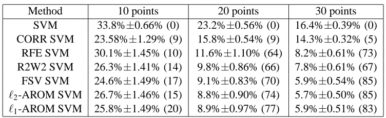
In this problem the first six features have redundancy and the rest of the features are irrelevant. We used linear decision rules and for feature selection we selected the 2 best features. We trained on 10, 20 and 30 randomly drawn training points, testing on a further 500 points, and averaging test error over 100 trials. The results are given in Table 1. For each technique the test error and standard error is given. For 20 or more training points, AROM SVMs outperform RFE, R2W2 and CORR SVMs whereas conventional SVMs overfit. Note that for very small training set sizes (e.g. size 10) the number of times that two relevant and non-redundant features are chosen (given in brackets in the figure) is not completely correlated with the test error. This can happen when it is “easier” for an algorithm to choose two relevant and redundant features (as in CORR) than to try to find the non-redundant ones.

Method 10 points 20 points 30 points

SVM 33.8%±0.66% (0) 23.2%±0.56% (0) 16.4%±0.39% (0) CORR SVM 23.58%±1.29% (9) 15.8%±0.54% (9) 14.3%±0.32% (5) RFE SVM 30.1%±1.45% (10) 11.6%±1.10% (64) 8.2%±0.61% (73) R2W2 SVM 26.3%±1.41% (14) 9.8%±0.86% (66) 7.8%±0.61% (67) FSV SVM 24.6%±1.49% (17) 9.1%±0.83% (70) 5.9%±0.54% (85) `2-AROM SVM 26.7%±1.46% (15) 8.8%±0.90% (74) 5.7%±0.50% (85) `1-AROM SVM 25.8%±1.49% (20) 8.9%±0.97% (77) 5.9%±0.51% (83)

Table 1: Feature selection on a linear problem. AROM SVMs (using both the `1 and `2 multi-plicative updates) outperform RFE, R2W2 and CORR SVMs, other techniques of feature selection in the case where conventional SVMs overfit. For each technique the percentage test error and standard error is given. In brackets is the number of times that two relevant and non-redundant features are chosen. See the text for more details.

We measured the significance of these results using the Wilcoxon signed rank test with a signif-icance levelα=0.05. The results show that the`1-AROM SVM,`2-AROM SVM and FSV SVM are significantly better than all the other methods for training set sizes 30 with a p-value less than 0.005 but are not significantly different from each other. For training set size 20, R2W2 SVM is also not significantly different to these best performing algorithms (but significantly outperforms the others).

We also compared these methods with some “naive” wrapper feature selection methods using the `1- or `2- norm: choose the two largest values of |wi| as the features of choice. This is in effect using only the first iteration of the AROM (or RFE) algorithm, and as such represents a sanity check that the iterative procedure does improve the quality of the chosen features. In fact these naive

(16)

methods perform similarly to the CORR SVM: the`2-norm yields for 10, 20 and 30 training points: 26.8%±1.39 (3), 16.302%±0.77042 (16) and 13.4%±0.42 (17). The`1-norm yields: 25.9%±1.45 (17), 11.008%±1.0921 (67) and 12.1%±1.35 (66).

Two-class Microarray datasets We then performed experiments on real-life problems. For DNA microarray data analysis one needs to determine the relevant genes in discrimination as well as discriminate accurately. We look at a problem of distinguishing between cancerous and normal tissue in a colon cancer problem examined by Alon et al. (1999) (see also Guyon et al. 2001 for a treatment of this problem) and in a large B-Cell lymphoma problem described by Alizadeh (2000). In the colon cancer problem, 62 tissue samples probed by oligonucleotide arrays contain 22 normal and 40 colon cancer tissues that must be discriminated based upon the expression of 2000 genes. Splitting the data into a training set of 50 and a test set of 12 in 500 separate trials we obtained a test error of 13.89% for standard linear SVMs. We then measured the test error of SVMs trained with features chosen by five input selection methods: CORR, RFE, R2W2, FSV and our approach, `2–AROM. We chose subsets of 2000, 1000, 500, 250, 100, 50 and 20 genes. The results are shown in Table 2.

Feats. CORR SVM RFE SVM R2W2 SVM FSV SVM `2–AROM

2000 13.89%±1.6% 13.89%±1.6% 13.89%±1.6% 13.89%±1.6% 13.89%±1.6% 1000 14.44%±1.6% 13.89%±1.6% 14.17%±1.5% 16.11%±1.5% 14.17%±1.6% 500 16.39%±1.9% 13.06%±1.4% 12.78%±1.6% 15.56%±1.8% 14.17%±1.3% 250 15.28%±1.7% 12.78%±1.4% 12.78%±1.6% 14.17%±1.7% 13.61%±1.6% 100 16.94%±1.7% 13.06%±1.7% 12.5%±1.7% 14.17%±2.2% 11.94%±1.9% 50 21.67%±1.6% 12.5%±1.5% 11.11%±1.7% 16.39%±2.1% 11.11%±1.7% 20 32.5%±2.6% 14.44%±1.7% 14.44%±2.1% 16.67%±2.2% 14.17%±2%

Table 2: Input selection on micro-array data colon cancer vs normal. The average percentage test error over 30 splits is given for various numbers of genes selected using five approaches.

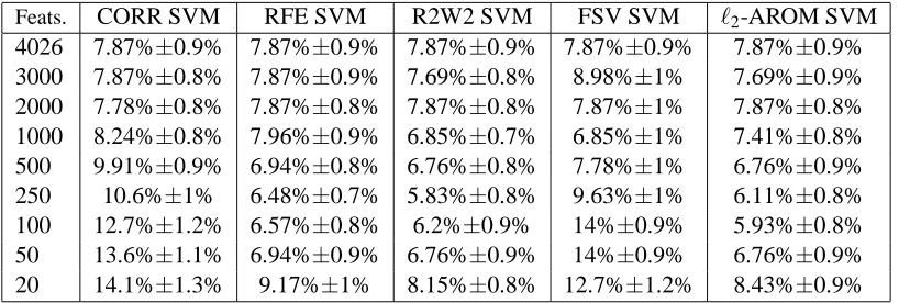
Feats. CORR SVM RFE SVM R2W2 SVM FSV SVM `2-AROM SVM

4026 7.87%±0.9% 7.87%±0.9% 7.87%±0.9% 7.87%±0.9% 7.87%±0.9% 3000 7.87%±0.8% 7.87%±0.9% 7.69%±0.8% 8.98%±1% 7.69%±0.9% 2000 7.78%±0.8% 7.87%±0.8% 7.87%±0.8% 7.87%±1% 7.87%±0.8% 1000 8.24%±0.8% 7.96%±0.9% 6.85%±0.7% 6.85%±1% 7.41%±0.8% 500 9.91%±0.9% 6.94%±0.8% 6.76%±0.8% 7.78%±1% 6.76%±0.9% 250 10.6%±1% 6.48%±0.7% 5.83%±0.8% 9.63%±1% 6.11%±0.8% 100 12.7%±1.2% 6.57%±0.8% 6.2%±0.9% 14%±0.9% 5.93%±0.8% 50 13.6%±1.1% 6.94%±0.9% 6.76%±0.9% 14%±0.9% 6.76%±0.9% 20 14.1%±1.3% 9.17%±1% 8.15%±0.8% 12.7%±1.2% 8.43%±0.9%

(17)

In this experiment we can no longer use the Wilcoxon signed rank test to assess significance because the trials are dependent. We therefore used the corrected resampled t-test statistic of Nadeau and Bengio (2001) which is a test developed to attempt to take this dependence into account. In fact, taking a confidence level of α=0.05 the test showed that none of the differences between algorithms were significant – apart from between CORR SVM and the other algorithms for feature size 20. Note that the Wilcoxon test, on the other hand, returns that many of the differences are significant. This serves to highlight the difficulty of assessing significance with such small dataset sizes.

In the lymphoma problem the gene expression of 96 samples is measured with microarrays to give 4026 features, 61 of the samples are in classes ”DLCL”, ”FL” or ”CLL” (malignant) and 35 are labelled “otherwise” (usually normal). We followed the same approach as in the colon cancer problem, splitting the data this time into training sets of size 60 and test sets of size 36 over 30 separate trials. The results are given in Table 3. Similarly to the colon cancer experiment, the corrected resampled t-test statistic returned that none of the differences between algorithms were significant.

To give an idea of the relative training times of the methods we computed the CPU time of one training run on the lymphoma dataset. We obtained the following times: FSV: 139.34 seconds, `2-AROM SVM: 2.39 seconds, RFE (choosing 20 features): 1.22 seconds, SVM: 0.34 secs, CORR: 0.27 secs. Clearly computational efficiency is not accurately measured by computer time if the algorithms are not optimized. Yet we think this provides an idea of the computational efficiency, e.g. the difference between FSV and`2-AROM SVM (which both try to minimize the zero-norm) is due to the inability of FSV to take advantage of dual optimization and so scales with respect to the number of features, rather the number of training patterns.

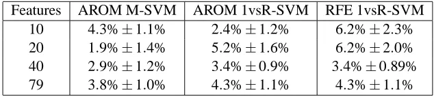
Features AROM M-SVM AROM 1vsR-SVM RFE 1vsR-SVM 10 4.3%±1.1% 2.4%±1.2% 6.2%±2.3% 20 1.9%±1.4% 5.2%±1.6% 6.2%±2.0% 40 2.9%±1.2% 3.4%±0.9% 3.4%±0.89% 79 3.8%±1.0% 4.3%±1.1% 4.3%±1.1%

Table 4: Result of the feature selection preprocessing on the Brown-Yeast dataset: 5 classes, 208 training points of dimension 79. The percentages represent the fraction of errors using 8 fold cross validation, as well as their standard errors. The number of features used by the methods is also given. M-SVM means multiclass SVM and 1vsR stands for one-against-the-rest. The AROM is performed with the`2approximation.

(18)

`2-AROM procedure. Finally, we also ran a one-against-the-rest SVM combined with RFE. Table 4 presents the result. Note that the performance of the learning system combined with AROM for feature selection improves generalization performance. Being able to reduce the number of features while having lower or the same generalization error allows the user to focus on a limited amount of information and to check whether this information is relevant or not. It is worth noticing also that the performance of the one-against-the-rest approach is improved when selecting only 40 features with the RFE method. The number of features is however larger than with the AROM procedure. Thus both in terms of identifying a small number of useful features and improving generalization ability, AROM seems to be preferable to RFE. However we expect the number of trials performed here to be too small to suggest the significance of these results.

4.6 Discussion

We have shown how the zero-norm minimization can be used for feature selection, and have com-pared it to some existing feature selection methods. It performs about as well as the best alternative method compared on some specific microarray problems.

When comparing feature selection algorithms, the generalizaton performance is not the only reason for choosing a particular method. Some key differences between the methods include:

• Computational efficiency. Of the algorithms tested correlation scores are the fastest to com-pute, then methods that use dual optimization (which is possible with the two-norm) such as SVM, RFE and `2-AROM, whereas the slowest are the methods which minimize the one-norm such as FSV and`1-AROM SVM.

• Applicability to Nonlinear problems. Of the methods tested, only R2W2 and RFE are appli-cable for choosing features in input space relevant for nonlinear problems.

• Capacity. By searching the space of subsets of features wrapper approaches (e.g. RFE) and the zero-norm minimization can more effectively minimize the training error than filter methods such as CORR. Hence in some sense they have a higher capacity. The applicability of these algorithms thus depends upon the complexity of the problem at hand: filter methods can underfit complex data (e.g. CORR can fail if the data are multivariate or nonlinear) whereas the other methods can overfit the data. Clearly, choosing features via a criterion such as cross validation error or a generalization bound can bias the estimate of the criterion through its minimization in just then same way as training error is a biased measure of generalization ability after minimizing it. As a final remark this means that even though methods such as RFE and even the AROM methods end up being forms of backward selection which do not search through the whole space of possible subsets this is not necessarily a bad thing in that their capacity is thus not as high as a more complete search of the space (which as well as overfitting, would be computational less tractable anyway).

Several other issues are noteworthy:

(19)

parameter can be already expensive to compute) could be difficult without somehow solving both problems at once. Furthermore, as many approaches, e.g. wrapper approaches have al-ready used an estimate of generalization error to select features it makes using the same or related measures more biased and thus less effective for this task.

• Model selection: other parameters. For SVMs it would also be nice to be able to select the other parameters (kernel parameters, soft margin parameter C) at the same times as the number of features. Of the techniques described only R2W2 provides an obvious mechanism for doing this.

• The goal of feature selection. In this work we have concentrated on the goal of choosing features such that generalization error is minimized. However, this is not always of interest: for example the goal may be to know which features would be (the most) relevant features if the optimal decision function were known. In microarray data, which we have focussed on, the true goal is often more application specific than what we have addressed. One may be interested in finding genes which are potential drug targets. Filter methods such as correlation scores are thus often preferred because they return a ranked list of (possibly redundant) genes (rather than subsets) which are highly correlated with the labels. The redundancy in this case can be beneficial due to application specific constraints (e.g. usefulness of this gene as a drug target). However, in the future choosing subsets of genes may become more important, especially as the amount of available data increases, making such (more difficult) problems feasible

5. Nonlinear Feature Selection via Kernels

In the nonlinear feature selection problem one would like to select a subset of features in the space induced by a kernel, usually with the aim of improving the discriminative ability of a classifier (see Section 3.4 for the details of how to apply the zero-norm to this problem).

An example of the use of such a method would be an application where the data require one to use a nonlinear decision rule (e.g. a polynomial) but the best decision rule is sparse in the param-eters of the nonlinear rule (e.g. a sparse polynomial). For example, one possible application could thus be image recognition, where not all polynomial terms are expected to have nonzero weight (e.g. terms involving pixels far away from each other). However, in this case it might be better to explicitly implement this prior knowledge into the construction of the kernel. In this section we only demonstrate the effectiveness of this method on toy examples.

5.1 Experimental Results

We compared the zero-norm minimization to the solution of SVMs on some general nonlinear toy problems. Note that we do not compare to conventional feature selection methods because if w is too large in dimension these methods can no longer be easily used. We chose input spaces of dimension n=10 and a mapping into feature space of polynomial of degree 2:φ(x) =φ1:2(x). The

(20)

20 40 60 80 100 0 0.05 0.1 0.15 0.2 0.25 0.3 0.35 Training pts Error

f(x) = x1 x2+x3

f(x) = x1

(a) (b)

95% sparse poly degree 2

(c) (d)

20 40 60 80 100

0 0.1 0.2 0.3 0.4 0.5 Training pts Error

(e) (f)

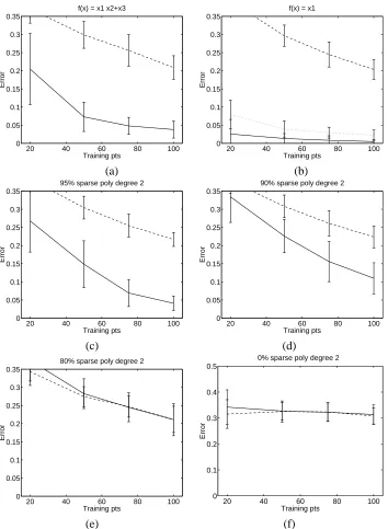
Figure 1: A comparison of SVMs (dashed lines) and the`2-AROM SVM (solid lines) for learning sparse and non-sparse target functions with polynomials of degree 2 over 10 inputs. The `2-AROM SVM outperforms the SVM solution if the target is sparse, and gives compara-ble performance otherwise. When the target is a sparse linear target the`2-AROM SVM even outperforms a linear SVM (dotted lines). See the text for details.

(21)

possible if w is large) we found the performance was identical. We do not believe this will always be the case: if the required solution does not exist in the span of the training vectors then Equation (25) in Appendix C of Weston et al. (2001a) could be a poor approximation. Results are shown in Figure 1.

In problems (a)-(d) the `2-AROM SVM method clearly outperforms SVMs. This is due to the norm that SVMs use, the`2-norm which places a preference on using as many coefficients as possible in its decision rule. This is costly when the number of features one should use is small. In problem (b) where the decision rule to be learned is linear (just one feature) the difference is the largest. On this problem the dotted lines in the plot represent the performance of a linear SVM (as the target is linear). The linear SVM outperforms the polynomial SVM, as one would expect, but surprisingly the AROM feature selection method in the space of polynomial coefficients of degree two still outperforms the linear SVM. This is again because the linear SVM, using the`2-norm does not perform feature selection.

Finally, problems (e) and (f) show an 80% and 0% sparse target respectively. Note that although our method outperforms SVMs in the case of sparse targets it is not much worse (in this example at least) when the target is not sparse, as in problem (f). Note that is not the case in the micro-array analysis of the previous section, the feature selection degrades performance when the number of features becomes too small even though the data are still linearly separable.

6. Final Discussion and Conclusions

In conclusion we have introduced a simple optimization technique for minimizing the zero-norm and have studied several applications of the zero-norm in machine learning. The main advantage of our algorithm over existing ones is its computational advantage when the number of variables exceeds the number of examples. In particular, we are able to use existing speedup methods and heuristics that have been designed for SVM and to use them to minimize the zero-norm. It allows one to handle large data sets with relatively small computer resources as has been shown in the original papers (e.g. Osuna et al., 1997a,b). It is also simple to adapt our method to different domains, as shown in the applications. We have shown how it can be useful in terms of feature selection (when one is interested in discovering features) and pattern recognition (for obtaining good generalization performance). In related work (Weston et al., 2001a), we also show how to use it for obtaining sparse representations and for compression (vector quantization) on both toy and real-life problems. The usefulness of the minimization of the zero-norm in general depends on the type of problem. In vector quantization and feature selection problems the method’s usefulness is clear, since sparsity is an explicit goal in these applications. In pattern recognition it depends on the (unknown) target. For example: are your data such that a rule using just a small number of features yields good performance? Are there many irrelevant features (noise)? In these cases the zero-norm can be very useful. Constructing toy examples of this type shows one can obtain large performance gains selecting the appropriate norm, for example in Figure 1. However, the nature of the `0-norm as a regularizer is not completely clear, in our experiments we trained a subsequent `2-norm classifier on the chosen features, giving improved performance. Part of the problem is that the`0-norm does not have a unique solution. Trading off the number of variables with badness of fit is perhaps not really enough to produce good classifiers and a third (regularization) term is in fact necessary.

(22)

multi-label categorisation (where each example may belong to one or many categories), in regres-sion, and in time series analysis. We plan to further research these kinds of system which are of particular importance in a growing number of real-world applications, especially in the domain of bioinformatics.

References

M. Aizerman, E. Braverman, and L. Rozonoer. Theoretical foundations of the potential function method in pattern recognition learning. Automation and Remote Control, 25:821 – 837, 1964.

A.A. Alizadeh. Distinct types of diffues large b-cell lymphoma identified by gene expression profiling.

Nature, 403:503–511, 2000.

U. Alon, N. Barkai, D. Notterman, K. Gish, S. Ybarra, D. Mack, and A. Levine. Broad patterns of gene expression revealed by clustering analysis of tumor and normal colon cancer tissues probed by oligonu-cleotide arrays. Cell Biology, 96:6745–6750, 1999.

E. Amaldi and V. Kann. On the approximability of minimizing non zero variables or unsatisfied relations in linear systems. Theoretical Computer Science, 209:237–260, 1998.

K. P. Bennett and O. L. Mangasarian. Robust linear programming discrimination of two linearly inseparable sets. Optimization Methods and Software, 1:23–34, 1992.

A. Blum and P. Langley. Selection of relevant features and examples in machine learning. Artificial

Intelli-gence, 97:245–271,, 1997.

B. Boser, I. Guyon, and V. Vapnik. A training algorithm for optimal margin classifiers. In Fifth Annual

Workshop on Computational Learning Theory, pages 144–152, Pittsburgh, 1992. ACM.

P. S. Bradley and O. L. Mangasarian. Feature selection via concave minimization and support vector ma-chines. In Proc. 13th ICML, pages 82–90, San Francisco, CA, 1998.

P. S. Bradley and O. L. Mangasarian. Massive data discrimination via linear support vector machines.

Opti-mization Methods and Software, 13(1):1–10, 2000. URLciteseer.nj.nec.com/bradley98massive. html.

P. S. Bradley, O. L. Mangasarian, and W. N. Street. Feature selection via mathematical programming. Tech-nical Report 95-21, Computer Sciences Department, University of Wisconsin, Madison, Wisconsin, 1995. To appear in INFORMS Journal on Computing 10, 1998.

C. Cortes and V. Vapnik. Support vector networks. Machine Learning, 20:273 – 297, 1995.

R. Courant and D. Hilbert. Methods of Mathematical Physics, volume 1. Interscience Publishers, Inc, New York, 1953.

M. Franke and P. Wolfe. An algorithm for quadratic programming. Naval Research Logistics Quarterly 3, pages 95–110, 1956.

Y. Freund and R. Schapire. Large margin classification using the perceptron algorithm. In COLT, 1998.

G. Fung, O. L. Mangasarian, and A. J. Smola. Minimal kernel classifiers. Technical Report DMI-00-08, Data Mining Institute, University of Wisconsin, Madison, 2000. Submitted to IEEE Transactions on Pattern

(23)

I. Guyon, J. Weston, S. Barnhill, and V. Vapnik. Gene selection for cancer classification using support vector machines. Machine Learning, 2001.

O.L. Mangasarian. Linear and nonlinear separation of patterns by linear programming. Operations Research, 13:444–452, 1965.

C. Nadeau and Y. Bengio. Inference for the generalization error. Machine Learning, 2001.

R. M. Neal. Assessing relevance determination methods using delve. Neural Networks and Machine

Learn-ing, pages 97–129, 1998.

E. Osuna, R. Freund, and F. Girosi. An improved training algorithm for support vector machines. In Neural

Networks for Signal Processing VII - Proceedings of the 1997 IEEE Workshop, pages 276–285, New-York,

1997a. IEEE.

E. Osuna, R. Freund, and F. Girosi. Training support vector machines: An application to face detection. In

IEEE Computer Society Conference on Computer Vision and Pattern Recognition, Los Alamos, 1997b.

Computer Society.

F. Pérez-Cruz, A. Navia-Vázquez, A. R. Figueiras-Vidal, and A. Artés-Rodr´ıguez. Empirical risk minimiza-tion for support vector machines. IEEE Transacminimiza-tion on Neural Networks, 2002. Submitted for publicaminimiza-tion.

F. Rosenblatt. The perceptron: A probabilistic model for information storage and organization in the brain.

Psychological Review, 65(6):386–408, 1958.

B. Sch¨olkopf and A. J. Smola. Learning with Kernels. MIT Press, Cambridge, MA, 2002.

E. Takimoto and M. Warmuth. Series parallel kernels and an application to multiplicative updates. NIPS

2000 Workshop on New perspectives in Kernel based methods, 2000.

M. E Tipping. Sparse Bayesian learning and the relevance vector machine. Journal of Machine Learning

Research, 1:211–244, 2001.

V. Vapnik. Estimation of Dependences Based on Empirical Data [in Russian]. Nauka, Moscow, 1979. (English translation: Springer Verlag, New York, 1982).

V. Vapnik. The Nature of Statistical Learning Theory. Springer Verlag, New York, 1995.

V. Vapnik. Statistical Learning Theory. John Wiley and Sons, New York, 1998.

J. Weston, A. Elisseeff, and B. Sch ¨olkopf. Use of the`0-norm with linear models and kernel methods.

Technical report, 2001a. http://www.kyb.tuebingen.mpg.de/bs/people/weston/l0.

J. Weston, S. Mukherjee, O. Chapelle, M. Pontil, T. Poggio, and V. Vapnik. Feature selection for svms. In

Neural Information Processing Systems, Cambridge, MA, 2001b. MIT Press.