Sparse Spectrum Gaussian Process Regression

(1)

Sparse Spectrum Gaussian Process Regression

Miguel Lázaro-Gredilla [email protected]

Departamento de Teoría de la Señal y Comunicaciones Universidad Carlos III de Madrid

28911 Leganés, Madrid, Spain

Joaquin Quiñonero-Candela [email protected]

Microsoft Research Ltd. 7 J J Thomson Avenue Cambridge CB3 0FB, UK

Carl Edward Rasmussen∗ [email protected]

Deparment of Engineering

University of Cambridge, Trumpington st. Cambridge CB2 1PZ, UK

Aníbal R. Figueiras-Vidal [email protected]

Departamento de Teoría de la Señal y Comunicaciones Universidad Carlos III de Madrid

28911 Leganés, Madrid, Spain

Editor: Tommi Jaakkola

Abstract

We present a new sparse Gaussian Process (GP) model for regression. The key novel idea is to sparsify the spectral representation of the GP. This leads to a simple, practical algorithm for regres-sion tasks. We compare the achievable trade-offs between predictive accuracy and computational requirements, and show that these are typically superior to existing state-of-the-art sparse approx-imations. We discuss both the weight space and function space representations, and note that the new construction implies priors over functions which are always stationary, and can approximate any covariance function in this class.

Keywords: Gaussian process, probabilistic regression, sparse approximation, power spectrum, computational efficiency

1. Introduction

One of the main practical limitations of Gaussian processes (GPs) for machine learning (Rasmussen and Williams, 2006) is that in a direct implementation the computational and memory requirements

scale as

O

(n2)and

O

(n3), respectively. In practice this limits the applicability of exact GP

imple-mentations to data sets where the number of training samples n does not exceed a few thousand. A number of computationally efficient approximations to GPs have been proposed, which

re-duce storage requirements to

O

(nm)and the number of computations to

O

(nm2), where m is much

smaller than n. One family of approximations, reviewed in Quiñonero-Candela and Rasmussen (2005), is based on assumptions of conditional independence given a reduced set of m inducing

(2)

inputs. Examples of such models are those proposed in Seeger et al. (2003), Smola and Bartlett

(2001), Tresp (2000), Williams and Seeger (2001) and Csató and Opper (2002), as well as the Fully Independent Training Conditional (FITC) model, introduced as Sparse Pseudo-input GP (SPGP) by Snelson and Ghahramani (2006). Walder et al. (2008) introduced the Sparse Multiscale GP (SMGP), a modification of FITC that allows each basis function to have its own set of

length-scales.1 This additional flexibility typically yields some performance improvement over FITC, but

it also requires learning twice as many parameters. SMGP can alternatively be derived within the unifying framework of Quiñonero-Candela and Rasmussen (2005) if we allow the inducing inputs to lie in a transformed domain, as shown in Lázaro-Gredilla and Figueiras-Vidal (2010).

Another family of approximations is based on approximate matrix-vector-multiplications (MVMs), where m is for example a reduced number of conjugate gradient steps to solve a sys-tem of linear equations. Some of these methods have been briefly reviewed in Quiñonero-Candela et al. (2007). Local mixtures of GP have been used by Urtasun and Darrell (2008) for efficient modelling of human poses.

In this paper we introduce a stationary trigonometric Bayesian model for regression that retains the computational efficiency of the aforementioned approaches, while improving performance. The model consists of a linear combination of trigonometric functions where both weights and phases are integrated out. All hyperparameters of the model (frequencies and amplitudes) are learned jointly by maximizing the marginal likelihood. This model is a stationary sparse GP that can approximate any desired stationary full GP. Sparse trigonometric expansions have been proposed in several contexts, for example, Lázaro-Gredilla et al. (2007) and Rahimi and Recht (2008), as discussed further in Section 4.3.

FITC, SMGP, and the model introduced in this paper focus on predictive accuracy at low com-putational cost, rather than on faithfully converging towards the full GP as the number of basis func-tions grows. Performance-wise, FITC and the more recent SMGP can be regarded as the current state-of-the-art sparse GP approximations, so we will use them as benchmarks in the performance comparisons.

In Section 2 we give a brief review of GP regression. In Section 3 we introduce the trigono-metric Bayesian model, and in Section 4 we present the Sparse Spectrum Gaussian Process (SSGP) algorithm. Section 5 contains a comparative performance evaluation on several data sets.

2. Gaussian Process Regression

Regression is often formulated as the task of predicting the scalar output y∗ associated to the

D-dimensional input x∗, given a training data set

D

≡ {xj,yj|j=1, . . .n}of n input-output pairs. A

common approach is to assume that the outputs have been generated by an unknown latent function

f(x)and independently corrupted by additive Gaussian noise of constant varianceσ2_n:

yj = f(xj) +εj, εj ∼

N

(0,σ2n).

The regression task boils down to making inference about f(x). Gaussian process (GP) regression

is a probabilistic, non-parametric Bayesian approach. A Gaussian process prior distribution on f(x)

allows us to encode assumptions about the smoothness (or other properties) of the latent function

(3)

(Rasmussen and Williams, 2006). For any set of inputs{xi}n

i=1the corresponding vector of function

evaluations f= [f(x1), . . . ,f(xn)]⊤has a joint Gaussian distribution:

p(f|{xi}ni=1) =

N

(f|0,Kff).

This paper follows the common practice of setting the mean of the process to zero.2 The properties

of the GP prior over functions are governed by the covariance function

Kff

i j = k(xi,xj) = E[f(xi)f(xj)], (1)

which determines how the similarity between a pair of function values varies as a function of the corresponding pair of inputs. A covariance function is stationary if it only depends on the difference between its inputs

k(xi,xj) = k(xi−xj) = k(τ).

The elegance of the GP framework is that the properties of the function are conveniently expressed directly in terms of the covariance function, rather than implicitly via basis functions.

To obtain the predictive distribution p(y∗|x∗,

D

) it is useful to express the model in matrix

notation by stacking the targets yj in vector y= [y1, . . . ,yn]⊤ and writing the joint distribution of

training and test targets:

y y∗

∼

N

0,

Kff+σ2nIn kf∗

k⊤_f_∗ k∗∗+σ2n

,

where kf∗ is the vector of covariances between f(x∗) and the training latent function values, and

k∗∗is the prior variance of f(x∗). Inis the n×n identity. The predictive distribution is obtained by

conditioning on the observed training outputs:

p(y∗|x∗,

D

) =

N

(µ∗,σ2∗), where

µ∗=k∗f(Kff+σ2nIn)−1y

σ2

∗=σ2n+k∗∗−k∗f(Kff+σ2nIn)−1kf∗. (2) The covariance function is parameterized by hyperparameters. Consider for example the sta-tionary anisotropic squared exponential covariance function

kARD(τ) = σ20exp(−12τ

⊤_Λ−1_τ₎_, _where _Λ ₌ _diag([_ℓ2

1, ℓ22, . . . ℓ2D]). (3)

The hyperparameters are the prior varianceσ2₀and the lengthscales{ℓd}that determine how rapidly

the covariance decays with the distance between inputs. This covariance function is also known as the ARD (Automatic Relevance Determination) squared exponential, because it can effectively prune input dimensions by growing the corresponding lengthscales.

It is convenient to denote all hyperparameters including the noise variance byθ. These can be

learned by maximizing the evidence, or log marginal likelihood:

log p(y|θ) = −n

2log(2π)−

1

2|Kff+σ

2 nIn| −

1

2y

⊤ _K

ff+σ2nIn

−1

y. (4)

Provided there exist analytic forms for the gradients of the covariance function with respect to the hyperparameters, the evidence can be maximized by using a gradient-based search. Unfortunately,

computing the evidence and the gradients requires the inversion of the covariance matrix Kff+σ2nIn

at a cost of

O

(n3)operations, which is prohibitive for large data sets.

(4)

3. Trigonometric Bayesian Regression

In this section we present a Bayesian linear regression model with trigonometric basis functions, and related it to a full GP in the next section. Consider the model

f(x) =

m

∑

r=1

arcos(2πs⊤_rx) +brsin(2πs⊤_rx), (5)

where each of the m pairs of basis functions is parametrized by a D-dimensional vector srof spectral

frequencies. Note that each pair of basis functions share frequencies, but each have independent

amplitude parameters, ar and br. We treat the frequencies as deterministic parameters and the

amplitudes in a Bayesian way. The priors are independent Gaussian

ar ∼

N

0,

σ2 0 m

, br ∼

N

0,

σ2 0 m

,

where the variances are scaled down linearly by the number of basis functions. Under the prior, the distribution over functions from Equation (5) is Gaussian with mean function zero and covariance function (from Equation (1))

k(xi,xj) =

σ2 0 mφ(xi)

⊤_φ₍_x

j) =

σ2 0 m m

∑

r=1

cos 2πs⊤_r(xi−xj)

, (6)

where we define the column vector of length 2m containing the evaluation of the m pairs of trigono-metric functions at x

φ(x) =

cos(2πs⊤₁x) sin(2πs⊤₁x) . . . cos(2πs⊤_mx) sin(2πs⊤_mx)⊤

.

Sparse linear models generally induce priors over functions whose variance depends on the input. In contrast, the covariance function in Equation (6) is stationary, that is, the prior variance is

inde-pendent of the input and equal toσ2₀. This is due to the particular nature of the trigonometric basis

functions and implies that the predictive variances cannot be “healed”, as proposed in Rasmussen and Quiñonero-Candela (2005) for the case of the Relevance Vector Machine.

The predictions and marginal likelihood can be evaluated using Equations (2) and (4), although

direct evaluation is computationally inefficient when 2m<n. For the predictive distribution we use

the more efficient

E[y∗] = φ(x∗)⊤A−1Φfy, V[y∗] = σ2n+σ2nφ(x∗)⊤A−1φ(x∗), (7)

where we have defined the 2m by n design matrixΦf= [φ(x1), . . . ,φ(xn)]and A=ΦfΦ⊤f +

mσ2

n

σ2 0

I2m.

Similarly, for the log marginal likelihood

log p(y|θ) = −

y⊤y−y⊤Φ⊤_f A−1Φfy

/(2σ2 n)−

1

2log|A|+m log

mσ2 n

σ2 0

−n

2log 2πσ

2

n. (8)

A stable and efficient implementation uses Cholesky decompositions, Appendix A. Both the

predic-tive distribution and the marginal likelihood can be computed in

O

(nm2). The predictive mean and

variance at an additional test point can be computed in

O

(m) and

O

(m2_{) respectively. The storage}

costs are also reduced, since we no longer store the full covariance matrix (of size n×n), but only

(5)

3.1 Periodicity

One might be tempted to assume that this model would only be useful for modeling periodic func-tions, since strictly speaking a linear combination of periodic signals is itself periodic. However, if the individual frequencies are not all multiples of a common base frequency, then the period of the resulting signal will be very long, typically exceeding the range of the inputs by orders of magnitude. Thus, the model based on trigonometric basis functions has practical use for modeling non-periodic functions. The same principle is used (interchanging input and frequency domains) in uneven sampling to space apart frequency replicas an avoid aliasing, see for instance Bretthorst (2000). As our experimental results suggest, the model provides satisfactory predictive variances.

3.2 Representation

An alternative and equivalent representation of the model in Equation (5), which only uses half the number of trigonometric basis functions is possible, by writing the linear combination of a sine and a cosine as a cosine with an amplitude and a phase. Although these two representations are equivalent, inference based on them differs. Whereas we have been able to integrate out the amplitudes to arrive at the GP in Equation (6), this would not be possible analytically using the more parsimonious representation.

Optimization instead of marginalization of the phases has two important consequences. Firstly, we lose the property of stationarity of the prior over functions. Secondly we may expect that the model becomes more prone to overfitting. When considering the contribution from a basis func-tion (pair) with a specific frequency, the optimizafunc-tion based scheme could fit arbitrarily the phase, whereas the integration based inference is constrained to use a flat prior over phases. In Section 5.3 we empirically verify that the computation vs accuracy tradeoff typically favors the less compact representation.

4. The Sparse Spectrum Gaussian Process

In the previous section we presented an explicit basis function regression model, but we did not dis-cuss how to select the frequencies defining the basis functions. In this section, we present a sparse GP approximation view of this model, which shows how it can be understood as a computation-ally efficient approximation to any GP with stationary covariance function. In the next section we present experimental results showing that dramatic improvements over other state-of-the-art sparse GP regression algorithms are possible.

We will now take a generic GP with stationary covariance function and sparsify its power spec-tral density to obtain a sparse GP that approximates the full GP. The power specspec-tral density (or power

spectrum) S(s)of a stationary random process expresses how the power is distributed over the

fre-quency domain. For a stationary GP, the power is equal to the prior variance k(x,x) =k(0) =σ2

0.

The frequency vector s has the same length D as the input vector x. The d-th element of s can be in-terpreted as the frequency associated to the d-th input dimension. The Wiener-Khintchine theorem (see for example Carlson, 1986, p. 162) states that the power spectrum and the autocorrelation of

the random process constitute a Fourier pair. In our case, given that f(·)is drawn from a stationary

Gaussian process, the autocorrelation function is equal to the stationary covariance function, and we have:

k(τ) = Z

RDe

2πis⊤τ_S₍_s₎_ds, _S₍_s_{) =} Z

RDe

(6)

We thus see that there are two equivalent representations for a stationary Gaussian process: the traditional one in terms of the covariance function in the (input) space domain, and a perhaps less usual one as the power spectrum in the frequency domain.

Bochner’s theorem (Stein, 1999, p. 24) states that any stationary covariance function k(τ)can

be represented as the Fourier transform of a positive finite measure. This means that the power spectrum in (9) is a positive finite measure, and in particular that it is proportional to a probability

measure, S(s) ∝pS(s). The proportionality constant can be directly obtained by evaluating the

covariance function in (9) atτ=0. We obtain the relation:

S(s) = k(0)pS(s) = σ2₀pS(s). (10)

We can use the fact that S(s)is proportional to a multivariate probability density in s to rewrite the

covariance function in (9) as an expectation:

k(xi,xj) = k(τ) = Z

RDe

2πis⊤(xi−xj)_S₍_s₎_ds ₌ _σ2 0 Z

RDe

2πis⊤xi_e2πis⊤xj∗_pS₍_s₎_ds

= σ2 0EpS

h

e2πis⊤xie2πis⊤xj∗i_, ₍₁₁₎

whereE_p

S denotes expectation wrt. pS(s) and superscript asterisk

3 _{denotes complex conjugation.}

This last expression is an exact expansion of the covariance function as the expectation of a product of complex exponentials with respect to a particular distribution over their frequencies. This integral can be approximated by simple Monte Carlo by taking an average of a few samples corresponding to a finite set of frequencies, which we call spectral points.

Since the power spectrum is symmetric around zero, a valid Monte Carlo procedure is to sample

frequencies always as a pair{sr,−sr}. This has the advantage of preserving the property of the exact

expansion, Equation (11) that the imaginary terms cancel:

k(xi,xj) ≃

σ2 0 2m m

∑

r=1 h

e2πis⊤rxi

e2πis⊤rxj∗₊_e2πis⊤rxi

∗

e2πis⊤rxj

i = σ 2 0 mRe h m

∑

r=1 e2πis⊤rxi

e2πis⊤rxj

∗i = σ 2 0 m m

∑

r=1

cos 2πs⊤_r(xi−xj)

,

where sr is drawn from pS(s) and Re[·]denotes the real part of a complex number. Notice, that

we have recovered exactly the expression for the covariance function induced by the trigonometric basis functions model, Equation (6). Further, we have given an interpretation of the frequencies as spectral Monte Carlo samples, approximating any stationary covariance function. This is a more general result than that of (MacKay, 2003, Ch. 45), which only applies to Gaussian covariances.

The approximation is equivalent to replacing the original spectrum S(s)by a set of Dirac deltas of

amplitudeσ2₀distributed according to pS(s). Thus, we “sparsify” the spectrum of the GP.

This convergence result can also be stated as follows: A stationary GP can be seen as a neural network with infinitely many hidden units and trigonometric activations if independent priors

fol-lowing Gaussian and pS(s) distributions are placed on the output and input weights, respectively.

(7)

−8 −6 −4 −2 0 2 4 6 8 −0.4

−0.2 0 0.2 0.4 0.6 0.8 1 1.2

τ

Covariance function

SE covariance function 10 spectral points approx.

−8 −6 −4 −2 0 2 4 6 8

−0.4 −0.2 0 0.2 0.4 0.6 0.8 1 1.2

τ

Covariance function

SE covariance function 50 spectral points approx.

(a) (b)

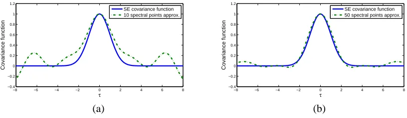
Figure 1: Squared exponential covariance function and its approximation with (a) 10 and (b) 50 random spectral points respectively.

4.1 Example: The Squared Exponential Covariance Function

The probability density associated to the squared exponential covariance function of Equation (3) can be obtained from the Fourier transform

pARD_S (s) = 1

kARD(0) Z

RDe

−2πis⊤τ_kARD₍_τ₎_d_τ ₌ p

|2πΛ|exp(−2π2s⊤Λs), (12) which also has the form of a multivariate Gaussian distribution. For illustration purposes, we com-pare the exact squared exponential covariance function with its spectral approximation in Figure 1, where the spectral points are sampled from Equation (12). As expected, the quality of the approxi-mation improves with the number of samples.

4.2 The SSGP Algorithm

One of the main goals of sparse approximations is to reduce the computational burden while re-taining as much predictive accuracy as possible. Sampling from the spectral density constitutes a way of building a sparse approximation. However, we may suspect that we can obtain much sparser models if the spectral frequencies are learned by optimizing the marginal likelihood, an idea which we pursue in the following.

The algorithm we propose uses conjugate gradients to optimize the marginal likelihood (8)

with respect to the spectral points {sr} and the hyperparameters σ20, σ2n, and {ℓ1, ℓ2, . . . ℓD}.

Optimizing with respect to the lengthscales in addition to the spectral points is effectively an over-parametrization, but in our experience this redundancy proves helpful in avoiding undesired local minima. As is usual with this kind of optimization, the problem is non-convex and we cannot expect to find the global optimum. The goal of the optimization is to find a reasonable local optimum.

In detail, model selection for the SSGP algorithm consists in:

1. Initialize{ℓd},σ2₀, andσ2_nto some sensible values. We use one half of the ranges of the input

dimensions, the variance of{yj}andσ20/4, respectively.

2. Initialize the{sr}by sampling from (10).

(8)

3. Jointly optimize the marginal likelihood wrt. spectral points and hyperparameters.

The computational cost of training the SSGP algorithm is

O

(nm2)per conjugate gradient step.

At prediction time, the cost is

O

(m) for the predictive mean and

O

(m2) for the predictive

vari-ance per test point. These computational costs are of the same order as those of the majority of the sparse GP approximations that have recently been proposed (see Quiñonero-Candela and Ras-mussen, 2005, for a review).

Learning the spectral frequencies by optimization departs from the original motivation of ap-proximating a full GP. The optimization stage poses a risk of overfitting, which we assess in the experimental section that follows. However, the additional flexibility can potentially improve per-formance since it allows learning a covariance function suitable to the problem at hand.

4.3 Related Algorithms

Finite decompositions in terms of harmonic basis functions, such as Fourier series, are a classic idea. In the context of kernel machines recent work include Lázaro-Gredilla et al. (2007) for GPs and Rahimi and Recht (2008) for Support Vector Machines (SVMs). As we show in the experimen-tal section, the details of the implementation turn out to have a critical impact on the performance of the algorithms. The SVM based approach uses projections onto a random set of harmonic func-tions, whereas the approach used in this paper uses the evidence framework to carefully craft an optimized sparse harmonic representation. As is revealed in the experimental section, optimization of the frequencies, amplitudes and noise offers dramatic performance improvements for comparable sparseness.

5. Experiments

In this section we investigate properties of the SSGP algorithm, and evaluate the computational complexity vs. accuracy tradeoff. We first relate the FITC and SSGP approximations. We then present empirical comparisons on several data sets, using FITC and SMGP as benchmarks. Finally, we revisit the alternative more compact representation of SSGP using phases, and discuss a data set where SSGP performs badly.

Our implementation of SSGP in matlab is available fromhttp://www.tsc.uc3m.es/~miguel/

simpletutorialssgp.phptogether with a simple usage tutorial and the data sets from this

sec-tion. An implementation of FITC is available from Snelson’s web page athttp://www.gatsby.

ucl.ac.uk/~snelson.

5.1 Comparing Predictive Distributions for SSGP and FITC

Whereas SSGP relies on a sparse approximation to the spectrum, the FITC approximation is sparse in a spatial sense: A set of pseudo-inputs is used as an information bottleneck. The only evaluations of the covariance function allowed are those involving a function value at a pseudo-input. For a set of m pseudo-inputs the computational complexity of FITC is of the same order as that of SSGP with

m spectral points.

(9)

pseudo-0 5 10 15 −1

−0.5 0 0.5 1

input, x

output, f(x)

0 5 10 15 −1

−0.5 0 0.5 1

input, x

output, f(x)

(a) (b)

Figure 2: Learning the sinc(x)function from 100 noisy observations (plusses) using 40 basis

func-tions with shaded area showing 95% (noise free) posterior confidence area. In panel (a) the SSGP method with three functions drawn from the posterior is shown. In (b) the same data for the FITC method with samples (dots) drawn from the joint posterior.

24 50 100 200 300 500 750 1250 0.001

0.005 0.01 0.05 0.1 0.5

Number of basis functions

Normalized Mean Squared Error

FITC SMGP

SSGP fixed spectral points SSGP

Full GP on 10000 data points

24 50 100 200 300 500 750 1250

−1.5 −1 −0.5 0 0.5 1 1.5 2 2.5

Mean Negative Log−Probability

FITC SMGP

(a) (b)

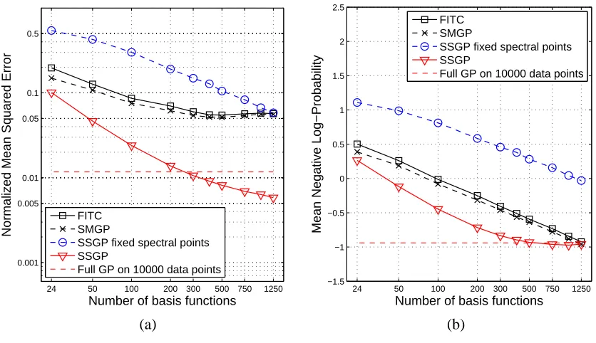
Figure 3: Kin-40k data set. (a) NMSE and (b) MNLP as a function of the number of basis functions.

(10)

10 24 50 74 100 0.04

0.05 0.1

FITC SMGP

10 24 50 74 100

−0.2 −0.15 −0.1 −0.05 0 0.05 0.1 0.15 0.2

FITC SMGP

(a) (b)

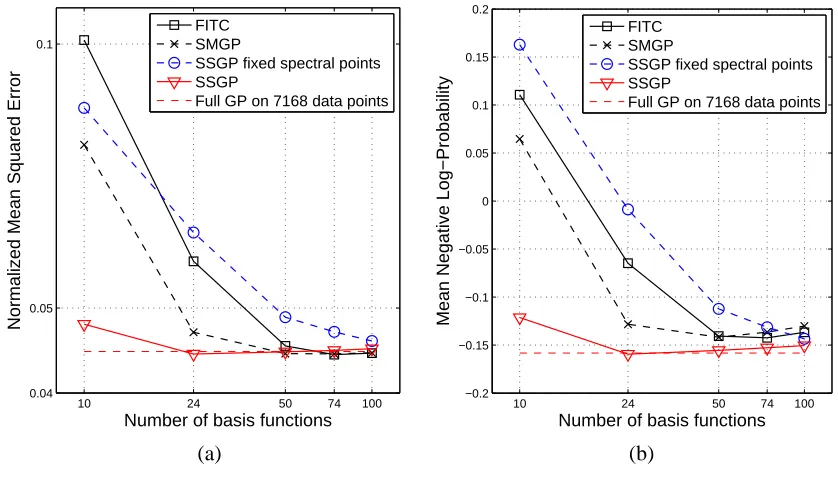
Figure 4: Pumadyn-32nm data set. (a) NMSE and (b) MNLP as a function of the number of basis functions.

Figure 2 compares the predictive posterior distributions of SSGP and FITC for a simple synthetic

data set. The training data is generated by evaluating the sinc function on 100 random inputs x∈

[−1,5]and adding white, zero-mean Gaussian noise of varianceσ2_n=0.052. SSGP is given 20 fixed

spectral points sampled from the spectrum of a squared exponential covariance function, and FITC is given 40 fixed pseudo-inputs sampled uniformly from the range of the training inputs. The rest of the hyperparameters are optimized in both cases by maximizing the marginal likelihood. We plot

the 95% confidence interval for both predictive distributions (mean±two standard deviations), and

draw three samples from the SSGP posterior and one sample from the FITC posterior.

Despite the different nature of the approximations, the figure shows that for an equal number of basis functions both predictive distributions are qualitatively very similar: the uncertainty grows away from the training data. In the following section, we verify empirically that the SSGP is a practical approximation for modelling non-periodic data.

5.2 Performance Evaluation

We will use two quantitative performance measures: the test Normalized Mean Square Error (NMSE) and the test Mean Negative Log Probability (MNLP) , defined as:

NMSE=h(y∗j−µ∗j)

2_i

h(y∗j−y)2i

and MNLP= 1

2

Dy_∗_j−µ_∗_j

σ∗j

2

+logσ2_∗_j+log 2π

E

, (13)

where µ∗j andσ2∗j are, respectively, the predictive mean and variance for test sample j and y∗j is

(11)

the average over test cases byh·i. For all experiments the values reported are averages over ten repetitions.

For each data set we report the performance of five different methods: first, the SSGP algorithm as presented in Section 4.2; second, a version of SSGP where the spectral points are “fixed” to sam-ples from the spectral density of a squared exponential covariance function whose lengthscales are

learned (SSGP fixed spectral points);4 third, the FITC approximation, learning the pseudo-inputs;

fourth, SMGP, trained as described in Walder et al. (2008); and finally as a base line comparison we report the result of a full GP trained on the entire training set. We plot the performance as a function of the number of basis functions. For FITC this is equivalent to the number of pseudo-inputs, whereas for SSGP a spectral point corresponds to two basis functions. The number of basis functions is a good proxy for computational cost.

We consider four data sets of size moderate enough to be tractable by a full GP, but still large enough that there is a motivation for computationally efficient approximations.

The two first data sets are both artificially generated using a robot arm simulator and are highly non-linear and have very low noise. They were both used in Seeger et al. (2003) and Snelson and Ghahramani (2006), but note that their definition of the NMSE measure differs by a factor of 2 from our definition in (13). We follow precisely their preprocessing and use the original splits. The first data set is Kin-40k (8 dimensions, 10000 training and 30000 testing samples) and the results are displayed in Figure 3. For both error measures SSGP outperforms FITC and SMGP by a large margin, and even improves on the performance of the full GP. The SSGP with fixed spectral points is inferior, proving that a greater sparsity vs. accuracy tradeoff can be achieved by optimizing the spectral points.

The Pumadyn-32nm problem (32 dimensions, 7168 training and 1024 testing samples) can be seen as a test of the ARD capabilities of a regression model, since only 4 out of the 32 input dimensions are relevant. Following Snelson and Ghahramani (2006), to avoid getting stuck at an undesirable bad local optimum, lengthscales are initialized from a full GP on a subset of 1024 training data points, for all compared methods. The results are shown in figure 4.

The conclusions are similar as for the Kin-40k data set. SSGP matches the full GP for a surpris-ingly small number of basis functions.

The Pole Telecomm and the Elevators data sets are taken from http://www.liaad.up.pt/

~ltorgo/Regression/DataSets.html. In the Pole Telecomm data set we retain 26 dimensions, removing constants. We use the original split, 10000 data for training and 5000 for testing. Both the inputs and the outputs take a discrete set of values. In particular, the outputs take values between 0 and 100, in multiples of 10. We take into account the output quantization by lower bounding the

value ofσ2_nto the value of the quantization noise, bin2_spacing/12. This lower bounding is applied to

all the compared methods. The effect is to provide a better estimation forσ2_nand therefore, better

MNLP measures, but we have observed that this modification has no noticeable effect on NMSE values. Resulting plots are in Figure 5.

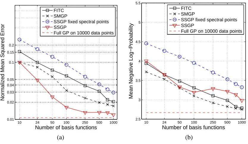
SSGP is superior in terms of NMSE, getting very close to the full GP for more than 200 basis functions. In terms of MNLP, SSGP is between FITC and SMGP for small m, but slightly worse for more than 100 basis functions. This may be an indication that SSGP produces better predictive means than variances. We also see that SSGP with fixed spectral points is uniformly worse.

(12)

10 24 50 100 250 500 1000 0.01

0.02 0.03 0.04 0.05 0.1 0.15 0.2

FITC SMGP

10 24 50 100 250 500 1000

2.5 3 3.5 4 4.5 5 5.5

FITC SMGP

(a) (b)

Figure 5: Pole Telecomm data set. (a) NMSE and (b) MNLP as a function of the number of basis functions.

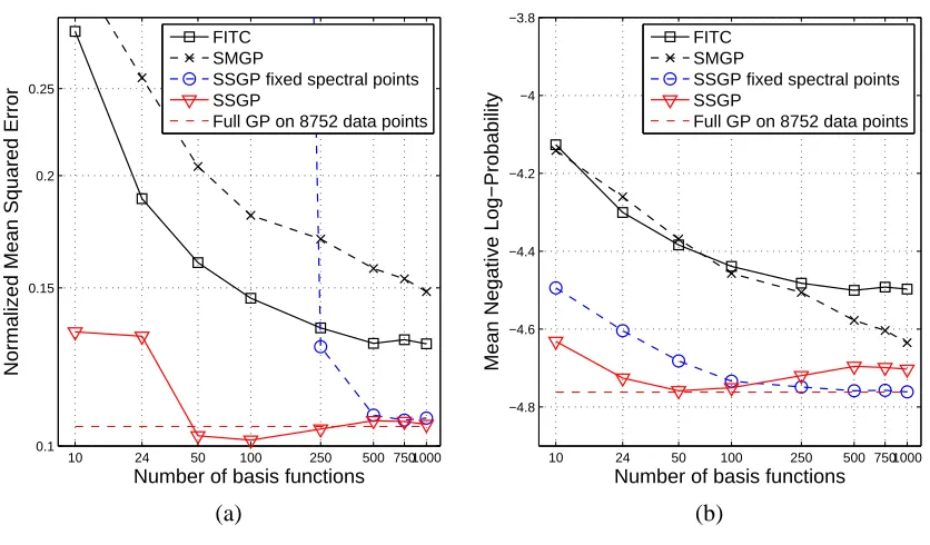
The fourth data set, Elevators, relates to controlling the elevators of an F16 aircraft. After removing some constant inputs the data is 17-dimensional. We use the original split with 8752 data for training and 7847 for testing. Results are displayed in Figure 6. SSGP consistently outperforms FITC and SMGP and gets very close to the full GP using a very low number of basis functions. The large NMSE average errors incurred by SSGP with fixed spectral points for small numbers of basis functions are due to outliers that are present in a small number (about 10 out of 7847) of the test inputs, in some of the 10 repeated runs. The predictive variances for these few points are also big, so their impact on the MNLP score is small. Such an effect has not been observed in any of the other data sets.

5.3 Explicit Phase Representation

(13)

10 24 50 100 250 500 7501000 0.1

0.15 0.2 0.25

FITC SMGP

10 24 50 100 250 500 7501000

−4.8 −4.6 −4.4 −4.2 −4 −3.8

FITC SMGP

(a) (b)

Figure 6: Elevators data set. (a) NMSE and (b) MNLP as a function of the number of basis func-tions.

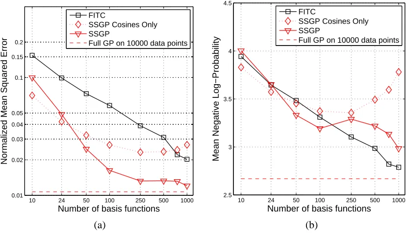
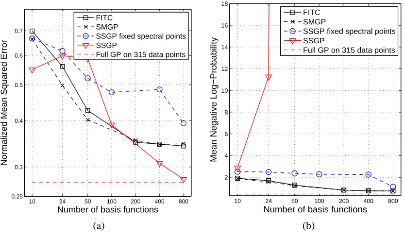
5.4 The Pendulum Data Set

So far we have seen data sets where SSGP consistently outperforms FITC and SMGP, and often approaches the performance of a full GP for quite small numbers of basis functions. In this section we present a counter example, showing that SSGP may occasionally fail, although we suspect that this is the exception rather than the norm.

(14)

10 24 50 100 250 500 1000 0.01

0.02 0.03 0.04 0.05 0.1 0.15 0.2

FITC

SSGP Cosines Only SSGP

10 24 50 100 250 500 1000

2.5 3 3.5 4 4.5

FITC

SSGP Cosines Only SSGP

(a) (b)

Figure 7: Pole Telecomm data set. (a) NMSE and (b) MNLP as a function of the number of basis functions, comparing SSGP with the version with cosines only and explicit phases.

falling in the overfitting trap. We nevertheless think that the SSGP algorithm will often have very good performance, and will be a practically important algorithm, although one must use it with care.

6. Discussion

We have introduced the Sparse Spectrum Gaussian Process (SSGP) algorithm, a novel perspective on sparse GP approximations where rather than the usual sparsity approximation in the spatial do-main, it is the spectrum of the covariance function that is subject to a sparse approximation by means of a discrete set of samples, the spectral points. We have provided a detailed comparison of the computational complexity vs. accuracy tradeoff of SSGP to that of the state of the art GP sparse approximation FITC and its extension SMGP. SSGP shows a dramatic improvement in four commonly used benchmark regression data sets, including the two data sets used for evaluation in the paper where FITC was originally proposed (Snelson and Ghahramani, 2006). However, we found a small data set where SSGP badly fails, with good predictive means but with overconfident predictive variances. This indicates that although SSGP is practically a very appealing algorithm, care must be taken to avoid the occasional risk of overfitting.

(15)

10 24 50 100 200 400 800 0.25

0.3 0.4 0.5 0.6 0.7

FITC SMGP

10 24 50 100 200 400 800

2 4 6 8 10 12 14 16 18

FITC SMGP

(a) (b)

Figure 8: Pendulum data set. (a) NMSE and (b) MNLP as a function of the number of basis func-tions.

typically achieve superior performance, see Figure 3 in Titsias (2009), with some risk of overfitting. Note, that these algorithms don’t generally converge toward the full GP.

An equivalent view of SSGP is as a sparse Bayesian linear combination of pairs of trigonometric basis functions, a sine and a cosine for each spectral point. The weights are integrated out, and at the price of having two basis functions per frequency, the phases are effectively integrated out as well. We have shown that although a representation in terms of a single basis function per frequency and an explicit phase is possible, learning the phases poses an increased risk of overfitting. If the spectral points are sampled from the power spectrum of a stationary GP, then SSGP approximates its covariance function. However, much sparser solutions can be achieved by learning the spectral points, which effectively implies learning the covariance function. The SSGP model is to the best of our knowledge the only sparse GP approximation that induces a stationary covariance function.

SSGP has been presented here as a Gaussian process prior for regression with a tractable like-lihood function from the assumption of Gaussian observation noise. Extending to other types of analytically intractable likelihood functions, such as sigmoid for classification or Laplace for robust regression is possible by using the same approximation techniques as for full GPs. An example is the use of Expectation Propagation in the derivation of generalized FITC (Naish-Guzman and Holden, 2008). Further modifications and extensions of SSGP are discussed in Lázaro-Gredilla (2010).

(16)

investigate more carefully in the future the exact conditions under which these spectacular sparsity vs. accuracy improvements can be expected.

Acknowledgments

This work has been partly supported by an FPU grant (first author) from the Spanish Ministry of Education and CICYT project TEC-2005-00992 (first and last author). Part of this work was developed while the first author was a visitor at the Computational and Biological Learning Lab, Department of Engineering, University of Cambridge.

Appendix A. Details of the Implementation

In practice, to improve numerical accuracy and speed, Equations (7) and (8) should be implemented

using the Cholesky decomposition R=chol(A). Thus the predictive distribution is computed as

E_[_y_∗_{] =} φ₍_x_∗₎⊤_R_\₍_R⊤_\₍Φ_f_y₎₎ V_[_y_∗_{] =} σ2_n₊σ2_n_||_R⊤_\φ₍_x_∗₎_||2_,

and the log evidence as

log p(y|θ) = − 1

2σ2

n

h

||y||2− ||R⊤\(Φfy)||2

i

−1

2

∑

_i log R

2

ii+m log mσ2_n

σ2 0

−n

2log 2πσ

2 n,

where Riirefers to the diagonal elements of R.

References

G. L. Bretthorst. Nonuniform sampling: Bandwidth and aliasing. In Maximum Entropy and

Bayesian Methods, pages 1–28. Kluwer, 2000.

A. B. Carlson. Communication Systems. McGraw-Hill, 3rd edition, 1986.

L. Csató and M. Opper. Sparse online Gaussian processes. Neural Computation, 14(3):641–669, 2002.

M. Lázaro-Gredilla. Sparse Gaussian Processes for Large-Scale Machine Learning. PhD

the-sis, Universidad Carlos III de Madrid, 2010. URL http://www.tsc.uc3m.es/~miguel/

publications.php.

M. Lázaro-Gredilla and A.R. Figueiras-Vidal. Inter-domain Gaussian processes for sparse inference using inducing features. In Advances in Neural Information Processing Systems 22, pages 1087– 1095. MIT Press, 2010.

M. Lázaro-Gredilla, J. Quiñonero-Candela, and A. Figueiras-Vidal. Sparse spectral sampling Gaus-sian processes. Technical report, Microsoft Research, 2007.

(17)

A. Naish-Guzman and S. Holden. The generalized FITC approximation. In Advances in Neural

Information Processing Systems 20, pages 1057–1064. MIT Press, 2008.

J. Quiñonero-Candela and C. E. Rasmussen. A unifying view of sparse approximate Gaussian process regression. Journal of Machine Learning Research, 6:1939–1959, 2005.

J. Quiñonero-Candela, C. E. Rasmussen, and C. K. I. Williams. Approximation methods for Gaus-sian process regression. In L. Bottou, O. Chapelle, D. DeCoste, and J. Weston, editors,

Large-Scale Kernel Machines, pages 203–223. MIT Press, 2007.

A. Rahimi and B. Recht. Random features for large-scale kernel machines. In Advances in Neural

Information Processing Systems 20, pages 1177–1184. MIT Press, Cambridge, MA, 2008.

C. E. Rasmussen and Joaquin Quiñonero-Candela. Healing the relevance vector machine through augmentation. In Proceedings of the 22nd International Conference on Machine Learning, pages 689–696, 2005.

C. E. Rasmussen and C. K. I. Williams. Gaussian Processes for Machine Learning. The MIT Press, 2006.

M. Seeger, C. K. I. Williams, and N. D. Lawrence. Fast forward selection to speed up sparse Gaussian process regression. In Proceedings of the 9th International Workshop on AI Stats, 2003.

A. J. Smola and P. Bartlett. Sparse greedy Gaussian process regression. In Advances in Neural

Information Processing Systems 13, pages 619–625. MIT Press, 2001.

E. Snelson and Z. Ghahramani. Sparse Gaussian processes using pseudo-inputs. In Advances in

Neural Information Processing Systems 18, pages 1259 ˝U–1266. MIT Press, 2006.

M. L. Stein. Interpolation of Spatial Data. Springer Verlag, 1999.

M. K. Titsias. Variational learning of inducing variables in sparse Gaussian processes. In

Proceed-ings of the 12th International Workshop on AI Stats, 2009.

V. Tresp. A Bayesian committee machine. Neural Computation, 12:2719–2741, 2000.

R. Urtasun and T. Darrell. Sparse probabilistic regression for activity-independent human pose inference. In Computer Vision and Pattern Recognition, 2008. CVPR 2008. IEEE Conference on, pages 1–8, 2008.

C. Walder, K. I. Kim, and B. Schölkopf. Sparse multiscale Gaussian process regression. In 25th

International Conference on Machine Learning. ACM Press, New York, 2008.

C. K. I. Williams. Computing with infinite networks. In Advances in Neural Information Processing

Systems 9, pages 1069–1072. MIT Press, 1997.

C. K. I. Williams and M. Seeger. Using the Nyström method to speed up kernel machines. In