Published online March 2, 2015 (http://www.sciencepublishinggroup.com/j/hyd) doi: 10.11648/j.hyd.20150301.11
ISSN: 2330-7609 (Print); ISSN: 2330-7617 (Online)
Spatial Distribution Analysis and Mapping of Groundwater
Quality Parameters for the Sylhet City Corporation (SCC)
Area Using GIS
Gulam Md Munna
*, Numan-Al-Kibriya, Ahmad Hasan Nury, Shriful Islam, Hasina Rahman
Dept. of Civil and Environmental Engineering, Shahjalal University of Science and Technology, Sylhet, Bangladesh
Email address:
[email protected] (G. M. Munna), [email protected] (N. A. Kibriya), [email protected] (A. H. Nury), [email protected] (S. Islam), [email protected] (H. Rahman)
To cite this article:
Gulam Md Munna, Numan-Al-Kibriya, Ahmad Hasan Nury, Shriful Islam, Hasina Rahman. Spatial Distribution Analysis and Mapping of Groundwater Quality Parameters for the Sylhet City Corporation (SCC) Area Using GIS. Hydrology. Vol. 3, No. 1, 2015, pp. 1-10. doi: 10.11648/j.hyd.20150301.11
Abstract:
As Groundwater is a natural source of drinking water, it needs to be monitored regularly and people should be made aware of its quality. The unscientific management and exploration of groundwater resources has always been a serious problem in many cities in Bangladesh. As a result the quality of groundwater has become equally important as of its quantity. The present study is aimed to assess the current condition of groundwater quality and to analyze the spatial distribution of groundwater quality for the Sylhet City Corporation (SCC) area. The groundwater quality parameters were analyzed for 51 samples collected from the existing shallow tube wells from the twelve wards of SCC area. Arc GIS geostatistical analyst extension module was used for exploratory data analysis, semivariogram model selection, cross validation. Experimental semivariogram values are examined to find out the best fitted ordinary kriging (OK) models for eleven water quality parameters: pH, potassium, total hardness, alkalinity, turbidity, calcium, total dissolve solids, sulfate, nitrate, chloride and iron. The values of prediction errors i.e. mean square error (MSE), root mean square error (RMSE), average standard error (ASE), root mean square standardize error (RMSSE) were considered to justify the best fitted model. The interpolated spatial maps of different groundwater parameters shows that iron, alkalinity, total hardness and turbidity are vulnerable to groundwater quality within the study area.Keywords:
Groundwater, Spatial Distribution, GIS, Geostatistics, Semivariogram1. Introduction
As an important element of earth groundwater is required for human health, socioeconomic development and most importantly for ecosystem. In last few decades, there has been a tremendous increase in the demand for the fresh water due to rapid growth of population and their accelerated pace of industrialization [1]. The important of using safe water has become an international issue with the ever increasing of world population which eventually accelerates the water demand. This scares and fragile resource is under the risk of degradation in both quality and quantity in many parts of the world [2]. Large quantities of human and industries waste disposals pose serious threat to this valuable resource. Excessive pumping and unscientific management of aquifers are also responsible for deterioration of water quality. According to the report of WHO 80% of all the diseases in human being are caused by water. Once the groundwater is
groundwater modeling and mapping. GIS is a complete set of computer system for managing geographic data. Before mid nineties GIS was not sufficiently available in terms of technology and application especially for geographic data such as groundwater. But recently GIS technology has accelerated by the growth of computer technology and become an effective tool for managing huge amount of geographical data to solve various spatial problems. Geostatistical approach of GIS is very helpful to analyze the spatial variation of groundwater quality. Geostatistics follows the basic assumption that the properties of earth have some spatial continuity up to a certain lag distance [9]. Geostatistical approach (Kriging) has several advantages over the deterministic methods [10, 11]. The aim of the study is to provide an overview of groundwater condition with respect to different water quality parameters such as: pH, turbidity, calcium, potassium, total hardness, alkalinity, sulfate, Chloride, total dissolve solids, nitrate, Iron. Spatial distribution map of these quality parameters are an important guideline for the region to evaluate the potential threats and water safeness for drinking purpose.
2. Study Area
Sylhet city is located in between 24°51´ and 24°55´ north latitudes and in between 91°50´ and 91°54´ east longitudes, on the northern bank of the River Surma. It experiences a hot, wet and humid tropical climate. The city is within the monsoon climate zone, with annual average highest temperatures of 23°C (Aug-Oct) and average lowest temperature of 7°C (January).
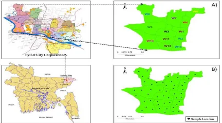
According to Wikipedia [12] nearly 80% of the annual average rainfall of 3,334mm occurs between May and September. Sylhet City Corporation consists of 27 wards and 278 mahallas, it is a small city with an area of 26.50 square km. The present population is nearly about 500,000 [12]. Out of 27 wards, twelve wards are selected for the present study, which mainly covers the half part of city as shown in Figure 1a.The Sylhet City Corporation is capable of supplying a maximum of 21,000 cubic meters of water every day against the demand for 48,000 cubic meters per day. But the city corporation has now actually been supplying between 16,000 to 18,000 cubic meters every day.
Figure 1. a) Study Area. b) Location of Sampling Points
The supply water situation has also worsened because of frequent power outages that happen for about 8 to 10 times a day, mostly during peak hours. The city corporation has more than 10,000 water subscribers. At present city corporation can meet up to 50% of the demand of the city dwellers, the remaining 50% of the demand is met from HTW (DPHE), pond and river water. The primary source of water supply in Sylhet City is mainly from ground water available in the shallow and deep aquifers extracted through (power-operated) deep tube wells. Despite this problem, regular monitoring of water quality has not been conducted.
3. Materials and Methods
3.1. Lab Analysis
Chloride, Total Dissolve Solids (TDS), Nitrate, Iron using Standard Procedures [13]. The sampling locations were obtained using a global positioning system (GPS) receiver. Figure 1b shows the location of the sampling points. The specific Methods of estimation of different Water Quality Parameters are given below in Table 1.
Table 1. Specific methods for estimating different Physico-chemical Parameters
Serial No Groundwater Parameters Methods
1 pH Digital pH Meter 2 Turbidity Nephelometer 3 Calcium EDTA titration 4 Potassium Spectrophotometer 5 Total Hardness EDTA titration 6 Alkalinity Titration Method 7 Sulfate Spectrophotometer 8 Chloride Mohr method 9 Total Dissolve Solids Gravimetric Method 10 Nitrate Spectrophotometer 11 Iron Spectrophotometer
3.2. Geo-Statistical Analysis
Kriging technique has been used for spatial variation analysis as it provides an unbiased prediction with minimum variance and interpolation errors. Such values can be mapped to generate error surfaces which inform about the reliability of the estimation [14]. Kriging involve the following steps:
First step: To check data consistency, removing outliers, statistical distribution, exploratory data analysis needs to be performed. Kriging methods work best for normally distributed data [14]. If the data are not normally distributed, they need to be transformed into normally distributed data using the transformation methods. The most common transformation type is logarithmic because of its simplicity. The log transformation is as follows
Y(s) = ln (Z(s)) (1)
For Z(s) > 0Where Z(s) is observed data, Y(s) is transform normal data and ln is the natural logarithm.
Second step: Semivariogram is estimated to determine the spatial correlation or dependence from the observed data. semivariogram is estimated from half the expected squared difference between paired data values z(x) and z(x + h) to the distance lag h, by which locations are separated.
ℎ = − + ℎ 2 (2)
Where Z (Xi) is the value of the variable Z at location of Xi, h is the lag distance, and N (h) is the number of pairs of sample points separated by h.
ℎ = ∑ – + ℎ 2 (3)
For irregular sampling, it is rare for the distance between the sample pairs to be exactly equal to h. After estimating the semivariogram, the values are fitted through theoretical models: circular, Gaussian, spherical, exponential. The best fitted model will be used for further prediction. Ordinary
kriging (OK) has been used in the present study for its simplicity and accuracy. OK uses a probability model where the bias and the error variance can both be calculated ensuring the average error for the model is close to zero and at the same time minimize the error variance.
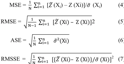
Third step: Four theoretical models (circular, Gaussian, spherical, exponential) were checked for every water quality parameters on the basis of cross validation test to select the best one. Cross-validation uses all the data to estimate the trend and autocorrelation models by removing each data location one at a time and predicts the associated data value [14]. This validation compares the predictive values to the observed values and obtains useful information about the quality of OK model. Cross validation is performed automatically in the last step of Arc GIS geostatistical wizard. The values of mean standardize error (MSE), root mean error (RMSE), average standard error (ASE) and root mean square standardized error (RMSSE) were the determining factors of selecting best model. Each kriging techniques provide the kriging variance that estimate the variability of prediction for known values. The kriging variance must be calculated for each model to avoid the conflict among errors. MSE is 0 for an accurate model. To assess the prediction errors correctly RMSE must close to the ASE. RMSSE should close to one. Underestimated predictions have RMSSE greater than, one; likewise overestimated predictions have RMSSE less that one. The various errors are defined by the equations (4)-(7):
MSE = ∑ [ (Xi) – Z (Xi)]/ (Xi) (4)
RMSE =
! ∑ Xi – Z Xi 2 (5)
ASE = ∑ ² Xi (6)
RMSSE = ∑ { Xi – Z Xi }/ Xi 2 (7)
Where ² (Xi) is the Kriging Variance for location Xi.Finally the thematic maps of each groundwater quality parameters were generated using ordinary kriging.
4. Result and Discussion
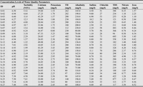
The water quality parameters are assessed by comparing the test results with both Bangladesh Drinking Water Standard (ECR, 1997)[16] and World Health Organization (WHO)[15] guidelines for drinking water quality (WHO, 2006).The analyzed concentrations of different water quality parameters are presented in the table 2. The analysis shows that all the parameters are found to be within the desirable limit except Iron & Turbidity. Table 3 shows the generalized information of the analyzed samples with respect to maximum, minimum and standard values as well as statistical parameters.
S-36, S-42, S-45). These samples have pH below 6.5 indicating acidic water. One of the main objectives to control pH is to generate water that minimizes corrosion or incrustation. The results from increased pH can cause damage to the water supply systems with other interacting parameters such as dissolved solids, dissolved gases, hardness, alkalinity and temperature. There is also a decrease in the efficiency of chlorine disinfection with the increase of pH levels.
Turbidity levels of groundwater ranged from 0.96 NTU to 13.6 NTU. Out of 51 groundwater samples analyzed, the turbidity levels in 46 samples were found to be within the standard limit (10 NTU) by both WHO and BDWS recommended limits. In the remaining 5 samples (S-03, S-04, S-06, S-07, S-31) the turbidity exceeded the standard limit.
Calcium concentration in groundwater ranged from 10.4 mg/l to 67.33 mg/l, this implies that the concentrations of calcium for all the groundwater samples are within the desirable limit (75 mg/l) by WHO and BDWS.
Potassium concentrations in groundwater are also within the desirable limit 12 mg/l as recommended by WHO and BDWS. Potassium limit ranges from 0.88 mg/l to 4.27 mg/l within the study area.
Total Hardness in the study area ranges from 36 mg/l to 402 mg/l where Water hardness is the traditional measure of the capacity of water to react with soap, hard water requiring considerably more soap to produce lather. Hard water often produces a noticeable deposit of precipitates (e.g. insoluble metals, soaps or salts) in containers, including “bathtub rings”.
Alkalinity of the samples are in the range of 50-230 mg/l indicating all the samples are within the BDWS standard 500 mg/l. Maximum concentration is found in groundwater sample collected from pathantula 230 mg/l. Most of the water samples have alkalinity greater than 100 mg/l as recommended by WHO. High alkalinity level indicates resistance to acidification of groundwater.
Sulfate concentration in collected groundwater samples is ranges from 0.1 mg/l to 11.1 mg/l as in the permissible limit of 250 mg/l recommended by WHO and 400 mg/l recommended by BDWS. Maximum concentration is found in groundwater sample collected from Housing estate 11.1 mg/l and Minimum concentration is found in groundwater sample collected from Dargamahalla 0.1 mg/l.
Chloride concentration in collected groundwater samples ranges from 22 mg/l to 80 mg/l as in the permissible limit of 250 mg/l recommended by WHO and 150-600 mg/l recommended by BDWS. Maximum concentration is found in groundwater sample collected from Pirmahalla 80 mg/l and Minimum concentration is found in groundwater sample collected from Kuarpar 22 mg/l.
Total dissolved solids concentration ranges from 94 -877 mg/l well below the permissible limit 1000 mg/l recommended by both WHO and BDWS. The term total dissolved solids refer mainly to the inorganic substances that are dissolved in water. The effects of TDS on drinking water quality depend on the level of its individual components; excessive harness, taste, mineral deposition and corrosion are common properties in highly mineralized water.
Table 2. Concentrations of Groundwater quality Parameters
Concentration Levels of Water Quality Parameters
ID pH Turbidity
(NTU) Calcium (mg/l) Potassium (mg/l) TH (mg/l) Alkalinity (mg/l) Sulfate (mg/l) Chloride (mg/l) TDS (mg/l) Nitrate (mg/l) Iron (mg/l)
Concentration Levels of Water Quality Parameters
ID pH Turbidity
(NTU) Calcium (mg/l) Potassium (mg/l) TH (mg/l) Alkalinity (mg/l) Sulfate (mg/l) Chloride (mg/l) TDS (mg/l) Nitrate (mg/l) Iron (mg/l)
S-28 7.62 8.75 10.40 2.61 70 185.0 1.10 58 229 2.29 0.47 S-29 7.58 1.91 19.00 1.98 78 168.0 0.40 44 170 3.25 0.48 S-30 7.83 2.49 18.00 1.33 86 165.0 1.00 43 214 3.40 1.05 S-31 7.55 11.5 20.00 4.27 116 223.0 1.10 64 315 1.25 0.49 S-32 6.70 1.95 14.00 3.33 52 160.0 0.80 43 275 2.23 0.99 S-33 6.09 3.99 12.00 2.13 52 180.0 3.20 53 153 1.75 1.43 S-34 6.83 3.04 18.00 2.25 125 170.0 2.40 47 215 0.87 0.87 S-35 6.79 1.12 17.64 2.17 69 186.0 1.10 34 200 0.20 0.34 S-36 5.92 1.30 40.08 2.23 140 106.0 3.30 42 116 0.87 2.58 S-37 6.87 1.34 20.07 2.01 140 175.0 0.90 54 185 0.50 0.57 S-38 6.55 2.38 24.05 1.87 160 200.0 0.60 38 211 0.20 0.44 S-39 6.85 1.56 43.29 1.18 220 190.0 0.70 31 224 0.20 0.91 S-40 6.70 0.96 26.03 1.05 240 154.0 1.60 24 195 0.10 0.58 S-41 6.85 2.35 24.05 1.89 140 112.0 1.60 37 170 0.30 0.90 S-42 6.45 2.42 32.06 1.17 120 108.0 1.70 22 172 0.40 2.01 S-43 6.78 8.99 19.24 2.15 222 74.00 0.70 26 101 1.15 0.76 S-44 6.70 1.73 24.00 2.20 132 125.0 1.10 48 262 2.30 0.50 S-45 6.44 2.89 17.64 2.14 190 50.00 2.50 73 206 4.70 0.60 S-46 6.76 1.26 56.11 1.48 200 72.00 3.80 56 350 1.72 0.65 S-47 6.65 6.93 16.03 2.24 160 114.0 1.80 37 139 2.25 1.43 S-48 6.93 3.97 22.08 3.48 260 115.0 3.40 54 211 3.05 0.56 S-49 6.81 4.36 16.03 1.15 240 90.00 5.80 42 227 1.20 0.41 S-50 6.73 4.02 24.05 2.75 214 130.0 2.90 29 186 0.50 1.36 S-51 6.70 5.99 19.24 3.25 236 104.0 2.10 27 167 0.20 0.85
(Continued……..)
Table 3. Generalize information of Dataset with Standards
Parameter Mean Median Standard deviation Skewnees Kurtosis N Min Max WHO BD standard
pH 6.872 6.880 0.363 0.265 4.046 51 5.93 7.830 6.5-8.5 6.5-8.5 Turbidity 4.611 3.390 3.294 1.070 3.219
51 0.96 13.60 5 10 Turbidity** 1.285 1.221 0.712 0.0831 2.005
Calcium 25.29 22.00 11.31 1.583 5.828
51 10.4 67.33 75 75 Calcium** 3.149 3.095 0.395 0.4938 3.025
Potassium 2.311 2.200 0.780 0.388 2.569 51 0.88 4.270 - 12 TH 174.1 180.0 81.29 0.292 2.628 51 36.0 402.0 - 200-500 Alkalinity 136.9 143.0 48.09 -0.028 1.935 51 50.0 230.0 100 500 Sulfate 3.078 1.800 3.069 1.205 3.255
51 0.10 11.10 250 400 Sulfate** 0.588 0.588 1.120 -0.216 2.437
Chloride 42.86 42.00 14.99 0.479 2.452 51 22.0 80.00 250 150-600 TDS 245.7 211.0 141.8 2.411 10.32
51 94.0 877.0 1000 1000 TDS** 5.387 5.352 0.465 0.629 3.598
Nitrate 1.738 1.250 1.494 2.982 0.955
51 0.10 5.500 50 10 Nitrate** 0.108 0.223 1.041 -0.353 2.153
Iron 0.963 0.790 0.645 1.639 5.248
51 0.24 3.050 0.3 0.3-1.0 Iron** -0.215 -0.235 0.584 0.403 2.670
** Log Transformation used parameters
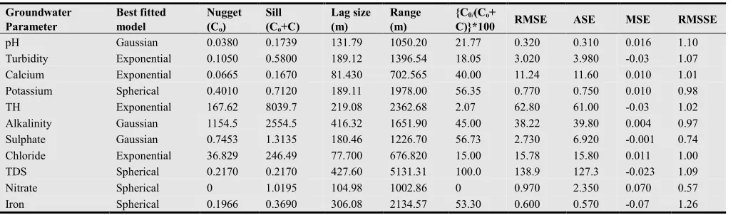
Table 4. Characteristics parameters of selected semivariogram models
Groundwater Parameter
Best fitted model
Nugget (Co)
Sill (Co+C)
Lag size (m)
Range (m)
{C0/(Co+
C)}*100 RMSE ASE MSE RMSSE
In the groundwater of SCC Nitrate level varies from 0.1 mg/l to 5.5 mg/l which complies with the permissible limit of 10 mg/l as per BDWS standards and 50 mg/l as per WHO standards. Iron concentration in the groundwater samples varies from 0.24 to 3.05 mg/L which exceeds the permissible limit of 0.3-1.0 mg/L as per BDWS and 0.3 mg/L as per WHO Standards.
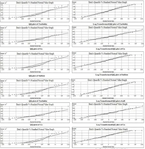
The groundwater samples exhibited high Iron contamination which is an indication of the presence of ferrous salts that precipitate as insoluble ferric hydroxide and settles out as rusty silt. The exploratory spatial data analysis was performed to check the distribution pattern of the dataset. The normal QQ plots were plotted for each parameter as shown in figure 2. pH, potassium, Alkalinity and Chloride show normal distribution as all the points in each figure fall above or below the 45 degree reference line and Turbidity, Calcium, TDS, Sulfate, Nitrate and Iron do not show normal distribution as all the pints are more or less deviated from the 45 degree reference line-Figure 2. Log transformation was used for these parameters to transform into the normal distribution so that all the points for these parameters eventually fall on the 45 degree reference line. The statistical information table 3 shows, that normally distributed parameters have similar value of median and mean with positive skewed values close to zero.
On the other hand before transformation for parameters Turbidity, Calcium, TDS, Sulfate, Nitrate and Iron have different median and mean with high skewed values which do not fulfill the criteria of normal distribution. So log transformation was performed for these parameters figure
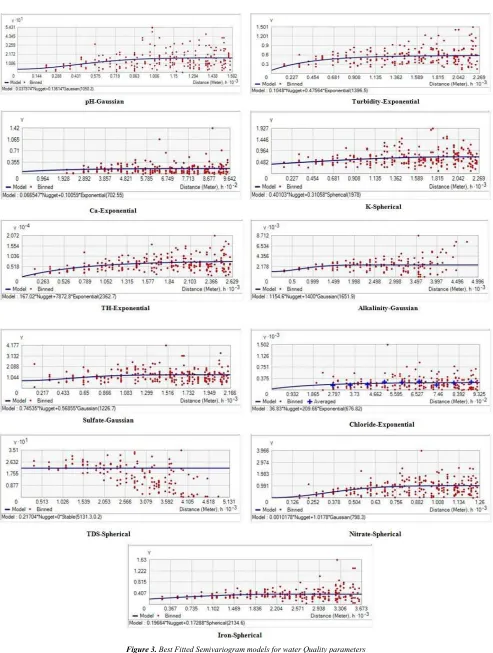
2.Semivariogram model fitting was conducted using ordinary kriging and the best fitted models for water quality parameters are shown in figure 3. Each of the figures represents lag distance vs semivariance values contributing a model with its different quantitative components. The blue line indicates the theoretical model that has been selected for prediction as most of the semivariance values are close to that line as shown for each quality parameters. Table 3 shows the characteristics parameters i.e. sill, nugget, range, lag size and prediction error for the reliance of selected models. The best fitted model for the prediction of pH, Turbidity, Calcium, Potassium, Total Hardness (TH), Alkalinity, Sulfate, Chloride, Total Dissolve Solids (TDS), Nitrate, Iron were Gaussian, Exponential, Exponential, Spherical, Exponential, Gaussian, Gaussian, Exponential, spherical, spherical, spherical respectively. Table 3 shows that pH, turbidity, TH, Cl. NO3 have strong spatial
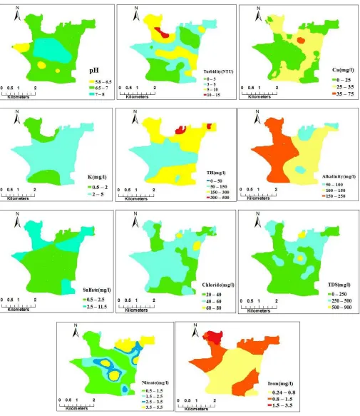
Figure 4. Spatial Distribution Map of Groundwater Quality Parameters
The spatial distribution of different groundwater quality parameters were carried out through GIS geo-statistical Technique using ordinary Kriging. The spatial distribution Map of pH, Turbidity, Calcium, Potassium, Total Hardness (TH), Alkalinity, Sulfate, Chloride, Total Dissolve Solids (TDS), Nitrate, Iron are shown in figure 4. The maps clearly show the concentration variation of water quality parameters
within the region. Turbidity, total Hardness, alkalinity and iron are the key parameters which control the quality of water in the SCC region.
5. Conclusion
done in Sylhet City Corporation area with GIS geostatistical techniques. As sampling from every possible location is not economical, the interpolation technique (ordinary Kriging) played a vital role to predict the values from unmeasured location. Lab analysis of water quality parameters (table 2) showed that 100% of the samples concentration for pH, Ca, potassium, TH, alkalinity sulfate, chloride, TDS and nitrate are well below the Standard recommended by BDWS. Besides thematic maps of these mentioned quality parameters showed a strong prediction results within the standard of BDWS for overall area. On the contrary 34% of collected samples exceed the concentration value of 1.0 for iron as recommended by BDWS which clearly reveals certain levels of iron treatment are necessary at some regions (red and light red) of the area to use the best quality of water. As for turbidity the exceeding concentration is around 10% to BDWS standard which can be acceptable. The study illustrates the use of geostatistical technique for investigating spatial variation of water quality which is more effective effort toward groundwater management system. The thematic maps of groundwater quality parameters will be beneficial to the city authority for effective management and monitoring of groundwater. Other geostatistical techniques (IDW, EBK) may be considered to evaluate the variation of result. The study was only conducted for the month of January, which is a comparatively dry season in Bangladesh. Result may vary during the months of monsoons and heavy rainfall.
References
[1] A. N. Amadi, P.I. Olasehinde, J. Yisa, (2010). Characterization of Groundwater Chemistry in the Coastal plain-sand Aquifer of Owerri using Factor Analysis. Int. J. Phys. Sci., 5(8): 1306-1314.
[2] K.Ambiga, Dr. R. Anna Durai, (2013). Use of Geographical Information System and Water Quality Index to assess Groundwater Quality in and around Ranipet area, Vellor District, Tamilnadu. Int. J. Adv. Engg. Res. Studies /II/IV/73-80.
[3] Mufid al-hadithi, (2012). Application of water quality index to assess suitability of groundwater quality for drinking purposes in Ratmao –PathriRao watershed, Haridwar District, India. Am. J. Sci. Ind. Res., 3(6): 395-402.
[4] Mridha, M.A.K., Rashid, M.H. and Talukder, K.H., (1996). Quality of groundwater for irrigation in Natore, district, Bangladesh. Journal of Agricultural Research, 21, 15-30. [5] Shahid, S., Chen, X. and Hazarika, M.K., (2006). Evaluation of
groundwater quality for irrigation in Bangladesh using geographic information system. Journal of Hydrology and Hydromechanics, 54(1), 3-14.
[6] Sajal Kumar Adhikary, Md. Manjur-A-Elahi, A.M. IqbalHossain, (2012). Assessment of shallow groundwater quality from six wards of Khulna City Corporation, Bangladesh. Int. Journal of Applied Sciences and Engineering Research, Vol. 1, Issue 3.
[7] UNESCO/WHO/UNEP (1996). Water Quality Assessments—a guide to use of biota, sediments and water in environmental monitoring, 2nd edn. In: Chapman D (ed) Chapman & Hall Publishers. ISBN 0419215905(HB) 0419 216006(PB)
[8] P. Balakrishnan1, Abdul Saleem, N. D. Mallikarjun, (2011). Groundwater quality mapping using geographic information system (GIS): A case study of Gulbarga City, Karnataka, India. Afr. J. Environ. Sci. Technol. Vol. 5(12), pp. 1069-1084. [9] Gorai AK, Kumar S (2013) Spatial Distribution Analysis of
Groundwater Quality Index Using GIS: A Case Study of Ranchi Municipal Corporation (RMC) Area. GeoinforGeostat: An Overview 1:2.
[10] Isaaks EH, Srivastava RH (1989) An Introduction to Applied Geostatistics. Oxford University Press, New York.
[11] Goovaerts P (1997) Geostatistics for natural recources evaluation. Geostatistics for natural resources evaluation. Oxford University Press, Applied Geostatistics Series. [12] Wikipedia: http://en.wikipedia.org/wiki/Sylhet
[13] APHA, (2005). “Standard methods for the examination of water and wastewater”. American Public Health Association, Washington D.C
[14] ESRI, (2003). ArcGIS. Environmental Systems Research Institute (ESRI), available online: http://www.ESRI.com/ [15] WHO (World Health Organization) (2006). Guidelines for
drinking water quality, World Health Organization, Geneva, Switzerland.