Multi-class Discriminant Kernel Learning via Convex Programming

Multi-class Discriminant Kernel Learning via Convex Programming

Jieping Ye [email protected]

Shuiwang Ji [email protected]

Jianhui Chen [email protected]

Department of Computer Science and Engineering Center for Evolutionary Functional Genomics The Biodesign Institute

Arizona State University Tempe, AZ 85287, USA

Editor: Isabelle Guyon and Amir Saffari

Abstract

Regularized kernel discriminant analysis (RKDA) performs linear discriminant analysis in the fea-ture space via the kernel trick. Its performance depends on the selection of kernels. In this paper, we consider the problem of multiple kernel learning (MKL) for RKDA, in which the optimal kernel matrix is obtained as a linear combination of pre-specified kernel matrices. We show that the kernel learning problem in RKDA can be formulated as convex programs. First, we show that this problem can be formulated as a semidefinite program (SDP). Based on the equivalence relationship between RKDA and least square problems in the binary-class case, we propose a convex quadratically con-strained quadratic programming (QCQP) formulation for kernel learning in RKDA. A semi-infinite linear programming (SILP) formulation is derived to further improve the efficiency. We extend these formulations to the multi-class case based on a key result established in this paper. That is, the multi-class RKDA kernel learning problem can be decomposed into a set of binary-class kernel learning problems which are constrained to share a common kernel. Based on this decomposition property, SDP formulations are proposed for the multi-class case. Furthermore, it leads naturally to QCQP and SILP formulations. As the performance of RKDA depends on the regularization pa-rameter, we show that this parameter can also be optimized in a joint framework with the kernel. Extensive experiments have been conducted and analyzed, and connections to other algorithms are discussed.

Keywords: model selection, kernel discriminant analysis, semidefinite programming, quadrati-cally constrained quadratic programming, semi-infinite linear programming

1. Introduction

function implicitly defines the nonlinear mapping to the feature space, and expensive computations in the high-dimensional feature space can be avoided by evaluating the kernel function. Thus, one of the central issues in kernel methods is the selection of kernels.

To automate kernel-based learning algorithms, it is desirable to integrate the tuning of kernels into the learning process. This problem has been addressed from different perspectives recently. Lanckriet et al. (2004b) pioneered the work of multiple kernel learning (MKL) in which the optimal kernel matrix is obtained as a linear combination of pre-specified kernel matrices. It was shown (Lanckriet et al., 2004b) that the coefficients in MKL can be determined by solving convex programs in the case of support vector machines (SVM) (Vapnik, 1998; Cristianini and Taylor, 2000). This MKL problem was formulated as support kernel machines (SKM) in Bach et al. (2004), and the sequential minimal optimization (SMO) algorithm (Platt, 1999) was proposed to solve it. Recently, this SKM was reformulated as semi-infinite linear program (SILP) which was shown to be scalable to large data sets and a large number of kernels (Sonnenburg et al., 2006; Rakotomamonjy et al., 2007). Micchelli and Pontil (2005, 2007) studied the problem of finding an optimal kernel from a prescribed convex set of kernels by regularization. To deal with problems with structured output, MKL for joint feature map was proposed in Zien and Ong (2007). While most existing work focuses on learning kernels for SVM, Fung et al. (2004) proposed to learn kernels for discriminant analysis. Based on ideas from MKL, this problem was reformulated as SDP in Kim et al. (2006). In general, approaches based on learning linear combination of kernel matrices offer the additional advantage of facilitating heterogeneous data integration from multiple sources. Such formulations have been applied to combine various biological data, for example, amino acid sequences, hydropathy profiles, and gene expression data, for enhanced biological inference (Lanckriet et al., 2004a).

multi-class SDP formulation. Finally, we propose to optimize the regularization parameter along with the kernels in a joint framework. This joint optimization framework is derived from and similar to the work in De Bie et al. (2003); Lanckriet et al. (2004b).

The key contributions of this paper can be highlighted as follows:

• We propose a simplified SDP formulation for the RKDA kernel learning problem in the binary-class case. Based on this simplified form and the equivalence relationship between RKDA and least square problems in the binary-class case, we derive QCQP and SILP formu-lations for this problem.

• We show that the multi-class RKDA kernel learning problem can be decomposed into k binary-class kernel learning problems where k is the number of classes. This leads to two (exact and approximate) SDP formulations in the multi-class case. Based on this decomposi-tion property, we show that the QCQP and SILP formuladecomposi-tions for binary-class problems can be extended naturally to the multi-class case.

• We show that all the proposed formulations can be recast to optimize the regularization param-eter simultaneously. This joint learning framework further automates the learning algorithms.

• We conduct extensive experiments using a collection of benchmark data sets to compare sev-eral relevant algorithms under a unified experimental setup. To demonstrate the effectiveness of the proposed formulations for heterogeneous data integration, we apply these formulations to combine multiple data sources derived from gene expression pattern images (Tomancak et al., 2002).

The rest of this paper is organized as follows: We derive the SDP, QCQP, and SILP formulations for the binary-class case in Section 2. Section 3 extends these formulations to the multi-class case. The joint optimization of regularization parameter is presented in Section 4. Section 5 presents the experimental evaluation, and this paper concludes with discussion and conclusion in Section 6.

Notation

x_∈IRn denotes an n-dimensional vector. Similarly, A_∈IRm×n denotes a matrix with m rows and n columns. I is used to denote the identity matrix of an appropriate dimension and emdenotes

the vector of all ones of length m. For a square symmetric matrix S, S0 means it is positive semidefinite. We also use the short-hand x_≥0 to denote that each component of the vector x is non-negative.

2. Convex Formulations for Binary-class Problems

We use

X

to denote the input or instance space, which is a subspace of IRd, and

Y

=_{−1,+1_}to denote the output or class label set. An input-output pair(x,y), where x∈

X

and y∈

Y

, is called an example. An example is called positive (negative) if its class label is+1(₋1). We assume that the examples are drawn randomly and independently from a fixed, but unknown, underlying probability distribution over

X

_×

Y

.

matrix G∈IRm×m, defined by Gi j =K(xi,xj) is positive semidefinite. Any kernel function K

im-plicitly maps the input set

X

to a high-dimensional (possibly infinite) Hilbert space

H

K equipped

with the inner product(_·,_·)_HK through a mappingφKfrom

X

to

H

K:

K(x,z) = (φK(x),φK(z))_HK.

In kernel-based classification, the algorithms learn a classifier f :

X

_{→ {−}1,+1_}whose decision boundary between the two classes is affine in the feature space

H

K:

f(x) =sgn(wTφK(x) +b),

where w_∈

H

K is the vector of feature weights, b∈IR is the intercept, and sgn(u) = +1, if u>0,

and₋1 otherwise.

Let_{x+₁,_···,x+_m+}and_{x−₁,_···,x−_m

−}denote the collections of data points from the positive and

negative classes, respectively. The total number of data points in the training set is m=m++m₋. For a given kernel function K, the basic idea of RKDA in the binary-class case is to find a direction in the feature space

H

K onto which the projections of the two sets{φK(x+i )}

m+

i=1 and{φK(x−i )} m−

i=1 are well separated. Define the centroids of the two classes as follows:

µ+_K = 1

m+

m+

∑

i=1

φK(x+_i ),

µ−_K = 1

m₋

m−

∑

i=1

φK(x−_i ),

and the two sample class covariance matrices as follows:

S_K+= 1

m+

m+

∑

i=1

(φK(x+_i )₋µ+_K)(φK(x+_i )₋µ+_K)T,

S−_K = 1

m₋

m−

∑

i=1

(φK(x−_i )₋µ−_K)(φK(x−_i )₋µ−_K)T.

Specifically, in RKDA the separation between the two classes is measured by the ratio of the vari-ance(wT(µ+_K−µ−_K))2 _{between the classes to the variance w}T _m+/mS+

K+m−/mS−K

w within the classes. Thus, RKDA maximizes the following objective function:

F1(w,K) =

(wT(µ+_K−µ−_K))2

wT _m

+/mS+K+m−/mSK−+λI

w, (1)

whereλ>0 is the regularization parameter. The optimal weight vector

w∗_≡argmax

w {

F1(w,K)}

that maximizes the objective function in Equation (1) for a fixed kernel function K and a fixed regularization parameterλis given by

w∗= (m+/mS+K+m−/mS−K+λI)−

1_(µ+

The maximum value

F₁∗(K)_≡max

w {F1(w,K)}

of the objective function in Equation (1) achieved by the optimal weight vector w∗is given by

F₁∗(K) = (µ+_K−µ−_K)T _m

+/mSK++m−/mS−K+λI

−1

(µ+_K−µ−_K). (2)

It follows from the Representer Theorem (Sch ¨olkopf and Smola, 2002) that the optimal weight vector in RKDA is in the span of the images of the training points in the feature space. In other words, there exists a vector

α∗_{= [α}+ 1,···,α

+

m+,α −

1,···,α−m−]

T

∈IRm

such that

w∗= m+

∑

i=1

α+

i φK(x+i ) + m−

∑

i=1

α−

i φK(x−i ) =φK(X)α∗,

whereφK(X)is the data matrix in the feature space given by

φK(X) =φK

(x+₁),_···,φK(x+_m+),φK(x−₁),_···,φK(x−_m−) .

The optimal vectorα∗is given by Kim et al. (2006) as

α∗₌1

λ(I−J(λI+JGJ)−1JG)a,

where I is the identity matrix, a is an m-dimensional vector given by

a= [1/m+,···,1/m+,−1/m−,···,−1/m−]T ∈IRm, (3)

the matrix J is defined as:

J=

1 √_m

+(I− 1

m+em+e

T

m+) 0

0 √1_m

−(I−

1

m₋em−eTm−)

! ,

G is restricted to be a linear combination of the p given kernel matrices G1,_···,Gpas

G_∈

G

=

(

G=

p

∑

i=1

θiGi

p

∑

i=1

θi=1, θi_≥0 _∀i )

,

and em+and em−are vectors of all ones of length m

+_{and m}−_{, respectively.} The optimal value F₁∗(K)in Equation (2) is thus given by

F₁∗(K) = (µ+_K−µ−_K)T m+/mS+K+m−/mS−K+λI

−1

(µ+_K−µ−_K) = (µ+_K−µ−_K)Tw∗= (µ+_K−µ_K−)TφK(X)α∗=aTφK(X)TφK(X)α∗

= 1

λaTG(I−J(λI+JGJ)−1JG)a. (4)

(Vandenberghe and Boyd, 1996; Boyd and Vandenberghe, 2004). General-purpose optimization packages such as SeDuMi (Sturm, 1999) use the interior-point methods (Nesterov and Nemirovskii, 1994) to solve SDP. However, for problems of moderate size in machine learning, this overhead of optimal kernel learning is large, and its computation time can easily exceed that of the learning algorithm itself.

We propose a new SDP formulation for this problem in the next subsection. The proposed SDP formulation has a simplified form. Experimental results presented in Section 5 show that the proposed formulation is comparable to the one in Kim et al. (2006). More importantly, this simplified formulation lays the foundation for the extensions to multi-class problems in Section 3 and the joint optimization of regularization parameter in Section 4.

2.1 Simplified SDP Formulation

In the rest of this paper, we work on the centered version of kernel matrices. This is equivalent to centering the data as preprocessed in linear discriminant analysis (LDA) and principal component analysis (PCA). More precisely, given a set of p kernel matrices G1,_···,Gp, the proposed algorithms

learn an optimal kernel matrix ˜G_∈

G

˜, where

˜

G

=

( ˜

G=

p

∑

i=1

θi_G˜_i

p

∑

i=1

θiri=1, θi≥0

) ,

˜

Gi=PGiP, ri=trace(G˜i), and P∈IRm×mis the centering matrix defined as

P=I₋ 1 meme

T

m, (5)

and emis the vector of all ones of size m.

Consider the maximization of the following objective function:

F2(w,K) =

(wT(µ+_K−µ−_K))2

wT(ΣK₊λ_I)w , (6)

whereΣKis defined as follows:

ΣK = m+S+K+m−S−K+

m+m−

m (µ

+

K−µ−K)(µ

+

K−µ−K) T

= m+

∑

i=1

(φK(x+_i )₋µK)(φK(x+_i )₋µK)T+ m−

∑

i=1

(φK(x−_i )₋µK)(φK(x−_i )₋µK)T

= φK(X)PφK(X)T, (7)

P is defined in Equation (5), and

µK=

1 m

m+

∑

i=1

φK(x+_i ) + m−

∑

i=1

φK(x−_i )

!

Theorem 2.1 Given a set of p centered kernel matrices ˜G1,_···,_G˜_{p, the optimal kernel matrix ˜G∈} ˜

G

that maximizes the objective function in Equation (6) can be found by solving the following semidefinite programming problem:

min

θ,t t (8)

subject to

I+1

λ∑ip=1θiG˜i a

aT t

0,

θ≥0,

θT_r=1,

where a is defined in Equation (3),θ= [θ1,···,θp]T, and r=

trace(G1˜ ),_···,trace(G˜p)T .

Proof The optimal weight vector

w∗_≡argmax

w {

F2(w,K)_}

is given by

w∗= (ΣK+λI)−1_(µ+

K−µ−K).

The maximum value of the objective function in Equation (6) achieved by w∗is given by

F₂∗(K)_≡F2(w∗,K) = (µ+K−µ−K)T(ΣK+λI)−1(µ+K−µ−K).

It follows from Appendix A that

w∗= 1 λφK(X)

I₋P(λI+PGP)−1PG

a,

and

F₂∗(K) = (µ+_K−µ−_K)T_w∗_=aT_φK(X)T_w∗

= 1

λaT

G₋GP(λI+PGP)−1PG

a.

Since the vector a defined in Equation (3) is of zero mean, that is, Pa=a, we have

F₂∗(K) = 1

λaTP G−GP(λI+PGP)−1PG

Pa

= 1

λaT G˜−G˜(λI+G˜)−1G˜

a, (9)

where ˜G is derived from G with both rows and columns centered as ˜

G=PGP.

Since

˜

G₋G˜(λI+G˜)−1G˜ = G˜₋G˜(λI+G˜)−1(G˜+λI₋λI) = λ_G˜_(λI+G˜₎−1

= λ(_G˜_{+λI−λI)(λI+G}˜₎−1

the optimal value F₂∗(K)in Equation (9) can be simplified as

F₂∗(K) =aTa₋λaT(λI+_G˜₎−1_{a. (10)}

It follows that the optimal kernel learning problem in RKDA, which maximizes F₂∗(K) in Equa-tion (10) for a fixed regularizaEqua-tion parameterλ, is equivalent to minimizing

λaT(λI+_G˜₎−1_a=aT

I+1

λG˜

−1

a, (11)

subject to the constraint that ˜G_∈

G

˜.

Mathematically, the optimal kernel learning problem can be formulated as follows:

min

θ a

T _I+1 λ

p

∑

i=1

θi_G˜_i !−1

a

subject to θ_≥0,

θT_r=1.

We can write the inequality

aT

I+1 λG˜

−1 a_≤t

equivalently as the linear matrix inequality (LMI) (Boyd and Vandenberghe, 2004)

I+1

λG˜ a

aT t

0,

via the Schur complement lemma (Golub and Van Loan, 1996; Lanckriet et al., 2004b). We com-plete the proof by a simple change of variable.

2.2 QCQP Formulation

The optimization problem proposed by Kim et al. (2006) and the one in Theorem 2.1 are both SDP problems, which are computationally very expensive to solve, even with the recent advances in interior point methods. In this subsection, we show that this kernel learning problem can be refor-mulated equivalently as a quadratically constrained quadratic program (QCQP) (Boyd and Vanden-berghe, 2004), which can then be solved more efficiently than SDP.

It is known that discriminant analysis and least square problems are equivalent in the binary-class case (Mika, 2002). Consider the regularized least squares problem, which minimizes the following objective function:

F3(w,K) =||(φK(X)P)Tw−a||2+λ||w||2. (12) The following lemma relates this problem to the problem of optimal kernel learning.

Proof The optimal w∗that minimizes the objective function in Equation (12) for a fixed K andλis given by

w∗ = λI+φK(X)PφK(X)T−1

φK(X)Pa

= 1

λφK(X)

I₋P(λI+PGP)−1PG

a.

The optimal value of the objective function in Equation (12) is therefore given by

F₃∗(K) =aT

I+1 λG˜

−1 a,

where ˜G=PGP. This completes the proof of this lemma.

Based on this equivalence result, we can formulate the kernel learning problem as a QCQP problem, as summarized in the following theorem.

Theorem 2.2 Given a set of p centered kernel matrices ˜G1,_···,G˜p, the optimal kernel matrix, in

the form of a convex linear combination of the given p kernel matrices, that minimizes the objective function in Equation (12) can be found by solving the following convex QCQP problem:

max

β,t −

1 4β

T_β+βT_a

−₄1_λt

subject to t_≥ 1

ri

βT_{G˜iβ, for i=1,}

···,p, (13)

where ri=trace(G˜i).

Proof We consider the dual formulation of the minimization of F3(w,K)in terms of w. Denote

η= (φK(X)P)Tw₋a.

It follows that

F3(w,K) =||η||2+λ||w||2. Define the Lagrangian function of the following optimization problem:

min

w,η F3(w,K) =||η||

2_+λ ||w_||2 subject to η= (φK(X)P)T_w−a

as follows:

L(η,w,β) =_||η_||2_+λ||w||2_−βT_((φK(X)P)T_w−a−η),

whereβis the vector of Lagrangian dual variables. Taking the derivatives of L(η,w,β)with respect toηand w and setting them equal to zero, we get

∂L(η,w,β)

∂η = 2η+β=0, ∂L(η,w,β)

It follows that

η=₋β

2, and w=

φK(X)Pβ 2λ . Thus, we obtain the following Lagrangian dual function:

g(β) =min

w,η L(η,w,β) =−

1 4β

T

I+1

λPGP

β+βTa.

The optimalβ∗is computed by maximizing g(β)as

β∗_=argmax

β g(β) =argmaxβ

−1₄βT

I+1

λPGP

β+βTa

.

Since strong duality holds, the optimal kernel is given by solving the following optimization prob-lem:

min ˜

G∈_G˜max_β

−1₄βT

I+1 λG˜

β+βTa

.

We can rewrite the above optimization problem as

min

θ:θ≥0,θT_r=1maxβ

(

−1₄βT I+1 λ

p

∑

i=1

θi_G˜_i !

β+βTa )

(14)

= max

β θ:θ≥min0,θT_r=1

(

−1₄βT I+1 λ

p

∑

i=1

θi_G˜_i !

β+βTa )

= max

β θ:θ≥min0,θT_r=1

( −₄1_λ

p

∑

i=1

θiβT_G˜iβ

−1₄βTβ+βTa )

= max

β

(

−1₄βTβ+βTa₋ 1

4λθ:θ≥max0,θT_r=1

p

∑

i=1

θiβT_G˜iβ

!)

= max

β

−1₄βTβ+βTa₋ 1 4λmaxi

1 ri

βT_G˜iβ

. (15)

The exchange of minimization and maximization in deriving the second equation from the first holds since the objective function is convex inθand concave in β, the minimization problem is strictly feasible inθand the maximization problem is strictly feasible inβ. Therefore, Slater’s condition (Boyd and Vandenberghe, 2004) follows and strong duality holds (Lanckriet et al., 2004b; Boyd and Vandenberghe, 2004). By simply changing the last term in Equation (15) to t and moving it to the constraint, we prove this theorem.

Note that general-purpose optimization software packages like SeDuMi (Sturm, 1999) and MOSEK (Andersen and Andersen, 2000) employ the interior point methods, and they solve the primal and dual problems simultaneously. Thus, the coefficients, θ1,···,θp, can be obtained di-rectly from the dual variables.

Goldfarb, 2003) and SDP. Theoretical results on interior point method (Nesterov and Nemirovskii, 1994) show that QCQP can be solved more efficiently than SDP, and it is therefore more scalable to large-scale problems. Similar ideas have been used in Lanckriet et al. (2004b) to learn a non-negative linear combination of kernel matrices.

2.3 SILP Formulation

Semi-infinite programming (SIP) (Hettich and Kortanek, 1993) refers to optimization problems that seek the maximum of the function F(z) subject to a system of constraints on z, expressed as g(z,t)_≤0, for all t in some set B. When both the objective and constraints are linear (and hence convex), it is known as semi-infinite linear programming (SILP). We show in this section that the kernel learning problem for RKDA can be formulated as an SILP problem, as summarized in the following theorem.

Theorem 2.3 Given a set of p centered kernel matrices ˜G1,_···,G˜p, the optimal kernel matrix, in

the form of a convex linear combination of the given p kernel matrices, that maximizes the objective function in Equation (12) can be found by solving the following SILP problem:

max

θ,γ γ (16)

subject to θ_≥0,

θT_r=1, p

∑

i=1

θiSi(β)≥γ, for allβ, (17)

where Si(β)is defined as

Si(β) =

ri

4β

T_β+ 1

4λβ

T_G˜iβ

−riβTa, for i=1,_···,p, (18)

r= (r1,_···,rp)T_{,and r}

i=trace(G˜i).

Proof It follows from the definition of Si(β) in Equation (18) that the optimization problem in

Equation (14) can be expressed equivalently as

max

θ minβ

p

∑

i=1

θiSi(β) (19)

subject to θ_≥0,

θT_r=1.

Assumeβ∗is the optimal solution to the problem in Equation (19) and defineγ∗=∑_ip₌₁θiSi(β∗)as the minimum objective value achieved byβ∗. We have

p

∑

i=1

θiSi(β)≥γ∗, for allβ.

By defining

γ=min

β

p

∑

i=1

and substitutingγinto the objective, we prove this theorem.

Note that the optimization problem in Equation (16) is an SILP since bothθandγare linearly constrained, and there are an infinite number of constraints, one for each possible value ofβ. As in Sonnenburg et al. (2006), we propose to use the column generation technique to solve this SILP problem. In this technique, the optimalθandγare computed for a restricted subset of constraints in Equation (17) and this problem is called the restricted master problem. Constraints that are not satisfied by currentθ andγ are added successively to the restricted master problem until all constraints are satisfied. For fast convergence of the algorithm, it is desirable to add constraint that maximizes the violation for currentθandγ. That is, theβvalue that solves

βθ=argmin

β

p

∑

i=1

θiSi(β), (20)

is desired. If∑_ip₌₁θiSi(βθ)≥γ, then all the constraints are satisfied, andθandγreach their

opti-mal values. Otherwise, this constraint is added to the restricted master problem and the iteration continues.

It follows from the definition of Si(β)in Equation (18) that the problem in Equation (20) can be

written as

min

β

( 1 4β

T_β+ 1

4λβ

T

∑

p

i=1

θi_G˜_i !

β−βTa )

. (21)

For a fixed θ, the problem in Equation (21) is an unconstrained convex quadratic program whose solution can be obtained analytically. To avoid computing matrix inverse, we obtainβby solving the following system of linear equations:

1 2I+

1 2λ

p

∑

i=1

θi_G˜_i !

β=a.

Afterβis computed, the corresponding constraint is added to the restricted master problem to ob-tain the intermediateθandγ. Note that the restricted master problem is a linear program. Thus, the proposed algorithm for solving the SILP problem proposed in Theorem 2.3 alternates between solving a linear system and a linear program. In contrast, the SILP formulation proposed in Sonnen-burg et al. (2006) for SVM kernel learning involves solving a constrained quadratic program (QP) and a linear program. They shown that the constrained QP coincides with a single kernel SVM formulation, and thus existing software for solving SVM can be used directly.

The alternating algorithm for solving the proposed SILP problem belongs to a family of algo-rithms for solving general SIP problems called the exchange methods, in which the constraints are exchanged at each iteration. It follows from Theorem 7.2 in Hettich and Kortanek (1993) that these methods are guaranteed to converge. Similar to the convergence criterion used in Sonnenburg et al. (2006), the algorithm returns when

1₋∑

p i=1θ

(t−1)

i Si(β(t)) γ(t−1)

≤ε, (22)

2.4 Time Complexity Analysis

We analyze the time complexity of the proposed formulations for the binary-class case. It follows from the analysis in Lanckriet et al. (2004b) that the proposed SDP and QCQP formulations have the worst-case time complexity of O (p+n)2_n2.5

and O pn2+n3, respectively, where p is the number of candidate kernels and n is the number of training samples. The algorithm to solve the proposed SILP formulation alternates between solving a linear program (LP) and a linear system of equations. The LP formulation involved has a simple structure and its computation time is small, especially when p is much smaller than n. Note that the number of constraints in the LP depends on the number of iterations. Our experiments show that the algorithm converges within a small number of iterations. Thus, the time complexity of the SILP formulation is dominated by the time in solving the linear system which has a complexity of O n3

. Overall, the SILP formulation has a worst-case time complexity of O n3Itewhere Ite is the number of iterations.

All formulations discussed in Lanckriet et al. (2004b), Kim et al. (2006) and Sonnenburg et al. (2006) are constrained to binary-class problems. We show in the next section that our formulations in this section can be extended naturally to the multi-class case.

3. Convex Formulations for Multi-class Problems

In the multi-class case, we are given a data set that consists of m samples_{(xi,yi)}m_i=1, where xi∈IRd,

and yi∈ {1,2,···,k}denotes the class label of the i-th sample, and k>2. Similar to the binary-class

case, let X= [x1,···,xm]be the data matrix.

In the multi-class RKDA formulation, the maximization of the following objective function is commonly used (Ye, 2005):

F4(W,K) =trace

WT(ΣK+λI)W−1WTBKW

, (23)

where W is the transformation matrix, and BK, the so-called between-class scatter matrix is defined

as

BK=φK(X)HHTφK(X)T,

H= [h1,h2,···,hk], and hiis a vector whose j-th entry is given by

hi(j) =

 

 q_n

nj −

q

nj

n if the j-th data point belongs to the i-th class

− q

nj

n otherwise.

(24)

The optimal W is given by computing the eigenvectors of the following matrix:

(ΣK+λI)−1BK.

Since the weight vectors are in the span of the images of the data points in the feature space, we can express W as W =φK(X)A for some matrix A∈IRm×`, where A= [α1,···,α`]. Then

F4(W,K) =trace

AT(GPG+λG)A−1ATGHHTGA

.

Define two matrices SK_t and S_bKas follows:

SK_t = GPG+λG,

Since the null space of S_tKlies in the null space of SK_b (Ye and Xiong, 2006), there exists a nonsin-gular matrix Z such that

ZTSK_t Z =

I 0

0 0

,

ZTSK_bZ =

Σb 0 0 0

,

whereΣb is diagonal with the diagonal entries sorted in non-decreasing order. The optimal A∗ is given by

A∗=Zq= [z1,···,zq],

where Zqconsists of the first q columns of Z, and q=rank(SK_b). It follows that the optimal value of

F4(W,K)achieved by the optimal A∗is given by F₄∗(K) =trace(Σb) =trace

SK_t −1SK_b

. (25)

Here we have assumed that SK_t =GPG+λG is nonsingular. We could use the pseudo-inverse to deal with the singular case, and all the following arguments still follow.

Thus, in the multi-class case, the optimal kernel function K can be computed by maximizing F₄∗(K)in Equation (25), which is however highly nonlinear and difficult to solve. In the following, we present an equivalent formulation as the one in Equation (25), which is more tractable computa-tionally.

3.1 SDP Formulation

Consider the maximization of the following objective function:

F5(W,K) =

k

∑

i=1

(wT_i φK(X)hi)2 wT

i (ΣK+λI)wi

, (26)

where

W= [w1,_···,wk]

is the transformation matrix, and hi is defined in Equation (24). The following lemma shows that

the optimal kernel function K coincides for F4and F5.

Lemma 3.1 Let F4and F5be defined as in Equation (23) and Equation (26), respectively. Let W∗ and K∗be the optimal solution to the following optimization problem:

max

K maxW F4(W,K), (27)

and let ˜W∗and ˜K∗be the optimal solution to the following optimization problem:

max

K maxW F5(W,K). (28)

Proof Since W =φK(X)A, we have wi=φK(X)αiand

F5(W,K) =

k

∑

i=1

(αT iGhi)2 αT

i(GPG+λG)αi =

k

∑

i=1

(αT i Ghi)2 αT

i SKt αi

.

The computation ofαiandαjfor i6=j is independent of each other when the kernel function K and λare fixed. The optimalα∗_i is given by

α∗

i = StK

−1 Ghi.

It follows that the maximum value of F5(W,K)achieved by the optimal A∗= [α∗₁,_···,α∗_k]is given by

F₅∗(K) = k

∑

i=1

(Ghi)T S_tK−1Ghi.

Based on the properties of matrix trace, we have

F₅∗(K) = k

∑

i=1

(Ghi)T SKt

−1 Ghi

= k

∑

i=1 trace

(Ghi)T SK_t −1Ghi

= k

∑

i=1 trace

S_tK−1Ghi(Ghi)T

= trace SK_t −1

k

∑

i=1

GhihTi GT

!

= trace

SK_t −1 GHHTGT

= trace

SK_t −1SK_b

= F₄∗(K). This completes the proof.

It is interesting to note that, in general, the optimal W∗and ˜W∗for the optimization problems in Equations (27) and (28) are different. However, it has been shown recently that, when the value of the regularization parameter is approaching zero, multi-class regularized least squares is equivalent to multi-class discriminant analysis under a mild condition (Ye, 2007). Empirical evidences show that when the value of the regularization parameter is small, which is usually the case in practice, their performance is similar.

The objective function in Equation (26) is closely related to its binary counterpart in Equa-tion (6). Note that a variant of the Fisher discriminant ratio (FDR) (Kim et al., 2006) can be written as:

F2(w,K) =

Thus, F5(W,K)in Equation (26) can be interpreted as the weighted summation of the FDRs between the samples in the i-th class and the rest where i=1,_···,k. The weights can be computed from the definition of H in Equation (24) as follows:

hi=

          .. . q n ni −

pni

n

.. . −pni

n .. .          

= (n₋ni)

r ni n          .. . 1 ni .. . − 1

n−ni

.. .         

= (n₋ni)

r ni

na (i)_,

where a(i)is obtained from Equation (3) by taking the samples from the i-th class as positive and the rest as negative. It follows that the weight for the i-th binary classification problem is:(n₋ni)2ni/n.

Following the results from the last section for the binary-class case, the optimal kernel learning problem for multi-class RKDA can be formulated as follows:

min

t1,···,tk,θ

k

∑

j=1 tj subject to

I+1

λ∑ip=1θiG˜i hj

hT_j tj

0,for j=1,_···,k,

θ≥0,

θT_{r=1. (29)}

Unfortunately, the SDP problem given in Equation (29) is computationally prohibitive due to the presence of positive semidefinite constraints. To alleviate this computational problem, we put all the constraints in a single larger constraint. This imposes stronger constraints than those on the original problem, but the computational cost can be reduced dramatically. It is based on the following lemma.

Lemma 3.2 Let M_∈IRm×mbe any positive definite matrix, a1,···,ak∈IRm, t1,···,tk∈IR. Then

      

M a1 a2 _··· ak

aT₁ t1 0 _··· 0

aT₂ 0 t2 ··· 0 ..

. ... ... ... ... aT_k 0 0 _··· tk

       0 (30) implies

M aj

aT_j tj

0, for all j. (31)

Theorem 3.1 Given a set of p centered kernel matrices ˜G1,_···,_G˜_{p, the optimal kernel matrix, in} the form of linear combination of the given p kernel matrices, that maximizes the objective function in Equation (26) can be found by solving the SDP problem in Equation (29). This problem can be approximated by the following more restricted formulation:

min

t1,···,tk,θ

k

∑

j=1 tj

subject to 

     

I+1

λ∑ip=1θiG˜i h1 h2 ··· hk

hT₁ t1 0 _··· 0

hT₂ 0 t2 ··· 0

..

. ... ... ... ...

hT_k 0 0 _··· tk



     

0,

θ≥0,

θT_{r=1, (32)}

where ri=trace(G˜i). The optimal solution to the formulation in Equation (32) satisfies the

con-straints in Equation (29).

The formulation in Equation (32) is an approximation to the exact formulation in Equation (29). We use the approximate formulation in our experiments in Section 5, and empirical results show that it achieves comparable performance with other exact formulations.

3.2 QCQP Formulation

Although the approximate SDP formulation in the last section is scalable in terms of the number of classes, interior point algorithms for solving SDP have an inherently large time complexity, and thus it cannot be applied to large-scale problems. In this subsection, we propose a QCQP formulation which is more efficient than its SDP counterpart. The derivations here are similar to those in Section 2.2.

In order to formulate the multi-class RKDA kernel learning problem into a QCQP problem, we first consider the minimization of the following objective function:

F6(W,K) =

k

∑

i=1

||(φK(X)P)Twi−hi||2+λ||wi||2

, (33)

where W = [w1,_···,wk]. It is clear that for a fixed K andλ, the computation of wi and wjfor i6= j

is independent of each other. By extending the results from Lemma 2.1 and Lemma 3.1, it is easy to show that the optimal kernel function K minimizing the objective function in Equation (26) coin-cides the minimizer of F6(W,K)in Equation (33). Motivated by this equivalence result, we derive an efficient QCQP formulation for the multi-class RKDA kernel learning problem, as summarized in the following theorem.

Theorem 3.2 Given a set of p centered kernel matrices ˜G1,_···,G˜p, the optimal kernel matrix, in

function in Equation (33) can be found by solving the following convex QCQP problem:

max

β1,···,βk,t k

∑

j=1

βT jhj−

1 4 k

∑

j=1 βT jβj−

1 4λt

subject to t_≥ 1

ri k

∑

j=1

βT

jG˜iβj,i=1,···,p. (34)

where ri=trace(G˜i).

Proof We first consider the dual formulation of the minimization of F6(W,K) in terms of W for fixed K andλ. Denote

ηi= (φK(X)P)Twi−hi.

It follows that

F6(w,K) = k

∑

i=1

||ηi||2+λ k

∑

i=1 ||wi||2.

Define the Lagrangian function of this problem as follows:

L(_{ηi_}k_i=1,w,_{βi_}k_i=1) = k

∑

i=1

||ηi||2+λ k

∑

i=1

||wi||2− k

∑

i=1

βT

i (φK(X)P)Twi−hi−ηi

,

where theβi’s are the vectors of Lagrangian dual variables. Taking the derivatives of L with respect toηiand wi for all i, and setting them equal to zero, we get

∂L

∂ηi = 2ηi+βi=0, ∂L

∂wi

= 2λwi−φK(X)Pβi=0.

Thus, we have

ηi=₋βi

2, and wi=

φK(X)Pβi 2λ , and we obtain the following Lagrangian dual function:

g(β1,···,βk) = min

wi,ηi,i=1,···,k

L(_{ηi_}k_i=1,w,_{βi_}k_i=1)

= k

∑

i=1 −1 4β T i I+1

λPGP

βi+βT i hi

. (35)

The optimalβ∗₁,_···,β∗

k can be computed by maximizing g(β1,···,βk)in Equation (35) as

(β∗

1,···,β∗k) =argmax

β1,···,βk

( k

∑

i=1 −1 4β T i I+1

λPGP

βi+βT i hi

) .

Since strong duality holds, the optimal kernel matrix ˜G is given by solving the following optimiza-tion problem:

min ˜

G∈_G˜_β1max,···,βk

(

k

∑

i=1

−1₄βTi

I+1

λG˜

βi+βT_ihi

Similar to the binary-class case, the above optimization problem can be written as

min

θ:θ_≥0,θT_r=1β1max_,···,βk

( k

∑

j=1 −1 4β T j I+

1

λ p

∑

i=1

θi_G˜_i !

βj+βTjhj

!)

(36)

= max

β1,···,βkθ:θ≥min0,θT_r=1

(

k

∑

j=1

−1₄βTj I+

1

λ p

∑

i=1

θi_G˜_i !

βj+βTjhj

!)

= max

β1,···,βkθ:θ_≥min0,θT_r=1

( −1 4 k

∑

j=1 βT jβj−

1 4λ

p

∑

i=1

θi

∑

k j=1

βT jG˜iβj

! + k

∑

j=1 βT jhj

)

= max

β1,···,βk

(

k

∑

j=1

βT jhj−

1 4 k

∑

j=1 βT jβj−

1

4λθ:θ≥max0,θT_r=1

( _p

∑

i=1

θi

∑

k j=1

βT jG˜iβj

!))

= max

β1,···,βk

(

k

∑

j=1

βT jhj−

1 4 k

∑

j=1 βT jβj−

1 4λmaxi

1 ri k

∑

j=1 βT jG˜iβj

!) . By constraining max i 1 ri k

∑

j=1 βT jG˜iβj

! ≤t

and putting t in the objective function, we prove the formulation in Equation (34).

3.3 SILP Formulation

The QCQP formulation in Theorem 3.2 has a worse-case time complexity of O(pk2n2+k3n3), which is cubic in terms of the number of classes and the number of data points. We show in this subsection that the RKDA kernel learning problem in the multi-class case can be formulated as an SILP problem, as summarized in the following theorem.

Theorem 3.3 Given a set of p centered kernel matrices ˜G1,_···,G˜p, the optimal kernel matrix, in

the form of a convex linear combination of the given p kernel matrices, that minimizes the objective function in Equation (33) can be found by solving the following SILP problem:

max

θ,γ γ (37)

subject to θ_≥0,

θT_r=1, p

∑

i=1

θiSi(β)_≥γ, for allβ,

where Si(β)is defined as

Si(β) = k

∑

j=1 ri 4β T jβj+

1 4λβ

T

jG˜iβj−riβTjhj

, for i=1,_···,p, (38)

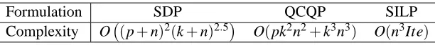
Formulation SDP QCQP SILP Complexity O (p+n)2_(k+n)2.5

O(pk2n2+k3n3) O(n3Ite)

Table 1: Time complexity of the proposed multi-class RKDA kernel learning formulations: p is the number of candidate kernels, n is the number of training samples, k is the number of classes, and Ite is the number of iterations in SILP.

Proof The proof follows the same procedure as in Theorem 2.3 by starting from Equation (36) and changing the definition of Si(β)from Equation (18) to Equation (38).

Note that the only difference between formulations in Theorem 2.3 and Theorem 3.3 lies in the definitions of Si(β). To find theβj, for j=1,···,k,that maximize the constraint violation in the

multi-class case, we need to solve the following k systems of linear equations:

1 2I+

1 2λ

p

∑

i=1

θi_G˜_i !

βj=hj, for j=1,···,k.

Note that the coefficient matrix is the same for all of the k linear systems. Thus the LU decomposi-tion (Golub and Van Loan, 1996) needs to be computed only once, and only the forward/backward substitution needs to be performed k times to obtain the solutions.

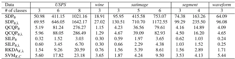
3.4 Time Complexity Analysis

In this subsection, we analyze the time complexity of the proposed formulations in the multi-class case. By following similar analysis in the binary-class case, we can show that the proposed (approx-imate) SDP and QCQP formulations have worse-case time complexity of O (p+n)2_(k+n)2.5

and O(pk2n2+k3n3), respectively. For the SILP formulation in the multi-class case, the k linear sys-tems involved in each iterative step share the same coefficient matrix, and they can be solved in O(n3_{)time. Thus, the overall complexity is still O(n}3_{Ite)where Ite is the number of iterations. The} complexity of multi-class RKDA kernel learning formulations is summarized in Table 1.

4. Joint Kernel and Regularization Parameter Learning

The formulations presented in the last two sections focus on the estimation of the kernel matrix only, while the regularization parameter λis pre-specified. In some cases, the performance of RKDA algorithm depends critically on the value ofλ. In this section, we show that all the formulations proposed in this paper can be reformulated equivalently, and this new formulation leads naturally to the estimation of the regularization parameterλin a joint framework. The detailed derivations in this section are similar to those presented in Sections 2 and 3.

4.1 Joint Learning for Binary-class Problems

framework. In particular, all the formulations (SDP, QCQP, and SILP) for the binary-class RKDA kernel learning problems, presented in Theorems 2.1–2.3, can be recast to optimize the regulariza-tion parameter simultaneously. The next three subsecregulariza-tions provide details of these reformularegulariza-tions.

4.1.1 SDP FORMULATION

For the estimation of regularization parameter, we consider a slightly modified version of the regu-larized least squares formulation, which is equivalent to the standard formulation in Equation (12). The modified version minimizes the following objective function:

F7(w,K,τ) =τ||(φK(X)P)Tw−a||2+||w||2, (39) whereτ=1/λ. We will first consider the case whenτis fixed. We will then extend to the general case whenτis optimized jointly.

The optimal w∗that minimizes the objective function in Equation (39) for a fixed K and a fixed

τis given by

w∗ =

1

τI+φK(X)PφK(X)T

−1

φK(X)Pa

= τφK(X) I₋P

1

τI+PGP

−1 PG

! a.

The optimal value of the objective function in Equation (39) is given by

F₇∗(K,τ) =aT

1

τI+G˜

−1

a, (40)

where ˜G=PGP.

We can observe from Equation (40) that the identity matrix appears in exactly the same form as other kernel matrices. We can thus treat the regularization parameter as one of the coefficients for the kernel matrix and optimize them simultaneously. This leads to the following formulation:

min_t,θ˜ t subject to

∑p

i=0θi˜ G˜i a

aT t

0,

˜

θ_≥0,

p

∑

i=0 ˜

θitrace(G˜i) =1, (41)

where ˜θ= [θ0,θ1,···,θp]T,θ0=1_τ =λ, and ˜G0=I. 4.1.2 QCQP FORMULATION

in Theorem 2.2, the optimization problem in Equation (15) can be expressed as

min

θ:θ≥0,θT_r=1maxβ

(

−1₄βT 1_τI+ p

∑

i=1

θi_G˜_i !

β+βTa )

= max

β _θ˜_{: ˜θ≥}min_0,θ˜T_r=1

( −1₄βT

p

∑

i=0 ˜

θi_G˜_i !

β+βTa )

, (42)

whereθ0= 1_τ, and ˜G0=I. This can be formulated to optimize the regularization parameter as one of the coefficients for the kernel matrix as follows:

max

β,t β

T_a

−1₄t

subject to t_≥ 1 ri

βT_G˜iβ,i=0,

···,p. (43)

This problem is a quadratically constrained linear program.

4.1.3 SILP FORMULATION

The SILP formulation proposed in Theorem 2.3 for the binary-class problem can also be reformu-lated to optimize λjointly. It follows from Equation (42) that this joint learning problem can be formulated as follows:

max ˜

θ,γ γ

(44)

subject to θ˜_≥0, ˜

θT_r=1, p

∑

i=0

θiSi(β)≥γ, for allβ,

where Si(β)is defined as

Si(β) =

1 4β

T_{G˜iβ−riβ}T_{a, for i=0,···,p,}

r= (r0,···,rp)T, ri=trace(G˜i), ˜θ= [θ0,θ1,···,θp]T,θ0=1_τ =λ, and ˜G0=I. 4.2 Joint Learning for Multi-class Problems

4.2.1 SDP FORMULATION

In order to incorporateλin the optimization problem, we modify the objective function in Equation (26) as follows:

F8(W,K,τ) =

k

∑

i=1

(wT_i φK(X)hi)2 wT

i (τΣK+I)wi

.

By following the same derivation in Lemma 3.1 and noticing the relationship with the binary-class case, we derive the following SDP formulation for the multi-class RKDA kernel learning problem:

min

t1,···,tk,θ˜

k

∑

j=1 tj

subject to 

     

∑p

i=0θi˜ G˜i h1 h2 ··· hk

hT₁ t1 0 ··· 0

hT₂ 0 t2 ··· 0

..

. ... ... ... ...

hT_k 0 0 ··· tk



     

0,

˜

θ≥0, ˜

θT_{r=1, (45)}

where ˜θ= [θ0,θ1,···,θp]T,θ0=1_τ =λ, and ˜G0=I. 4.2.2 QCQP FORMULATION

Similar to the binary-class case, we modify the least square problem in Equation (33) as follows:

F9(W,K,τ) =

k

∑

i=1

τ_||(φK(X)P)Twi−hi||2+||wi||2

,

whereτ=1/λ. By following the same derivation as in Theorem 3.2, we obtain the following joint optimization problem:

max

β1,···,βk,t k

∑

j=1

βT jhj−

1 4t

subject to t_≥ 1 ri

k

∑

j=1

βT

jG˜iβj,i=0,···,p. (46)

4.2.3 SILP FORMULATION

Similar to the reformulation in the binary-class case, the SILP formulation for multi-class problems can also be formulated to optimizeλsimultaneously as follows:

max ˜

θ,γ γ (47)

subject to θ˜_≥0, ˜

θT_r=1, p

∑

i=0

θiSi(β)_≥γ, for allβ,

where

Si(β) = k

∑

j=1

1 4β

T

jG˜iβj−riβTjhj

, for i=0,_···,p,

r= (r0,_···,rp)T_{, r}

i=trace(G˜i), ˜θ= [θ0,θ1,···,θp]T,θ0=1_τ =λ, and ˜G0=I.

The reformulations to optimize λsimultaneously proposed in this section are motivated from Lanckriet et al. (2004b) and De Bie et al. (2003). As has been show in Lanckriet et al. (2004b), this joint optimization ofλ works well in most cases in comparison with the simple approach of pre-specifyingλ, but improved performance is not guaranteed.

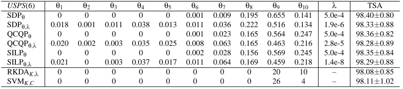
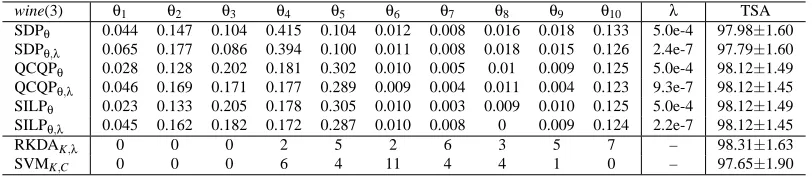
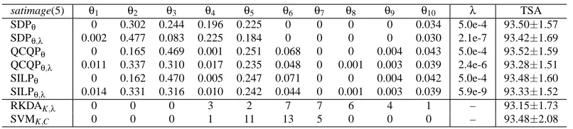
5. Experimental Study

We conduct extensive experiments in this section to compare various aspects of relevant algorithms. The first part of the experiments focuses on combining kernel matrices derived from a single source of data. We demonstrate the effectiveness of the proposed MKL formulations for heterogeneous data integration in the second part of the experiments. The SDP formulations in Equations (8), (32), (41), and (45) are solved using the optimization package SeDuMi (Sturm, 1999). The QCQP formu-lations in Equations (13), (34), (43), and (46) are solved using the MOSEK package (Andersen and Andersen, 2000). The linear programs involved in the SILP formulations in Equations (16), (37), (44), and (47) are solved using the MATLAB1build-in function linprog. The tolerance parameterε, defined in Equation (22), is set to 5_×10−4_{. The source codes of the proposed formulations for the} experiments are available online.2

We first evaluate the proposed formulations for binary-class problems in Section 5.1. The ex-perimental results and analysis for the multi-class formulations are presented in Section 5.2. We demonstrate the effectiveness of the proposed formulations for heterogeneous data integration in Section 5.3. In Section 5.4, we analyze the relationship between RKDA and SVM, and Section 5.5 studies the effect of regularization parameter on classification performance.

5.1 Experiments on Binary-class Problems

In the binary-class case, we compare our formulations with the 1-norm soft margin SVM, 2-norm soft margin SVM with and without the regularization parameter C optimized jointly as proposed in

1. The URL ishttp://www.mathworks.com.

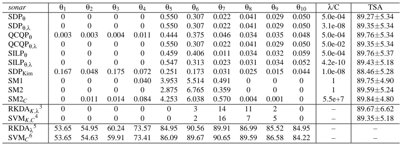
sonar θ1 θ2 θ3 θ4 θ5 θ6 θ7 θ8 θ9 θ10 λ/C TSA SDP_θ 0 0 0 0 0.550 0.307 0.022 0.041 0.029 0.050 5.0e-04 89.27_±5.34 SDPθ,λ 0 0 0 0 0.550 0.307 0.022 0.041 0.029 0.050 3.1e-08 89.35±5.34 QCQP_θ 0.003 0.003 0.004 0.011 0.444 0.375 0.046 0.034 0.035 0.048 5.0e-04 89.76±5.34 QCQP_θ,λ 0 0 0 0 0.550 0.307 0.022 0.041 0.029 0.050 5.0e-02 89.35±5.34 SILPθ 0 0 0 0 0.459 0.406 0.011 0.034 0.032 0.059 5.0e-04 89.76±5.37 SILP_θ,λ 0 0 0 0 0.547 0.313 0.023 0.031 0.034 0.052 4.2e-10 89.43_±5.18 SDPKim 0.167 0.048 0.175 0.072 0.251 0.173 0.031 0.025 0.015 0.044 1.0e-08 88.46±5.28

SM1 0 0 0 0.040 3.953 5.514 0.491 0 0 0 1 89.75±4.90

SM2 0 0 0 0 2.875 6.765 0.359 0 0 0 1 89.59±5.24

SM2C 0 0.011 0.014 0.084 4.253 6.038 0.570 0.004 0.001 0 5.5e+7 89.84±4.80

RKDAK,λ3 0 0 0 0 0 3 14 11 2 0 – 89.67±6.62

SVMK,C4 0 0 0 0 0 2 16 7 5 0 – 89.35±5.18

RKDAλ5 53.65 54.95 60.24 73.57 84.95 90.56 89.91 86.99 85.52 84.95 – – SVMC6 53.65 54.63 59.91 73.41 86.09 89.67 90.65 89.59 86.58 84.22 – –

Table 2: Comparison of twelve methods on the sonar data set. The twelve methods, listed from top to bottom are: SDP formulation with λ fixed as proposed in Theorem 2.1, SDP formulation with λ optimized jointly as proposed in Equation (41), QCQP formulation withλfixed as proposed in Theorem 2.2, QCQP formulation withλoptimized jointly as proposed in Equation (43), SILP formulation with λfixed as proposed in Theorem 2.3, SILP formulation with λ optimized jointly as proposed in Equation (44), SDP formu-lation proposed in Kim et al. (2006), 1-norm soft margin SVM, 2-norm soft margin SVM without and with C optimized as proposed in Lanckriet et al. (2004b), RKDA and SVM with the kernels and regularization parameters selected by double cross-validation. Generally, subscripts of names in the first column are used to denote quantities that are optimized. The ten pre-specified kernels are all RBF kernels and the σ values used are 0.10,0.22,0.46,1.00,2.15,4.46,10.00,21.54,46.42,100.00,as in Kim et al. (2006). The table is partitioned into three sections row-wise. In the first section, the columns headed with θi are the coefficients learned from the corresponding methods. The coef-ficients for the proposed six formulations are normalized to sum to one while those for other compared approaches are reported as obtained from their formulations. The column headed withλ/C provides the values of the regularization parameters, whether fixed or learned, and the test set accuracies and standard deviations are given in the last column. The second section includes RKDA and SVM with kernel and regularization parameter chosen by double cross-validation. We also report the number of times that a particular kernel is selected by cross-validation. The third section shows the accuracies of RKDA and SVM when the kernel is fixed and the regularization parameters chosen by cross-validation. Dashes are used to denote non-applicable items.

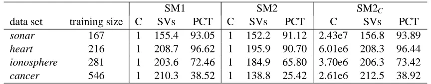
Lanckriet et al. (2004b), and the SDP formulation proposed in Kim et al. (2006). Also, we use double cross-validation to choose kernels and regularization parameters for SVM and RKDA. The 1-norm SVM classifier used is the LIBSVM package (Chang and Lin, 2001) and the 2-norm SVM code was obtained by adapting Anton Schwaighofer’s implementation.7

Four data sets are used in the binary-class case. The sonar, ionosphere, and cancer data were retrieved from the UCI Machine Learning Repository (Newman et al., 1998). The heart data were

3. The number of times that a kernel is chosen by doubly cross-validated RKDA over 30 randomizations. 4. The number of times that a kernel is chosen by doubly cross-validated SVM over 30 randomizations.